A Minimum Route for Machine Tool Travel
M.A. Rahbary1
This paper presents an algorithmic approach to solving the problem of excessive travel in C.N.C. machine tools, by introducing an ecient method to compute the shortest path between given sets of points (origin and destination) in anR2(x;y) plane. When a work piece is located (as an obstacle) between sets of points, it is proved that the optimum path between these points would be formed by sequences of connected straight line segments whose intermediate end points are vertices of an appropriate polygonal (closed control barrier). The case of one origin, one destination and a set of barriers is considered. This method is computationally ecient.
INTRODUCTION
The study of numerically controlled machine tool sys-tems indicates that there are many elements which play a major role in increasing cycle times. Since manu-facturing eciency is directly inuenced by machining cycle time, the attention given to its reduction has always been great. One of the main elements, which contributes to the problem of higher cycle time, is the inecient travel of cutting tools.
The central objective of this paper, therefore, is the development and initial implementation of an algorithm for planning a suitable path for cutting tools to travel, which results in a reduction of the cycle time for manufacturing a part on a machine tool. The problem of nding an optimum path between given points in the presence of barriers has received some attention in the past, but there have been very few publications of the ndings. Some of these algorithms are proven to be computationally inecient or are dicult to implement for a particular case.
Of these published algorithms, the oldest is in [1] where the authors studied the problem of displacement of an autonomous vehicle on Mars and the latest is in [2] where the author investigated strategies of cutter path optimization. Shkel and Lumelsky [3] investigated the problems of nding the shortest smooth path between two points in the plane for robotics applications. Vaccaro [4] discussed the problem of routing an urban vehicle. The routing was considered independently, but the barriers were also represented by line segments.
Wang Dahl, Pollock and Woodward [5]
investi-1. Department of Manufacturing Engineering, Tabriz Uni-versity, Tabriz, I.R. Iran.
gated the shortest pipeline layout between two points on a ship (with polygon barriers). Larson and Li [6] allowed the polygons to be convex or non-convex, but only the rectilinear (Li) norm was considered.
Viegas [7] developed an O(n3) algorithm for the gen-eration of the shortest-paths network in the context of evaluating pedestrian displacements from home to public facilities in towns, using Euclidean distance.
ASSUMPTIONS AND PROBLEM
FORMULATION
It is desired to route a tool tip from a specied start position to another position within a two-dimensional work space, avoiding interferences with barriers placed in between the positions. If one or more paths exist, as usually is the case, the shortest route must be found.
The following assumptions are made:
1. Only the case of a single origin and destination in the presence of a single barrier and in the planeR2 is considered. However, the technique is extendable to more than one barrier and sets of origins and destinations. It could also be dened to work in a three-dimensional work space;
2. All boundaries (of the space and of the barrier) are composed of straight-line segments;
3. It is required to nd the shortest distance between any origin and destination, such that these paths do not cross any barrier;
4. Barriers are convex or non-convex closed polygons; 5. No points of origin or destination are located inside
or on the barriers;
METHOD
The principal problem of nding an optimum path be-tween a set of points (origin and destination) is broken down into a sequence of minor or local problems, which can be dealt with one at a time.
A set of origins,O=fo 1
g, and destinations,D= fd
1
g, in the plane R
2, and a set of barriers to travel,
B=fb 1
g, are introduced. Before proceeding with any calculation of an optimum path for any point, it is, rst, necessary to reduce the problem to a network or matrix representation. To do this, it is required to dene control lines drawn parallel to the boundaries of the barrier in question, in order to dene the control barrier. Control points on the control barrier are the only dened points through which an optimum path could pass.
Geometrically, a `control point' is dened to be the intersection of two straight lines that are adjacent members of the set of straight lines forming the super scribing polygon (control polygon or barrier) around a piece of equipment. The sides of this polygon are a prescribed perpendicular clearance distance (say d) from their respective parallel equipment boundaries.
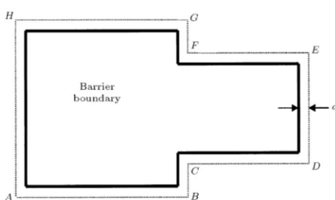
Figure 1 illustrates the generation of such control pointsA,B,C,D,E,F,GandH for a polygon.
The following notation is used: The barrier (dened by control points) denoted `b' (control bar-rier), is dened by the list of its vertices, Vb =
fV
0;V1;V2;V3;
Vmg, where (m + 1) denotes the number of vertices of the barrier. This list corresponds to successive vertices from one end of the barrier to the other.
PROPERTIES OF SHORTEST PATHS
NETWORK
A few concepts and some theories are rst introduced: 1. A point is said to be visible [8] from a point if and only if, the straight line segment joining these two points crosses no barrier. To solve the problem of inter-visibility as a practical matter,
Figure1. Control points for a closed polygon.
it is important to describe a way to determine the visibility of one point from another. Here, a straightforward technique follows. Consider the situation in Figure 2. The segment [P1 P2] joining pointsP1andP2, is a boundary or a control line. It can be said that the line joiningP1andP2 consists of all points (x;y), such that:
x=xp1+ (1 )xp2;
y=yp1+ (1 )yp2; (1)
where: 01:
Similarly, the line joining i and j consists of all points (x;y), such that:
x=xi+ (1 )xj;
y=yi+ (1 )yj; (2)
where: 01:
Solving Equations 1 and 2 simultaneously forand
gives:
= (xp2 xj)(yp1 yp2) (yp2 yj)(xp1 xp2) (xi xj)(yp1 yp2) (yi yj)(xp1 xp2)
; = (xp2 xj)(yi yj) (yp2 yj)(xi xj)
(xi xj)(yp1 yp2) (yi yj)(xp1 xp2)
:
Foriandj not to be visible, both conditions: 0< <1 and 0< <1 must be true.
For all other values of and , i and j are visible. If:
(xi xj)(yp
1 yp2) (yi yj) (xp
1 xp2)=0; the lines are parallel, there is no intersection andi
andj are visible.
Figure3. Locally and globally supporting lines of a barrier.
2. The lineLi (see Figure 3) is locally supporting the
barrier,b(closed polygon), because:
(i) Li contains one vertex at least ofb(P1); (ii) All the points belonging to the intersection
of an arbitrarily small circle, C, of radius \r" centered at point Pj, lie on one of the
two closed half-planes dened by Li, subject
to the direction in which the shortest path is considered. If the negative ( ) direction is considered, then, the intersection points should lie on, or to, the left of the half-plane, or else to the right of the half-plane.
Li is a locally supporting line of the barrier at
P1. The intersection pointsx1 and x2 are entirely located to one side of the lineLi, (left half-plane);
3. The lineGs1is globally supporting barrierb(closed polygon), because:
(i) The line Gs1 contains one vertex at least of barrierb (P3);
(ii) The lineGs1satises the Case (2) and, there-fore, locally supports the barrier,b, atP3; (iii) All the vertices of the barrier, b, lie entirely
on, or to one side of the line. This condition is also subject to the direction of scanning.
Gs1is a globally supporting line of the barrier,
b, at P3 and also a locally supporting line at P3 (scanning in a ( ) direction), where the vertices (P0, P1, P2, P3, P4, P5, P6), lie entirely to one of two sides dened by the segment Gs1. The line, Gs2, is also globally supporting the barrier,
b, at P0 (scanning in a ( ) direction). From the situation discussed above, it can be said that in anyx=y plane (R2) and in the presence of a single point and a barrier, there can only be two globally
supporting lines to that barrier (Gs1, Gs2), as in Figure 3.
Theorem
When distances are measured with Euclidean distance, any optimum path is composed of connected straight line segments, where;
(a) xo is an origin;
(b) xd is a destination;
(c) vj withj = 0;1;2;;k is a vertex of the barrier
b(j), such that the shortest path connectingxoand
xd intersects the barrier at its vertices and each
intersection point is the second point of the line segment, which, in turn, is a supporting line of the barrier at that intersection point.
Proof
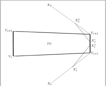
As a shortest path consists of a straight line between two mutually visible points, consider three consecutive line segments [xo;vj+1], [vj+1;vj+2] and [vj+2;xd], as illustrated in Figure 4, on the shortest feasible path. The path is assumed to be nonlinear, otherwise vj+1 andvj+2would be irrelevant and may be deleted from the path.
Now, consider points x0 1, x
00 1, x
0
2 and x 00 2 at an arbitrarily small distance, (r > 0), from vj+1 and
vj+2, respectively. Consider another path, which is composed of [x0;x
0 1], [x
0 1;x
00 1], [x
00 1;x
0 2], [x
0 2;x
00 2] and [x00
2;xd], which is shorter than the path composed, [xo;vj+1], [vj+1;vj+2] and [vj+2;xd]. This is true because of the triangle inequality. So, the shortest path, which consists of segments of [xo;x0
1], [x 0 1;x
00 1], [x00
1;x 0 2], [x
0 2;x
00
2] and [x 00
2;xd], cannot be a feasible one and must be deleted. The earlier path, withx0
1located on the segment [xo;vj+1] and x
00 1 on [vj
+1;vj+2], is
Figure 4. Shortest path and barrierbfor the proof of the theorem.
entirely positioned on one half dened by the line [xo;vj+1] and the vertices of the barrier, b, are also located on that half.
So, one can say that the line segment [xo;vj+1] is a globally supporting line of barrier b at point
Vj+1. With the same principle, [xd;vj+2] is a globally supporting line of the barrierbat pointvj+2. One can also say that the only feasible shortest path connecting
x0 to xd is a path which consists of the straight line segments [xo;vj+1], [vj+1;vj+2] and [vj+2;xd].
GENERAL SOLUTION
Initialization
Select the total of Nb control points and let (Xib;Yib)
be the coordinate of theith control point where;
ib= 1;2;3;;Nb:
By convention, ob is assigned as the origin and
db as the destination. Points ob and db are said to
be visible if a straight line joining them does not intersect the boundary of the control lines (visibility test theorem).
If ob and db are visible, then, one can dene
the path which is composed of a straight line, [ob;db],
and the problem is solved. Otherwise, compute the distance,rib, fromobanddb to every point (Pib) ofXb,
where Xb is associated with the set of vertices of the
barrier:
Xb=fP
1;P2;P3;
;Pnbg;
Rob=fr
1b;r2b;r3b;
;rmbg;
Rdb=fr
1b;r2b;r3b;
;rmbg:
The set, Rob, is associated with the set of distances
which are related toob and vertices inXb and the set,
Rdb, is related to dband vertices in Xb. Let ro be the
minimum distance associated withob and rd with db.
Now, nd the corresponding vertices of these minimum members from setXband let them be dened asP0and
Pd.
Scanning Phase
Now, precede scanning in clockwise and anti-clockwise directions forob anddb, respectively, starting from the
barrier vertex corresponding to the minimum distances (ro;rd) and their respective points (Po andPd).
Com-pute the globally supporting points (see setsGob and
Gdb). In either direction, for bothob anddb. Let:
Gob=fPig;
and:
Gdb=fPig:
If setsGobandGdbshared a common member (letPibe
the common member) in their sets, then compute that point. Connectob toPi anddb, whereob anddb must
be inter-visible viaPi. The set should be computed as:
Sb=fob;Pi;dbg:
If the condition mentioned for the sets was not satised, proceed with scanning.
The scanning should start in both directions (clockwise and anticlockwise), from the rst globally dened point and ending at the destination point,db.
Any segment (Pj;Pk), wherePjandPkrepresent
the start and end points of a globally dened line, may be handled by the following procedures (now the tests are being carried out on the segments of the barrier itself,Pj andPk are the vertices of the barrier):
1. Start, for example, with Pj in an anticlockwise
direction. Take the segment (Pj;Pj+1) and carry out the globally supporting lines test. IfPj+1passes the test, insert it in the list of live vertices (setS1b); 2. Go to the next vertex (say in the anticlockwise direction, Pj+1) and carry out Step 1. Continue the procedure until one of the segment's end points is also a member of the set, Gdb. Now, complete
S1b by computing the last point. The set, S1b, represents the rst feasible path;
3. Continue the steps above in a clockwise direction, starting with Pj. Complete S2b by computing all the barrier's vertices which pass the test;
4. S1b and S2b hold two dierent sets of paths which connectob todb. Using a Euclidean distance
calcu-lation, select the set which produces the optimum path.
The path with the minimum value is the shortest feasible path which connects ob to db and satises the
conditions for an optimum path.
EXAMPLE OF HOW THE ALGORITHM
WORKS
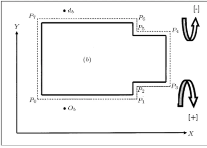
Consider now a small example, using Euclidean dis-tance, in Figure 5. Select the the control points as starting with barrier vertices (0-7), destination db
and origin ob. Register the Cartesian coordinates of
these points, as presented in Table 1. To check the visibility of ob and db an algorithm is executed for
visibility presented earlier. If these points are inter-visible, terminate the process, or else, resume with the following procedures:
Figure5. Control geometry for the example.
Table1. Coordinate for the points of the example.
Point
No.
X Y Barrier vertices P0 4 6P1 9 6
P2 9 7
P3 11 7
P4 11 9
P5 9 9
P6 9 10
P7 4 10
Origin - 6 5
Destination - 6 11
1. Compute the Euclidean distance ofob anddb from
all the vertices of barrierb (Table 2);
2. Select the vertex corresponding to the smallest element in both lists (P0 andP7, respectively); 3. Scan forobin an anticlockwise ( ) direction,
start-ing with the smallest element in Table 2, as found in the above step (P0). Note that the condition for globally denable lines for a ( ) direction is not the same as for a (+) direction, (see the denition of globally dened lines in the previous section); 4. Segment [ob P0] does not satisfy the conditions for
a globally supporting line and, therefore, is deleted. [ob P0] satises the conditions and, therefore, the segment [ob P1] should be registered. Proceed scanning in the opposite direction (+). The line, [ob P1], satises the condition and, so, should be computed. The completed set should be computed as:
Gob =fP 1;P0
g:
5. Resume the scanning operation, starting with point
d and carry out Steps 2 to 4. The completed set should be computed as:
Gdb=fP 7;P6
g:
6. Sets Gob and Gdb do not have a common element
and scanning should be resumed. Move to pointP1, (P1"Gob) and scan in the ( ) direction, starting with the segment [P1;P2]. [P1;P2] is a segment connecting two vertices of the barrier and is subject to globally supporting lines denition tests: a) At [P1;P2]; 7:[P1;P2] does not satisfy the
con-dition for a globally supporting line;
b) At [P2;P3]; 8:[P2;P3] supports the conditions for a globally supporting line and should be computed;
c) At [P3;P4]; 9:[P3;P4] satises the condition for a globally supporting line atP4;
d) At [P4;P5]; 10:[P4;P5] does not satisfy the conditions for a globally supporting line; e) At [P5;P6]; 11:[P5;P6] satises the conditions
for a globally supporting line at P6;
f) At [P6]; 12:P6 is a supporting vertex, which is also a member ofGdb. So,P4 anddb are visible via the vertex P6. So, compute the set S1 = fob;P
1;P3;P4;P6;db
g, which comprises the line segments [ob;P1], [P1;P3], [P3;P4], [P4;P6] and [P6;db].
The sweep is terminated and the segments which complete the path are registered. The sweep from
ob towards db could be achieved on either side of
the barrier, b (clockwise ( ) or anticlockwise (+) directions). Now, proceed in the opposite direction, which, in this case, is the clockwise (+) direction and repeat procedures 2-13. The result of this sweep can be shown as the setS2=
fob;Po;dbgand the line segments [ob;Po][Po;P7] and [P7;db].
SetS1andS2represent the two dierent patterns which dene the shortest path to connect ob to db
Table 2. The distances for the example.
Points No. Distance
(Origin)
(Destination)
Distance
P0 2.23 5.38
P1 3.16 5.38
P2 3.60 5.00
P3 5.38 6.40
P4 6.40 5.38
P5 5.00 3.60
P6 5.83 3.16
without crossing the barrier in either direction. One of these sets (S1 andS2) contains the optimum route. By comparing the two,S2 with the segments [ob;Po], [Po;P7] and [P7;db], can be seen to be the optimum.
IMPLEMENTATION IN
MANUFACTURING
Computer Numerical Control (CNC) machine tools are amongst the most important and most complex machines in the manufacturing world. The increasing complexity of engineering components requires an in-crease in safety, productivity, system reliability, greater operator satisfaction and a signicant reduction in machine down-time in the implementation of these machines. The introduction of the algorithms (shortest path and visibility) in this paper is aimed at producing a method which could be implemented in manufactur-ing to reduce the machinmanufactur-ing cycle time by increasmanufactur-ing the speed and accuracy of the operations.
Although these algorithms have many implemen-tations, three stages have been introduced, where they can signicantly improve speed and accuracy in CNC machine tool operations.
It must be emphasized that such techniques have not been used in any of the modern CAD/CAM systems, due to complexity in the C.N.C. operating environment. The method introduced makes the implementation of such an approach computationally possible, as shown in this paper.
These algorithms could be used in nding a suitable path between any two spatial points in a continuously changing environment. This changing en-vironment could be due to alteration in a component's geometry or in the positions of any moveable part of the machine tool. This concept is best described in Figure 6.
Figure6. Non-optimized and optimized tool path between pointsAandB.
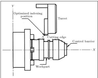
The algorithms could also be used in optimising the indexing position during the cutting operations. The position control for indexing operations would be based on safety and speed. Figures 7a and 7b describe the concept.
The position control of the tool tip could also be achieved by implementing the algorithms for this purpose. The position of the tool tip is continuously monitored in reference to the next position and is com-puted according to the safety margin created around the work-piece. This concept is also described in Figures 8a and 8b.
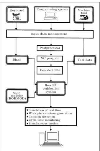
Figure 9 shows how the complete system can be implemented and used as an extension of the existing CAD/CAM systems.
Figure 9 represents an optimization system which has been created using the technique introduced in this paper. It is aimed to be used in conjunction with a
Figure7a. Non-optimized indexing position for upper turret before moving to pointA.
Figure7b. Optimized indexing position for upper turret before moving to point A.
Figure8a. Non-optimized position of tool tip prior to a cutting operation.
Figure8b. Optimized position of tool tip prior to a cutting operation.
modern CAD/CAM system and as a separate module. This system oers functions such as:
1. Simulation of N.C. operations using an N.C. pro-gram received from a CAM system;
2. Automated work piece contour generation and up-date using the technique introduced in this paper; 3. Automated collision detection and avoidance; 4. Cycle time reduction, using the tool tip travel
optimization techniques introduced.
CONCLUSION
The algorithms described have been successfully pro-grammed in `C++'. The method is based on nding vertices corresponding to the control barrier, which would be the only feasible vertices able to form the segments of the optimum path. The algorithm is par-ticularly designed to suit a CNC dynamic environment,
Figure 9. Data ow in the dynamic verication system implementing the algorithm.
but, at the same time, its generality has been preserved by presentation as an independent algorithm.
The advantage of this algorithm is that it can be easily developed, computerized and implemented for practical purposes. Also, the system supports the case of one barrier and one set of origins and destinations in the plane, R2, as is the case in any machining operation.
It must be noted that the current and modern CAD/CAM systems have never implemented similar techniques, due to the complex dynamic environment presented by C.N.C. operations.
REFERENCES
1. Kirk, D. and Lim, L. \A dual-mode routing algorithm for an autonomous roving vehicle",IEEE Transactions on Aerospace and Electronic Systems, 6, pp 290-294 (1970).
2. Toh, C.K. \Cutter path strategies in high speed ma-chining of hardened steel",Materials&Design, Article in Press (2004).
3. Shkel, A.M. and Lumelsky, V. \Robotics and au-tonomous systems classication of the Dubins set 1",
Robotics and Autonomous Systems,34(4), pp 179-202 (31 March 2001).
4. Vaccaro, H. \Alternative techniques for modeling travel distance", MA. Thesis in Civil Engineering, Massachusetts Institute of Technology, USA (1974). 5. Wang Dahl, G., Pollock, S. and Woodward, J.
\Mini-mum trajectory pipe , J. \Mini\Mini-mum trajectory pipe routing", Journal of Ship Research, 18, pp 46-49 (1994).
6. Larson, R. and Li, G. \Facility locations with the Man-hattan metric", The Presence of Barriers to Travel. Operations Research,31, pp 652-669 (1983).
7. Viegas, J. \Capacity expansion in public facility net-works", Doctoral Thesis in Civil Engineering, Institute Superior Tecnico, Lisbon, Portugal (1984).
8. Goldman, A.J. \A theorem on convex programming", Paper presented at MAA Meeting, Annapolis, MD, USA (1963).