Sharif University of Technology
Scientia IranicaTransactions A: Civil Engineering www.scientiairanica.com
A comparison of ve dierent models in predicting the
shear stress distribution in straight compound channels
Z. Sheikh Khozani
and H. Bonakdari
Department of Civil Engineering, Razi University, Kermanshah, Iran.
Received 7 April 2015; received in revised form 9 September 2015; accepted 5 October 2015
KEYWORDS Compound channel; Floodplain;
Main channel; Shear stress distribution; Traditional models; Wetted perimeter.
Abstract. The ability of ve dierent methods to estimate the shear stress distribution in compound channels is investigated. Methods proposed by Yang and Lim (YLM), Khodasheans and Paquier (KPM), Sterling and Knight (SKM), Zarrati et al. (ZAM), and Bonakdari et al. (BAM) are compared with experimental data. YLM and KPM did not provide reliable results as they produced higher Mean Absolute Percentage of Error (MAPE) values of 25-55%. SKM performed adequately in predicting the pattern of shear stress distribution on the main channel bed, but on a oodplain bed; it predicted a constant value over the entire wetted perimeter. The SKM method outperformed YLM and KPM with 2 to 20% MAPE. The ZAM and BAM methods produced the best results for shear stress distribution in compound channels with average MAPE of 2.67 and 5.66% MAPE , respectively. Although ZAM showed more accurate results than BAM, however, BAM required solving much fewer equations than ZAM and presented more accurate results than other geometric methods. Among all models, BAM is proposed as a simple and accurate model for predicting the shear stress distribution in compound channels.
© 2016 Sharif University of Technology. All rights reserved.
1. Introduction
Most of the time, natural river cross sections are found in compound channels, and studying these sections is of specic signicance in river engineering and ood risk management. Important concerns in river hydraulics include sedimentation and the transport of solids within these types of cross sections. Shear stress is one of the important problems in sediment transport processes. In many cases, boundary shear stress on the channel wall is predicted in the form of an average value shear stress on the channel wall and bed [1-3]. For many years, a large number of experimental investigations have been carried out in open channels. Studies have shown that it is dicult to
*. Corresponding author. Fax: +98 3137717221 E-mail addresses: [email protected] (Z. Sheikh Khozani); [email protected] (H. Bonakdari)
determine the boundary shear stress distribution in an open channel [4-9]. To overcome this diculty, empir-ical, analytempir-ical, and simplied computational methods have been conducted by several researchers [10-21]. Still, even with sophisticated turbulence models, it is challenging to accurately calculate local shear stress values.
Because channel geometry has an important role in variations of boundary shear stress, several theoret-ical studies have been developed based this concept. Khodashenas and Paquier [11] employed a geometri-cal method to compute the shear stress distribution by measuring the depth perpendicular to the wall (KPM). In this method, the impact of secondary ow structures and the transfer of momentum between the main channel and its oodplains are neglected. The Shannon entropy concept has been applied by several researchers to predict the shear stress distribution in open channels [12,21-23]. Sterling and Knight [12]
developed a new approach to predict the distribution of boundary shear stress in open channels (SKM) based on Shannon entropy. Although their proposed method has limitations in reecting the hydraulic behaviour of open channels, the results indicated that the method could estimate shear stress distribution reasonably well, but it must be developed for practical applica-tions. Yang and Lim [10,14] suggested the transport of surplus energy over the shortest relative distance towards the wall within steady, uniform, and fully developed turbulent ow. They [15] dened a relative distance as the minimum geometrical distance ratio for the energy dissipation capacity of the boundaries (YLM). Based on this concept, the authors proposed an analytical equation for local and mean boundary shear stress along the wetted perimeter. In their model, the impact of secondary current on shear stress was not taken into account either. The semi-analytical equations proposed by Zarrati et al. [24] were aimed to predict shear stress distribution in simple and com-pound channels (ZAM). These equations were obtained by simplifying a stream-wise vorticity equation and considering secondary Reynolds stresses. The model proposed by Zarrati et al. [24] considered the eect of secondary ows, but contained many equations to estimate shear stress distribution, which is time-consuming and requires high precision. Bonakdari et al. [19] estimated the shear stress distribution in dierent channel cross sections using the Tsallis entropy concept and maximized it with the help of Lagrange coecients (BAM). However, the Tsallis method necessitates solving two explicit equations in order to nd the coecient values.
In this research, the ability of ve dierent meth-ods, namely, KPM, SKM, YLM, ZAM, and BAM in estimating shear stress distribution in compound chan-nels is investigated. The cross section of compound channel is illustrated in Figure 1. All these geometrical models are also compared with each other and the most appropriate model in predicting shear stress is introduced. To verify the results, the laboratorial outcomes obtained by Rajaratnam and Ahmadi [25], Myers and Elsawy [26], and Cokljat and Younis [27] are utilized.
Figure 1. Compound channel transverse section characteristics.
2. Review of methods
Five methods for estimating the shear stress distribu-tion in a compound open channel are compared with each other against experimental data. These methods were selected because they are suciently general to predict the shear stress distribution, and they are simple enough for engineering applications.
2.1. Yang and Lim's Method (YLM)
Yang and Lim [10,14] dened a relative distance as the minimum geometrical distance ratio for the energy dissipation capacity of boundaries. For smooth bound-aries, this relative distance represents the dissipation capacity of a boundary with a viscous length scale as v
u
(where v is the kinematic viscosity and uis the shear
velocity), and for rough boundaries, this characteristic length is scaled according to the roughness height. To accomplish this, boundaries are divided according to the transverse section shape.
For a wide channel (b
h > 2), the intersection of
division lines is located above the free surface, and the shear stress distributions of the bed and wall in compound channels (Figure 1) are written according to El Kadi Abderrezzak [16]:
b(z) = gzS; 0 < z H h; (1)
b(z) = g(H h)S; H h< z
B H h
; (2)
b(z) = g(B z)S;
B H h
< z B; (3)
w(y) = gyS; 0 < y (H h); (4)
b(z1) = ghS; 0 < z1
bfp h
; (5)
b(z1) = g(bfp z1)S;
bfp h
< z1 bfp;(6)
w(y1) = gy1S; 0 < y1 h: (7)
Parameter in the above equations is calculated as: 23+2H
B 2+ 1 = 0; (8) where is the uid density, g is the gravitational acceleration, S is the energy slope, b is the channel width, and h is the water depth. For narrow channels (b
h 2) in which line intersections are below the free
surface and considering the experimental data used in the present study relates to wide channel sections, explaining shear stress equations for narrow channel sections is avoided.
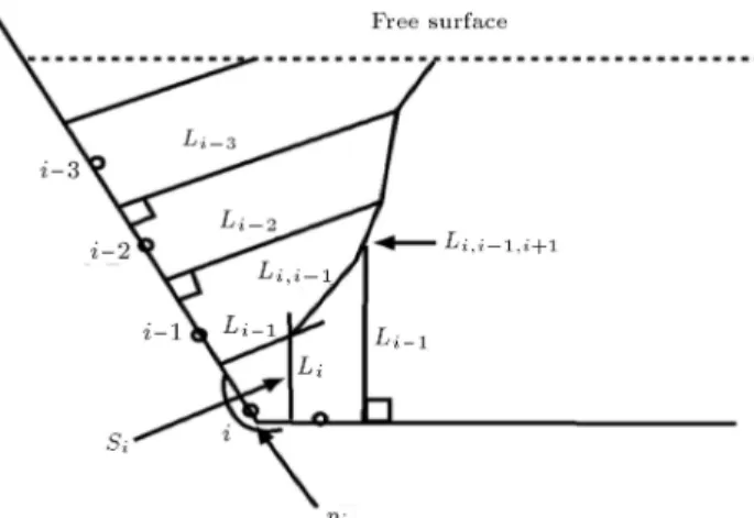
Figure 2. Schematic illustration of the areas determined by KPM.
2.2. Khodashenas and Paquier's Method (KPM)
The normal area method is one of the techniques of estimating shear stress distribution. With this method, the boundary shear stress is estimated from the area between two drowned normal to bed of channel. This method fails when channel walls have a steep slope, because the intersection of normal occurs below the water surface. To solve this problem, Khodashenas and Paquier [11] extended the normal area method and predicted shear stress distribution in an irregular cross section of a channel. The shear stress distribution was calculated as follows:
1. The wetted perimeter is divided into small segments (Figure 2).
2. The mediator of each segment is drawn.
3. When each mediator intersects the normal line, they should merge with each other. The direction of the new line of order 2 created is computed as:
^Li;i 1=12
^Li+ ^Li 1
: (9)
4. When this new line intersects the normal line or other high-order lines, its angle is computed with the weighted mean of the previous line. This pro-cedure continues until the water surface is reached:
^Li;i 1;i+1=13
2^Li;i 1+ ^Li+1
: (10)
5. The area between the nal lines (Si) is calculated
and the shear stress is estimated by:
i= gRhiS; (11)
where Rhi = Si=Pi is the local hydraulic radius, g
is the gravity acceleration, is the water density, and S is the energy slope.
2.3. Sterling and Knight's Method (SKM) Sterling and Knight [12] used the Lagrange coecient to maximize the Shannon entropy and introduce an equation to predict shear stress. Based on this method, the shear stress distribution in a compound channel with the section shown in Figure 1 is predicted as:
b(z) = 1 bmln
1 + (ebmmax(bm) 1)2(z zc)
B
zc< z < B2; (12)
w(y) = 1 wmln
1 + (ewmmax(wm) 1)2(y yc)
H h
yc< y < H h; (13)
b(z1) =1 bfpln
h
1 + (ebfpmax(bfp) 1)i
0 < z1< bfp; (14)
w(y1)=1 wfpln
1+(ewfpmax(wfp) 1)(y1 yc)
h
yc< y1< h; (15)
where w(y) and w(y1) are shear stress at the wall
of the main channel and oodplain, respectively; b(z)
and b(z1) are the shear stress on the bed of the
main channel and oodplain, respectively; max(wfp),
max(bfp), max(wm), and max(bm) are the maximum
shear stress at the wall and bed of the oodplain and main channel; and yc and zc are constant values of
5 mm [12]. Eqs. (12) to (15) are used to predict the shear stress distribution in sub sections of the compound channel shown in Figure 1. In Eqs. (12) to (15), the parameter is calculated as follows:
=
maxemax
emax 1 gRS
1
: (16)
In order to use Eqs. (12) to (15) as well as (16), the mean and maximum shear stress should be calculated earlier. Therefore, the relations presented by Knight et al. [1] are applied as follows:
max(w)
gRS = 0:01%SFw(1 + Pb=Pw); (17) mean(b)
gRS = (1 0:01%SFw)
1 + P 1
b=Pw
; (18) max(w)
gRS = 0:01%SFw
2:0372(Pb=Pw)0:7108; (19)
max(b)
gRS = (1 0:01%SFw)
2:1697(Pb=Pw) 0:3287;
where mean(w)and mean(b)are the mean shear stress at
the wall and bed, respectively; is the uid density; g is gravitational acceleration; R is the hydraulic radius; S is the bed slope; Pband Pware the wetted perimeter
corresponding to the bed and wall of the channel, respectively; max(w) and max(b) are the maximum
shear stress at the wall and bed, respectively; and %SFwis the percentage of shear force carried by walls
and is evaluated as follows:
%SFw= Csfexp ( 3:23 log(Pb=C0Pw+ 1) + 4:6052) ;
(21) where Csf = 1 for Pb=Pw < 4:374, unless Csf =
0:6603(Pb=Pw)0:28125and in subcritical ow C0 = 1:38.
Thereby, for a given channel, depending on the water depth and bed slope, the transverse distribution of shear stress can be estimated.
2.4. Zarrati et al.'s Method (ZAM)
An analytical model was presented by Zarrati et al. [24] to predict the shear stress distribution in channels with rectangular, trapezoidal, and compound cross sections. They derived semi-analytical equations based on a simplied streamwise vorticity equation including secondary Reynolds stresses. In this method, the eect of additional secondary ows is considered, which is due to the shear layer between the main channel and the oodplain. To compute the shear stress on the wetted perimeter of a compound channel, the channel cross section was divided into regions, as shown in Figure 3. Two equations for predicting the shear stress along the bed of a main channel are:
b(z)
mean(bm) = A1 2z B 2z B +2aB1
+ C12zB 0 < z < a; (22)
b(z)
mean(bm) = A2
2z
B + C2; a < z < B
2; (23) where 1 = 0:02, a = H h z0, and z0 =
0:026827 e( 2:812148(h=H 1)) 1b fp.
Figure 3. Geometric parameters of a compound channel [24].
To predict the shear stress on the main channel wall, the following equations are proposed:
w(y)
mean(wm) = A 0 2
y H h y
H h+H h zH h01
+ C0 2Hy h
0 < y < H h z0; (24)
w(y)
mean(wm)=A 0 1
H h y z0
2
+B0 1
H h y z0
+C0
1
H h z0< y < H h: (25)
To calculate the shear stress distribution along a oodplain bed, Eqs. (26) to (28) are used:
b(z1)
mean(bfp) = A1
z1
z0
2
+ B1
z1
z0
+ C1
0 < z1< z0; (26)
b(z1)
mean(bfp)=A2
z1
z0
2
+ B2; z0< z1< bfp a; (27)
b(z1)
mean(bfp) = A3
z1 bfp
bfp
z1 bfp
bfp + 0:02
a bfp
B3z1b bfp fp
bfp a < z1< bfp: (28)
Ultimately, the lateral stress distribution on the ood-plain wall can be calculated with Eqs. (29) and (30):
w(y1)
mean(wfp) = A 0 1
y1
h y1
h +ah1+ C 0 1yh1
0 < y1< a; (29)
w(y1)
mean(wfp) = A 0
2 1
y1
h
1 y1
h +h ah 2
+ C0 2
1 y1
h
;
0 < y1< h: (30)
In these equations, a is the width of the corner region; z0 is the interaction zone width; 2 = 0:02; A1, B1,
C1, A2, B2, C2, A3, B3, and C3, are bed shear
stress distribution coecients; and A0
1, B10, C10, A02,
B0
2 represent wall shear stress distribution. These
coecients can be calculated with some equations mentioned in the Zarrati et al. [24].
2.5. Bonakdari et al.'s method (BAM)
Bonakdari et al. [19] employed the Tsallis entropy to derive the shear stress distribution in dierent channel cross sections based on two simple constraints: (1)
the total probability, and (2) conservation of mass, along with maximizing the entropy function using Lagrange coecients. The parameters of the derived shear stress distribution were determined using these two constraints. They studied the model's accu-racy in circular, circular with at bed, rectangular, and compound cross sections. Only one cross sec-tion of a compound channels was investigated in the study.
Equations were derived for estimating the shear stress distribution in sub-sections of a compound chan-nel as follows:
b(z) = 1 bm
(0
bm)k+B=2bmz
1=k 0
bm
bm
zc z B2; (31)
w(y) = 1 wm
(0
wmk) +Hwmyh
1=k 0
wm
wm
yc y H h: (32)
For a oodplain, the Divided Channel Method (DCM) was employed, and the following equations were ob-tained:
b(z1)=1 bfp
(0
bfp)k+bfp(bbfp z1) fp
1=k 0 bfp
bfp
0 z1 bfp zc; (33)
w(y1) =1 wfp
(0
wfp)k+wfph y
1=k 0 wfp
wfp
yc y1 h: (34)
To compute the Lagrangian coecients and 0,
Eqs. (35) and (36) are used, which are obtained based on two constraints:
[0+
max]k [0]k = kk; (35)
max
[0+ max]k 1 2
1
k + 1[0+ max]k+1
+1 2
1 k + 1[0]
k+1= kk
mean; (36)
where max and mean are the maximum and mean
shear stress values on the wall and bed of the channel. In order to use Eqs. (35) and (36), the average and maximum shear stresses should be previously calcu-lated using the relations presented by Knight et al. [1] and introduced in Eqs. (17) to (21).
3. Shear stress distribution in sub-sections of a compound channel
3.1. Shear stress on a channel wall in a oodplain
With the help of YLM, SKM, KPM, ZAM, and BAM, the shear stress distribution on a compound channel wall in a oodplain is calculated for two dierent heights, h=H = 0:25 and h=H = 0:4, and is shown in Figures 4 and 5. The results are compared with the laboratorial outcomes of Myers and Elsawy [26], where the channel geometry was the same and only the ow depth diered. According to Figures 3 and 4, BAM predicted the most appropriate shear stress distribution results for a oodplain wall compared to other methods. The ZAM method presented smaller error in estimating the shear stress on a oodplain than other methods for h=H = 0:25. ZAM predicted small values for shear stress distribution in the corner region, but estimated more accurate shear stress distribution results for y1
h > 0:2. As seen in Figures 4 and 5, if
the channel geometry did not change, ZAM predicted
Figure 4. Relative shear stress distribution on a oodplain channel wall (h=H = 0:25).
Figure 5. Relative shear stress distribution on a oodplain channel wall (h=H = 0:4).
similar shear stress distribution values. On the other hand, depth variation did not inuence the prediction of shear stress on a oodplain wall using Eqs. (29) and (30).
Moreover, the SKM method predicted results compatible with laboratorial outcomes. The SKM predicted similar values for all wetted perimeters of a oodplain wall, but these values were close to the mean of observed values. The YLM and KPM methods did not produce good prediction results, as on one half of the wall, the results were underestimated; and for the other half, the results were overestimated. The shear stress distribution pattern predicted that using YLM, and KPM forms a sloping line where the shear stress values increase as they approach the water-air interface. It can be deducted that the BAM, SKM, and ZAM methods predicted results close to laboratorial values. All three methods produced reasonable results with percentage of error less than 5%.
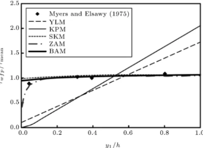
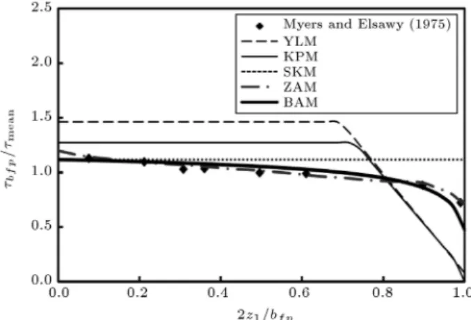
3.2. Shear stress on the oodplain bed
The estimation results for shear stress on the bed of a oodplain are illustrated in Figures 6 and 7. The bed shear stress values are calculated for two dierent heights with ratios of h=H = 0:325 and h=H = 0:5 with the help of the ve methods mentioned in the previous section. The results are compared with the laboratorial outcomes of Rajaratnam and Ahmadi [25] and Myers and Elsawy [26]. According to Figure 6, the KPM model predicted shear stress distribution patterns suitably for both heights and corresponded well with experimental results. However, the model exhibited poor performance for h=H = 0:325 at the interface of the main channel and oodplain. The YLM method had similar results to KPM, although it introduced higher error. ZAM demonstrated a better shear stress prediction with increasing depth. Since the secondary ow eect was considered in the ZAM model equations, its results were much closer to the
exper-Figure 6. Relative shear stress distribution on oodplain channel bed (h=H = 0:325).
Figure 7. Relative shear stress distribution on oodplain channel bed (h=H = 0:5).
imental results compared with the other methods for the beginning part of the wetted perimeter. Generally, because the fteen equations and parameters employed to estimate the shear stress distribution with the ZAM model, using this method necessitates high accuracy and is time-consuming.
SKM is quite an appropriate relation for shear stress prediction on a oodplain bed. This method predicts greater shear stress than laboratorial values for the channel corners and lower shear stress at the main channel interface with the oodplain. Although, with increment in ow height at the interface of the main channel and the oodplain, the dierence between the SKM and laboratorial outcomes decreases. The same as for the channel wall, compared with the other methods, BAM predicts the closest results to laboratorial outcomes for a oodplain, but it predicts underestimated shear stress values for the interface of the main channel and the oodplain. Although, with increasing ow height, the dierence between the values predicted by BAM and experimental data decreased somewhat, whereby at h=H = 0:5, the results were entirely compatible with laboratorial outcomes. BAM had 3.28% error at h=H = 0:5, which indicates this method's high capability at this ratio.
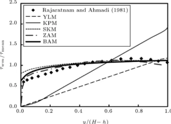
3.3. Shear stress on a main channel wall The shear stress distribution on a main channel wall at h=H = 0:333 in two sections with dierent dimensions is calculated and illustrated in Figures 8 and 9. The results of the ve mentioned methods are compared with the experimental results of Myers and Elsawy [26] and Rajaratnam and Ahmadi [25]. As seen in Figures 8 and 9, at similar ow depths and dierent cross section dimensions as well as channel slopes, the prediction of the shear stress values obviously diered among the methods because all mentioned methods are geometri-cal models. The KPM and YLM presented the same linear distribution that did not match experimental data and contained high errors. It should be mentioned
Figure 8. Relative shear stress distribution on a main channel wall (h=H = 0:333).
Figure 9. Relative shear stress distribution on a main channel wall (h=H = 0:333).
that KPM predicted the worst results among the models. ZAM predicted very small shear stress values at the beginning of the channel. A little further from the separation area, the results were almost equal to experimental data for 0:4 < (H h)y < 0:8, and the predicted results were somewhat overestimated. This method presented results closer to experimental data compared with the YLM and KPM models.
SKM made acceptable predictions, but it did not match well with experimental results at the beginning of the section. The BAM model made predictions considerably close to experimental data (especially in Figure 8) and made superior estimations for shear stress distribution at the beginning of the section compared with SKM. In addition, BAM made accurate predictions in the ow separation section as well as the interface of the main channel and oodplain. Experimental data of Rajaratnam and Ahmadi [25] are used for various section dimensions in Figure 9. The same as before, the BAM model presented better results than those of the other four mentioned meth-ods.
Figure 10. Shear stress distribution on the main channel bed (h=H = 0:5).
3.4. Shear stress on the main channel bed The shear stress distribution on the bed of the main channel predicted by the ve introduced models is shown in Figure 10 and compared with Cokljat and Younis' experimental data [27]. Figure 10 indicates that the KPM and YLM models predicted a similar shear stress distribution pattern for the main channel bed that is contrary to laboratorial outcomes. The SKM model predicted a uniform distribution for shear stress, which is better than the KPM and YLM models. The ZAM model was more adapted to experimental data. However, the ZAM model has more equa-tions and parameters for calculating the shear stress on the main channel bed compared with the other methods. It is also more time-consuming and needs much more calculation accuracy. The BAM model presented the most appropriate results for predicting the shear stress distribution on the main channel bed using fewer and simpler equations than the ZAM model.
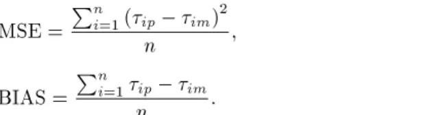
4. Model performance
The performance of the YLM, KPM, SKM, ZAM, and BAM models in predicting the shear stress distribu-tion in compound cross secdistribu-tions is evaluated using statistical comparisons of the predicted and observed outputs. The comparison involves four of the most commonly applied error measures: Root Mean Aquare Error (RMSE), Mean Absolute Percentage of Error (MAPE), Mean Square Error (MSE), and BIAS. These statistical parameters are calculated as:
RMSE = rPn
i=1(ip im)2
n ; (37)
MAPE = 100n1
n
X
i=1
ip im
im
MSE = Pn
i=1(ip im)2
n ; (39)
BIAS = Pn
i=1ip im
n : (40)
Table 1 displays the comparison results between each model and experimental data. YLM with RMSE of 0.442 outperformed KPM with RMSE of 0.556 in estimating the shear stress distribution on a oodplain wall. SKM, ZAM, and BAM produced similar results to some extent. Among all models, ZAM performed better with RMSE=0.045, MAPE=4.12, MSE=0.002, and BIAS=-0.017 (for h=H = 0:25). As seen in Table 1, KPM had lower error values in predicting the shear stress on the bed of main and oodplain channels than YLM. In other words, YLM exhibited higher ability than KPM in predicting the shear stress
distribution on a oodplain wall, and for other sub-sections, KPM outperformed YLM. ZAM predicted the shear stress distribution on a oodplain bed with lower error (RMSE=0.073, MAPE=7.194, MSE=0.005, and BIAS=0.0185) than SKM and BAM, whose average RMSE and average MAPE values were 0.134 and 13.09 also 0.096 and 9.17, respectively. Both methods performed weakly due to the higher error values. The SKM model provided lower statistical parameter values compared with the KPM and YLM models. Considering that secondary ows aect the suggested equations in the ZAM model, ZAM seemed to be more accurate than all other methods. This method could not predict more accurate shear stress values at the interface of the main channel and oodplain, and it predicted the shear stress at the main channel wall with higher error (RMSE of 0.052) compared with BAM and
Table 1. Comparison of experimental results for a compound channel with the results obtained with dierent models. Experiment Subsection h=H Statistical
parameters YLM KPM SKM ZAM BAM
Myers and Elsawy [26]
Wall of oodplain
0.25
RMSE 0.442 0.557 0.069 0.045 0.085 MAPE 41.61 51.84 5.91 4.12 5.18
MSE 0.195 0.310 0.005 0.002 0.007 BIAS -0.24 -0.207 0.046 -0.017 0.043
0.4
RMSE 0.509 0.584 0.026 0.025 0.012 MAPE 46.52 54.41 2.391 1.981 0.557 MSE 0.259 0.341 0.001 0.001 0.000 BIAS -0.13 0.013 -0.014 -0.012 -0.003 Rajaratnam and
Ahmadi [25]
Bed of oodplain
0.5
RMSE 0.277 0.213 0.197 0.076 0.141 MAPE 27.39 20.54 19.12 7.12 13.62 MSE 0.077 0.045 0.039 0.006 0.02 BIAS 0.138 0.006 0.069 0.026 0.023 Myers and
Elsawy [26] 0.325
RMSE 0.511 0.480 0.070 0.070 0.052 MAPE 54.28 48.79 7.055 7.267 4.713 MSE 0.261 0.231 0.005 0.004 0.003 BIAS -0.455 -0.067 0.028 0.011 0.032 Rajaratnam and
Ahmadi [25]
Wall of main channel
0.333
RMSE 0.511 0.480 0.121 0.070 0.089 MAPE 54.28 48.79 11.73 7.267 8.503 MSE 0.261 0.231 0.015 0.004 0.008 BIAS -0.455 -0.067 0.066 0.011 0.0413 Myers and
Elsawy [26] 0.333
RMSE 0.505 0.516 0.091 0.036 0.025 MAPE 48.07 48.57 7.246 3.476 1.802 MSE 0.255 0.266 0.008 0.001 0.001 BIAS -0.439 -0.084 0.058 -0.007 0.014 Cokeljat and
Younis [27]
Bed of
main channel 0.5
RMSE 0.264 0.262 0.063 0.047 0.058 MAPE 24.11 23.78 5.516 4.456 5.266 MSE 0.070 0.068 0.004 0.002 0.003 BIAS -0.005 -0.008 0.021 0.041 0.011
SKM (RMSE of 0.038 and 0.046 respectively). Note that ZAM includes many dependent equations and parameters to estimate shear stress distribution, which necessitates much more time and higher accuracy. The BAM model performed the best in predicting shear stress distribution with smaller values of MAPE% (less than 6%). Compared to the experimental results of Rajaratnam and Ahmadi [25], the BAM model did not produce acceptable results (RMSE of 0.14).
Since ow separation is a parameter with inu-ence on the interface of a main channel and oodplain as well as energy wastage, and the models applied in this study are analytical and geometrical methods; the shear stress values in this region are always predicted as lower than the real values. It should be mentioned that the mean absolute percentage of error with the BAM model is considerably lower than other models in this case. The BAM model can predict shear stress much more accurately than other models even in this case. As seen in Table 1, the statistical parameter values of the BAM and ZAM models are signicantly smaller than other geometrical methods. However, the ZAM model produced good results, but it requires solving many equations for estimating shear stress distribution. On the other hand, the BAM method can estimate shear stress distribution in compound channel sub-sections with high precision and uses simpler and fewer relations than ZAM. It can be deducted that the BAM method is robust in predicting the shear stress distribution along the wetted perimeter of compound channels.
5. Conclusion
The present study expressed ve geometrical and an-alytical models to predict the shear stress distribution in compound channels. These models were compared with experimental data, and the ability of each model in predicting the shear stress in sub-sections of a compound channel was investigated. In four mod-els, the eect of secondary ows on predicting shear stress distribution was ignored, whereas this eect was considered only in ZAM. Based on the obtained results, YLM and KPM predicted the same pattern of shear stress distribution for a oodplain wall and main channel wall, where the shear stress values increased with increasing wetted perimeter. YLM and KPM exhibited poor performance in estimating the shear stress distribution on compound channel walls with average RMSE of 0.49 and 0.53, respectively. Accord-ing to the results, KPM produced adequate results in estimating the shear stress distribution on a oodplain bed with low ow depth. However, with increasing ow depth, the results deviated from the laboratorial outcomes. In fact, KPM estimated the shear stress distribution on a oodplain bed and main channel bed better than YLM. However, both methods were much
weaker in predicting shear stress distribution than the other mentioned methods. The SKM estimations of shear stress distribution for the wetted perimeter of a wall and bed of a oodplain followed a straight line and were close to experimental data for a oodplain wall. For a oodplain bed far from the corners, the SKM results were compatible with laboratorial data. The pattern of shear stress distribution on the wall and bed of a main channel estimated by SKM was more acceptable and the results were better than YLM and KPM. The BAM model performed well in predicting oodplain and main channel shear stress, and it can be deducted that the results for all ow depths are com-patible with laboratorial outcomes. ZAM presented smaller error percentages than the geometric methods pointed out. The ZAM predictions for oodplain and main channel walls at the beginning of the wetted perimeter were much lower than experimental data, but after the beginning point, the estimations were closer to observed data. From all models, the eect of secondary ow was only considered in ZAM, which resulted in a superior performance to other models in predicting shear stress in compound channels. Among the methods in which the eect of secondary ow was ignored, BAM performed most appropriately. It is deducted that both BAM and ZAM are more accurate than other models, with mean RMSE of 0.058, and 0.049, respectively. It is noted that in the BAM model, solving implicit equations is required to compute the Lagrange multipliers. On the other hand, ZAM calls for solving several equations for predicting shear stress in compound channels, it is time-consuming and re-quires high accuracy. In this regard, the BAM model necessitates fewer equations. Therefore, BAM may be selected as the most suitable model for estimating the shear stress distribution in compound channels among the models presented in this study. The authors of the present study investigated a novel, simpler equation to avoid solving implicit equations in BAM for predicting shear stress distribution with high precision.
References
1. Knight, D.W., Yuen, K.W.H. and Al Hamid, A.A.I. \Boundary shear stress distributions in open channel ow", In: K. Beven, P. Chatwin, and J. Millbank (eds), Physical Mechanisms of Mixing and Transport in the Environment, Wiley New York, pp. 51-87 (1994). 2. Prasad, B.V.R. and Manson, J.R. \Discussion of a
geometrical method for computing the distribution of boundary shear stress across irregular straight open channels", J. Hydraul. Res., 40(4), pp. 537-539 (2002). 3. Guo, J. and Julien, P.Y. \Shear stress in smooth rect-angular open-channel ow", J. Hydraul. Eng., 131(1), pp. 30-37 (2005).
of stable channels by the bureau of reclamation", J. Hydraul. Div., 79(280), pp. 1-30 (1953).
5. Cruf, R.W. \Cross section transfer of linear momen-tum in smooth rectangular channel", Geological Survey Water Supply paper 1592-B, U.S. Government Printing Oce, Washington D.C. (1965).
6. Myers, W.R.C. \Momentum transfer in a compound channel", J. Hydraul. Res., 16(2), pp. 139-150 (1978). 7. Yuen, K.W.H. \A study of boundary shear stress, ow resistance and momentum transfer in open channels with simple and trapezoidal cross section", PhD The-sis, The University of Birmingham (1989).
8. Knight, D.W. and Sterling, M. \Boundary shear in circular pipes partially full", J. Hydraul. Eng., 126(4), pp. 263-275 (2000).
9. Seckin, G., Seckin, N. and Yurtal, R. \Boundary shear stress analysis in smooth rectangular channels", Can. J. Civil Eng., 33, pp. 336-342 (2006).
10. Yang, S.Q. and Lim, S.Y. \Mechanism of energy transportation and turbulent ow in a 3D channel", J. Hydraul. Eng., 123(8), pp. 684-692 (1997). 11. Khodashenas, S.R. and Paquier, A. \A geometrical
method for computing the distribution of boundary shear stress across irregular straight open channel", J. Hydraul. Res., 37, pp. 381-388 (1999).
12. Sterling, M. and Knight, D.W. \An attempt at using the entropy approach to predict the transverse distri-bution of boundary shear stress in open channel ow", Stoch. Env. Res. Risk Assess., 16, pp. 127-142 (2002). 13. Berlamont, J.E., Trouw, K. and Luyckx, G. \Shear stress distribution in partially lled pipes", J. Hydraul. Eng., 129(9), pp. 697-705 (2003).
14. Yang, S.Q. and Lim, S.Y. \Boundary shear stress distribution in trapezoidal channels", J. Hydraul. Res., 43(1), pp. 98-102 (2005).
15. Bonakdari, H., Larrarte, F. and Joannis, C. \Study of shear stress in narrow channels: application to sewers", Urban Water, 5(1), pp. 15-20 (2008).
16. El Kadi Abderrezzak, K. \Evolution of the riverbed due to ow and sediment transport", PhD Thesis, University of Claude Bernard, Lyon (2006).
17. Javid, S. and Mohammadi, M. \Boundary shear stress in a trapezoidal channel", Int. J. Eng., 25(4), pp. 365-373 (2012).
18. Kabiri-Samani, A., Farshi, F. and Chamani, M.R. \Boundary shear stress in smooth trapezoidal open channel ows", J. Hydraul. Eng., 139(2), pp. 205-212 (2013).
19. Bonakdari, H., Sheikh, Z. and Tooshmalani, M. \Com-parison between Shannon and Tsallis entropies for prediction of shear stress distribution in circular open channels", Stoch. Env. Res. Risk Assess., 29(1), pp. 1-11 (2015).
20. Bonakdari, H., Tooshmalani, M. and Sheikh, Z. \Predicting shear stress distribution in rectangular channels using entropy concept", Int. J. Eng., 28(3), pp. 360-367 (2015).
21. Sheikh, Z. and Bonakdari, H. \Prediction of boundary shear stress in circular and trapezoidal channels with entropy concept", Urban Water, 13(6), pp. 629-636 (2015).
22. Chiu, C.L. \Application of entropy concept in open channel ows", J. Hydraul. Eng., 117(5), pp. 615-628 (1991).
23. Araujo, J.C. and Chaudhry, F.H. \Experimental eval-uation of 2-D entropy model for open channel ow", J. Hydraul. Eng., 124(10), pp. 1064-1067 (1998). 24. Zarrati, A.R., Jin, Y.C. and Karimpour, S.
\Semiana-lytical model for shear stress distribution in simple and compound open channels", J. Hydraul. Eng., 134(2), pp. 205-215 (2008).
25. Rajaratnam, N. and Ahmadi, R. \Hydraulics of chan-nels with ood-plains", J. Hydraul. Res., 19(1), pp. 43-60 (1981).
26. Myers, W.R.C. and Elsawy, E.M. \Boundary shear in channel with ood-plain", J. Hydraul. Div., 101(7), pp. 933-946 (1975).
27. Cokljat, D. and Younis, B.A. \Second-order clo-sure study of open-channel ows", J. Hydraul. Eng., 121(2), pp. 94-107 (1995).
Biographies
Zohreh Sheikh Khozani is now PhD candidate in Hydraulic structures (Civil Engineering), Faculty of Engineering, University of Razi, Kermanshah, Iran. She obtained MSc degree from Semnan University in 2011. She has 6 published papers in ISI journals and more than 4 conference presentations. She works in eld of shear stress distribution, sediment transport in open channels and rivers, and use of entropy concept and soft computing methods in engineering applica-tions.
Hossein Bonakdari is a Professor, Department of Civil Engineering of University of Razi, earned his PhD in Civil Engineering in the University of Caen-France. He has spent his MSc in civil engineering, hydraulics structures in University of Ferdowsi, Mash-had, Iran. His elds of specialization and interest include metrology and modeling of wastewater urban drainage systems, soft computing, sediment transport, computational uid dynamic and hydraulics, design of hydraulic structures, and uid mechanics. From 2010 till 2011, he has been a researcher at Laboratory of Civil and Environmental Engineering, INSA of Lyon, France. Results obtained from his researches have been published in more than 65 papers in international journals (h-index=8). He has also more than 150 presentations in national and international conferences. He published two books.
![Figure 3. Geometric parameters of a compound channel [24].](https://thumb-us.123doks.com/thumbv2/123dok_us/8380511.2226381/4.892.480.827.206.384/figure-geometric-parameters-compound-channel.webp)