DEVELOPMENT OF A STATIONARY CHEST TOMOSYNTHESIS SYSTEM USING CARBON NANOTUBE X-RAY SOURCE ARRAY
Jing Shan
A dissertation submitted to the faculty at the University of North Carolina at Chapel Hill in partial fulfillment of the requirements for the degree of Doctor of Philosophy in the
Department of Physics and Astronomy (Physics).
Chapel Hill 2015
c 2015 Jing Shan
ABSTRACT
Jing Shan: Development of a stationary chest tomosynthesis system using carbon nanotube x-ray source array
(Under the direction of Otto Zhou)
X-ray imaging system has shown its usefulness for providing quick and easy access of imaging in both clinic settings and emergency situations. It greatly improves the workflow in hospitals. However, the conventional radiography systems, lacks 3D information in the images. The tissue overlapping issue in the 2D projection image result in low sensitivity and specificity. Both computed tomography and digital tomosynthesis, the two conventional 3D imaging modalities, requires a complex gantry to mechanically translate the x-ray source to various positions.
Over the past decade, our research group has developed a carbon nanotube (CNT) based x-ray source technology. The CNT x-ray sources allows compacting multiple x-ray sources into a single x-ray tube. Each individual x-ray source in the source array can be electronically switched. This technology allows development of stationary tomographic imaging modalities without any complex mechanical gantries. The goal of this work is to develop a stationary digital chest tomosynthesis (s-DCT) system, and implement it for a clinical trial.
ACKNOWLEDGEMENTS
First and foremost, I am deeply grateful to my advisor, Dr. Otto Zhou for his guidance and encouragement throughout my graduate studies. His enthusiasm and dedication in translating research to useful applications has truly inspired me. I also highly appreciate all the members in my committee, Dr. David Lalush, Dr. Yueh Z. Lee, Dr. Jianping Lu, Dr. Xiaohui Wang, and Dr. Sean Washburn for their their guidance and advice. Particular thanks goes to Dr. Jianping Lu, and Dr. Yueh Z. Lee for helpful insights and guidance into my research. I would also like to thank each member of our research group, past and present, that has helped me through my researches and studies, including: Laurel Burk, Jabari Calliste, Guohua Cao, Pavel Chtcheprov, Emily Gidcumb, Mike Hadsell, Allison Hartman, Christy Inscoe, Marci Potuzko, Xin Qian, Shabana Sultana, Jiong Wang, Gongting Wu, Guang Yang, Jerry Zhang, and Lei Zhang.
TABLE OF CONTENTS
LIST OF TABLES . . . xiv
LIST OF FIGURES . . . xvi
LIST OF ABBREVIATIONS AND SYMBOLS . . . xxx
1 Introduction . . . 1
1.1 Dissertation Overview . . . 1
1.2 Specific Research Aims . . . 3
1.2.1 Feasibility of s-DCT . . . 3
1.2.2 Integration of s-DCT for Clinical Use . . . 3
1.2.3 Investigation of Imaging Parameters and Imaging Protocols . . . 3
1.3 Dissertation Organization . . . 4
2 X-rays . . . 5
2.1 Discovery of X-rays . . . 5
2.2 Interactions with Matter . . . 5
2.2.1 Photoelectric Absorption . . . 6
2.2.2 Rayleigh Scattering . . . 9
2.2.3 Compton Scattering . . . 9
2.2.4 Pair Production . . . 10
2.3 X-ray Attenuation . . . 11
2.4 Generation of X-ray . . . 12
2.4.1 Bremsstrahlung Radiation . . . 12
2.4.2 Characteristic X-rays . . . 12
2.4.3 Synchrotron Radiation . . . 13
2.5 X-ray Tubes . . . 15
2.5.1 Cathode . . . 15
2.5.2 Anode . . . 16
2.5.3 Focal Spot . . . 17
2.5.4 Tube Housing and Filtration . . . 17
3 Digital Chest Tomosynthesis . . . 21
3.1 X-ray Imaging Modalities for Chest . . . 21
3.1.1 Chest X-ray Radiography . . . 21
3.1.2 Computed Tomography . . . 22
3.1.3 Digital Chest Tomosynthesis . . . 23
3.2 Digital Tomosynthesis . . . 23
3.2.1 Principles of Chest Tomosynthesis . . . 23
3.2.2 Commercial DCT Systems . . . 25
3.2.3 Dosimetry of DCT Systems . . . 28
3.2.5 Limitations of Conventional DCT . . . 29
4 Carbon Nanotube X-ray Source . . . 30
4.1 Carbon Nanotube . . . 30
4.2 CNT Based Field Emission X-ray Source . . . 30
4.2.1 Field Emission Effect . . . 30
4.2.2 X-ray Source Using CNT Field Emitters . . . 32
4.3 CNT X-ray Source Applications . . . 35
4.3.1 Micro-CT . . . 35
4.3.2 s-DBT . . . 37
4.3.3 Stationary CT . . . 37
4.3.4 MRT . . . 38
5 Feasibility of a Stationary Chest Tomosynthesis System Using CNT Source Array . . . 40
5.1 Overview . . . 40
5.2 Purpose . . . 41
5.3 Materials and Methods . . . 42
5.3.1 Distributed CNT X-ray Source Array . . . 43
5.3.2 System Description . . . 44
5.3.3 X-ray Output and Beam Quality . . . 46
5.3.4 Image Reconstruction . . . 47
5.3.5 The System MTF and ASF . . . 48
5.4 Results . . . 49
5.4.1 CNT X-ray Source Array Characterization . . . 49
5.4.2 Focal Spot Size . . . 52
5.4.3 Beam Quality . . . 54
5.4.4 Radiation Dose . . . 54
5.4.5 System MTF and ASF . . . 55
5.4.6 Phantom Imaging . . . 57
5.5 Discussions . . . 60
5.6 Summary . . . 62
6 Characterization of s-DCT and Related Physics Problems . . . 64
6.1 Overview . . . 64
6.2 Source Stability . . . 64
6.2.1 Purpose . . . 64
6.2.2 Methods . . . 65
6.2.3 Results: Stability of the x-ray pulse . . . 66
6.2.4 Results: Long term stability of CNT x-ray sources . . . 67
6.2.5 Discussion and Conclusion . . . 73
6.3 Extra-focal Radiation of the s-DCT . . . 74
6.3.1 Purpose . . . 74
6.3.2 Methods . . . 76
6.3.3 Results . . . 85
6.4 Anode Thermal Analysis . . . 103
6.4.1 Introduction . . . 103
6.4.2 Simulation Model . . . 104
6.4.3 Validation of the Model . . . 106
6.4.4 Anode heat simulation for CNT micro-CT . . . 107
6.4.5 Anode heat simulation for s-DBT and s-DCT systems . . . 112
6.4.6 Anode heat simulation for MRT system . . . 115
6.4.7 Conclusions . . . 117
6.5 CNT Source Array Geometry Calibration . . . 117
6.5.1 Introduction . . . 117
6.5.2 Geometry calibration method . . . 118
6.5.3 Geometry calibration phantom . . . 119
6.5.4 A statistical model based optimization method . . . 123
6.5.5 Comparison of the two calibration methods . . . 127
6.5.6 Discussion . . . 128
7 Evaluation of imaging geometries for the s-DCT system . . . 131
7.1 Overview . . . 131
7.2 Purpose . . . 131
7.3 Methods . . . 132
7.3.1 System Descriptions . . . 132
7.3.2 Imaging Geometries . . . 132
7.3.4 Anthropomorphic Phantom Images . . . 134
7.4 Results . . . 135
7.4.1 System MTF and ASF for All Imaging Geometries . . . 135
7.4.2 Anthropomorphic phantom Imaging . . . 136
7.5 Discussion . . . 136
8 Prospectively Gated s-DCT . . . 139
8.1 Overview . . . 139
8.2 Purpose . . . 139
8.3 Methods . . . 140
8.3.1 System Description . . . 140
8.3.2 Dynamic Phantom . . . 142
8.3.3 Physiologically Gated Tomosynthesis . . . 142
8.4 Results . . . 144
8.4.1 CNT X-ray Source Array . . . 144
8.4.2 Physiologically Gated Tomosynthesis imaging . . . 145
8.5 Discussion . . . 146
8.6 Conclusion . . . 148
9 Applications of s-DCT and Techniques to Improve Image Quality . . . . 149
9.1 Overview . . . 149
9.2 Using s-DCT as Diagnosis and Monitoring Tools in Pediatric Cystic Fibrosis Patients . . . 149
9.2.2 Methods . . . 150
9.2.3 Results . . . 151
9.2.4 Discussion and Conclusion . . . 151
9.3 A Scatter Reduction Technique for s-DCT . . . 152
9.3.1 Purpose . . . 152
9.3.2 Methods . . . 153
9.3.3 Results . . . 157
9.3.4 Discussions and Conclusions . . . 159
10 Clinical Implementation of an s-DCT Prototype . . . 161
10.1 Overview . . . 161
10.2 Construction of the Prototype s-DCT . . . 161
10.3 Software for the s-DCT . . . 163
10.4 Patient and Operator Safety . . . 163
10.4.1 Electrical Safety . . . 165
10.4.2 Radiation Safety . . . 167
10.5 Workflow of s-DCT . . . 169
10.5.1 Patient Check-in . . . 170
10.5.2 Patient Positioning . . . 171
10.5.3 Acquiring the Scout View . . . 172
10.5.4 Acquiring Tomosynthesis Images . . . 173
10.5.5 Image Handling and Reconstruction . . . 173
10.7 Conclusion . . . 174
11 Summary and Future Directions . . . 176
11.1 Summary . . . 176
11.2 Future Directions . . . 177
LIST OF TABLES
2.1 Excerpts of FDA HVL regulations for an x-ray tube operated
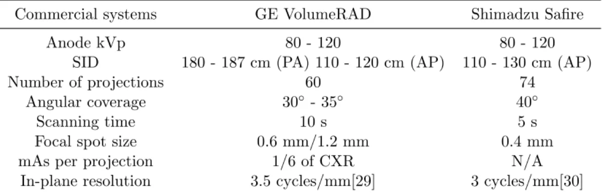
between 60 kVp and 120 kVp. . . 19 3.1 List of key specs of the commercial DCT systems. . . 27 3.2 Comparison of CXR, DCT and CT for detection of lung
nod-ules with CT as reference . . . 29 5.1 The experimentally measured MTF and ASF of the bench-top
chest tomosynthesis system for three different angular spans. M T Fx refers to direction parallel to the scanning direction,
and M T Fy refers to the perpendicular direction. . . 57 6.1 Focal spot size measured at 80 kVp with various anode current. . . 77 6.2 Focal spot size measured at 5 mA current at various anode voltages. . . 77 6.3 w2 for various collimator magnification factor M ag using ideal collimator . . 86 6.4 w2 for various collimator magnification factor,M ag, using 1/4
in lead collimator . . . 87 6.5 w2 for various collimator magnification factors, M ag, using
1/2 in tungsten collimator . . . 89 6.6 Measuredw2 for dose to drop to the 10−1 order and 10−2 order
in the x direction. . . 90 6.7 Comparison of the experimentally measuredw2and simulated
w2 using both simulation models. . . 91 6.8 Summary of measured noise in the dark field images. . . 93 6.9 Simulated anode maximum temperature for 0.6 mm×0.6 mm
FWHM focal spot size at various conditions. . . 113 6.10 Estimation of s-DCT operating conditions based on anode
heat load simulation. . . 115 7.1 MTFs and FWHM of ASF measurements for linear imaging
7.2 MTFs and FWHM of ASF measurements for non-linear
LIST OF FIGURES
2.1 X-ray photograph of the hand of R¨ontgen’s wife. . . 6 2.2 Illustration of ray and matter interactions. (A) Most
x-ray photons have no interaction with the material, passing through unattenuated. (B) Photoelectric absorption results in total removal of the x-ray photon and production of a pho-toelectron, and a characteristic x-ray. (C) Elastic Rayleigh scattering with small change of trajectory of the x-ray pho-ton. (D) Compton scattering between high energy photons and less bounded electrons. Scattering photon with less
en-ergy and a recoiled electron are generated. . . 7 2.3 Illustration of photoelectric effect. (a) Photon absorption and
ejection of photoelectron. (b) Characteristic x-ray emission. . . 8 2.4 Illustration of the Bremsstrahlung radiation. An electron is
deflected when passing by the nucleus of an atom, the loss of
kinetic energy transfers to the x-ray photon. . . 13 2.5 Energy spectrum of x-rays generated using a 90 kVp tube.
The characteristic lines Kα1, Kα2, and Kβ1 are marked. . . 14 2.6 Synchrotron radiation from the bending charged beam. The
radiation beam is sharply collimated forward. . . 14 2.7 Diagram of a Coolidge tube. The major component of the
tube is the cathode, the anode, and the tube housing. . . 15 2.8 Illustration of the field of view and effective focal spot with
respect to anode angle. . . 18 2.9 Illustration of the effect of x-ray tube filtration on x-ray
spec-trum. (a) Shows the unfiltered Bremsstrahlung spectrum with great low-energy x-ray photon production. (b) Shows the fil-tered spectrum with preferential attenuation on the low
en-ergy photons. . . 19 3.1 Illustration of a DCT system. The system consists of a
com-puter controlled gantry that can move the x-ray source to various locations long a vertical path, a flat panel detector,
3.2 Shift-and-add technique for tomosynthesis image reconstruc-tion. In this illustration, five projection views are used for tomosynthesis reconstruction. The five images are shifted and added to yield composite images at two different planes.
Dif-ferent objects come in focus at difDif-ferent imaging planes. . . 25 3.3 Illustration and photo of GE VolumeRAD DCT system. . . 26 3.4 Illustration of Shimadzu SONIALVISION DCT system. . . 27 4.1 Illustration of the field emission effect. The application of the
electric field lowers the effective barrier so electrons near the
Fermi level can tunnel through the barrier. . . 32 4.2 (a) Schematic of the triode-type field emission x-ray tube. (b)
X-ray images of a fish and human hand phantom taken using
the CNT x-ray source. . . 33 4.3 Schematic of the typical CNT source design. The source
con-sists of a CNT cathode, gate and focusing electrodes, and anode. The anode has high voltage applied, while a smaller voltage (in the order of 1000 V) is applied between the gate and cathode. The blue box shows a picture of a representative cathode surface with CNTs, captured by scanning electron
microscope (SEM). . . 34 4.4 Micro-CT using a CNT based x-ray source. (a) System setup
of the micro-CT. The inset shows the system with the cover and shielding. (b) Reconstructions of the micro-CT datasets
of a mouse gated to both cardiac and respiration cycles. . . 36 4.5 A photo of the s-DBT system under clinical evaluation in the
N.C. Cancer hospital. . . 37 4.6 Desktop micro-beam radiation therapy system using CNT
x-ray sources. (a) The picture of the system setup. (b) A his-tological slice of a mouse brain showing the DNA damage of
tumor cells by the micro-beam. . . 38 5.1 Bench-top stationary chest tomosynthesis system. The linear
CNT x-ray source array consists of 75 x-ray generating fo-cal spots. The detector and phantom, mounted on the same
5.2 Timing diagram for s-DCT imaging. Computer generates a trigger signal to externally trigger the detector. The detector ready-to-exposure signal is synced to the x-ray source switch-ing system, where each pulse will be used to trigger a sswitch-ingle CNT x-ray source in the source array. The CNT sources are
fired in a sequence preset by the operator. . . 45 5.3 An illustration of the imaging geometry in the bench top
sta-tionary chest tomosynthesis system. The source-to-detector distance is 110 cm. By moving the detector and phantom to-gether, parallel to the source array, we were able to emulate different imaging geometries. In the current bench-top proof-of-concept setup, the effective x-ray source array is able to cover up to a 34◦ angular span relative to the detector center
with up to 85 projections. . . 46 5.4 An example of CNT cathode performance in the x-ray tube.
(a) The I-V curve of a CNT cathode shows the voltage needed to extract 7.5 mA of current. (b) The anode current wave-forms for 5 mA current and 33 ms pulse width from 5 different CNT sources. The overshot signal at the beginning of each pulse was the step response of the switching electronics, which
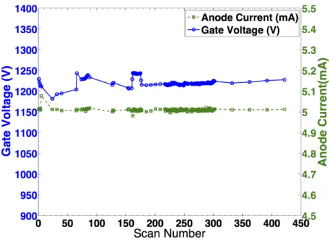
was not a real anode current overshoot. . . 49 5.5 Stability measurement of a CNT source over 400 scans during
a 4 month period. The tube current (green dashed curve) was kept at 5 mA, the cathode-gate voltage (blue curve) barely changes in the test. The tube current fluctuation is less than 2% over the 400 scans, and no significant
degrada-tion of cathode-gate voltage was observed. . . 50 5.6 Cathode-gate voltages needed to generate 5 mA tube current
from each cathode. All 75 CNT cathodes can generate the desired current, with a small variation in voltage from cathode to cathode. The average voltage needed is 1240 V. The P00 refers to the central beam source, while the P and N notate positive and negative locations of the source relative to the
central beam, respectively. . . 51 5.7 Summary of anode current in a short tomosynthesis scan using
32 sources and the relative difference to the average anode current. The CNT source array consistently output 5 mA
5.8 Focal spot measurement using a pinhole. (a) shows the a typical pinhole image acquired at 80 kVp and 5 mA. The pinhole was 400µm in diameter and 2 mm in thickness. (b) shows the normalized intensity and the 2D Gaussian fit of the
focal spot distribution. . . 52 5.9 Summary of the focal spot size measurement of 5 sources in
the source array. The average focal spot size was measured to be 2.5 mm× 0.5 mm. The results show a good source-to-source consistency, as the relative difference is less than
4%. . . 53 5.10 Normalized intensity in log 2 scale versus the thickness of
ad-ditional aluminum filtration. The first HVL was determined by finding the thickness of aluminum to halve the dose. The
first HVL of this source array was measured to be 3 mm at 80 kVp. . . 54 5.11 Experimentally measured relation between the incident air
kerma at 100 cm from focal spot and x-ray tube output (mAs). The air kerma is linear to the anode output. The incident air
kerma per mAs at 100 cm was measured as 74.47 µGymAs−1. . . . 55 5.12 (a) A reconstructed cross wire phantom in the plane of
fo-cus with an angular coverage of 34◦. The region outlined by the red box illustrates one randomly selected ROI used to calculate the ASF. (b) The LSF of the horizontal tung-sten wire and the Gaussian-fitted LSF from the 34◦ angular coverage dataset. (c) The MTFs of the system in both x (1.5 cycles/mm) andy (3.2 cycles/mm) directions for the 34◦ dataset. (d) The ASF of the system measured in the 34◦ dataset. The measured FWHM of the ASF indicates a 5.2
mm z-axis resolution. . . 56 5.13 (a) and (d) show two slices at different depth (separate by 2.4
cm) reconstructed from 29 projection images acquired over 11.6◦, (b) and (e), and (c) and (f) show the same slices re-constructed with same number of projection images but with 23◦ and 34◦ angular coverage, respectively. All three sets of images were acquired at the same total dose. It can be seen that the wider the angular coverage the lesser is the out of plan tomo artifact (such as those from the rib cage), due to
5.14 (a) shows a slice reconstructed with 29 projections over 34◦ angular span, while (c) shows the same slice reconstructed with 85 projections over the same angular span. As shown in the zoomed in region, outlined with a red box in (b) and (d), it can be seen that the ripple artifacts decreased when the number of projection images is increased. The two sets of
images were acquired at the same total dose. . . 59
6.1 The tube current waveform for a 150 ms pulse. The current was set to output 5 mA. The waveform shows stable current output and accurate timing. . . 66
6.2 The tube current waveform for 5 mA current and 33 ms pulse width from 5 different CNT sources. The waveforms demon-strate the consistency between sources. . . 67
6.3 Stability measure for source #11. . . 68
6.4 Stability measure for source #20. Source 20 is the most used source in the source array, with over 9,900 scans and accumu-lated output of 1,575 mAs. . . 69
6.5 Stability measure for source #24. . . 70
6.6 Stability measure for source #29. . . 71
6.7 Stability measure for source #35. . . 72
6.8 SEM image of a CNT cathode typically used in CNT x-ray sources. . . 74
6.9 Zone of intersection of all straight lines that pass through all radiation apertures of the x-ray source assembly, with a plane normal to the reference axis at 1m from the focal spot shall not extend more than 15 cm outside the boundary of the largest selectable X-ray field. . . 75
6.11 Simulation geometry. The source-to-detector distance was 1000 mm. A collimator was put between the source and detec-tor to collimate the beam right to the detecdetec-tor. The source-to-collimator distance wasn, while the collimator-to-detector
distance was m. . . 79 6.12 The focal spot was sampled into small bins, the intensity of
each bin determined from the focal spot intensity of the
Gaus-sian distribution. . . 80 6.13 Attenuation coefficient of lead. Source: NIST database . . . 82 6.14 Experimental extra-focal radiation measurement setup. A
lead sheet was put in front of the tube window, a square aper-ture was open to collimate x-ray beams. Two 12.7 mm (0.5 in) thick tungsten block were placed in front of the aperture as extra collimator along x-direction, due to the longer focal spot size in x-direction. The opening between tungsten block
was 5 mm. . . 84 6.15 (a) Normalized dose profile on the detector plane, the
detec-tor width is 400mm, the collimator magnification factorM ag is 25, which is close to realistic design. With higher magnifi-cation, the intensity drops more slowly off the detector edge. (b) The normalized dose intensity plotted in log scale. The plot suggests the extra-focal radiation drops to the 10−3 order
within 76.6mm, which is less than the required 15 cm. . . 85 6.16 Normalized dose profile forM ag = 30, the dose drops to 10−3
order in 91.9 mm, which is less than the 15cm requirement. . . 86 6.17 (a) Extra-focal radiation dose profile for M ag = 25 with 1/4
in lead collimator. The w2 is 131.8 mm, which is less than the 15 cm requirement. (b) Comparison of ”Ideal” collimator and ”real” collimator for M ag = 25. The blue curve shows the simulated dose profile with ”ideal” collimator, which can block all x-rays. The green curve shows the simulated profile with a 6.35 mm lead collimator with 80 keV monochromatic x-rays. The ”real” scenario shows slower dose drop. However,
6.18 (a) Projection image of the lead collimator. The dose profile along the x-direction was measured, as marked by the red line. (b) The raw pixel number profile of the collimator image along
the x-direction (the red line shown in (a)). . . 90 6.19 Experimentally measured normalized dose profile plotted in
log scale. The dose does not drop to the expected 10−3 order. . . . 91 6.20 (a) Experimentally measured dose profile in the x-direction.
The dose drop rate decreases dramatically at approximately 10−1.5 order. (b) Simulated dose profile using an ideal col-limator (Model M0) for the same condition. (c) Simulated dose profile using a 13.7 mm tungsten collimator, and 80 keV
monochromatic x-rays (Model M1). . . 92 6.21 (a) Subtraction image of the leakage radiation. The bright
collimated area shows the leakage radiation. The red arrow marks the analyzed line profile. (b) A line profile across the
collimated area. The leakage radiation contributes little radiation. . . 95 6.22 (a) Illustration of the penumbra effect caused by the
collima-tor. (b) A simulation with a low attenuation collimacollima-tor. . . 96 6.23 Illustration of the experiment to evaluate scattered x-rays.
The collimator was aligned to source 20, which is located roughly in the center of the source array. By firing source 20, the primary beam (red line) will pass through the colli-mator and shine on the detector. The primary beam and the scattered x-rays mix together, thus it is hard to measure the scattered x-rays. But by firing source 26, which is 48 mm away from source 20, the primary beam and scattered x-rays can be separated. The primary beam of source 26 (dark blue line) is∼55 cm away from the center of the detector based on a simple geometry calculation. But the scattered x-ray (blue
dashed line) can reach the detector and can be measured. . . 97 6.24 Projection image of scattered image of source 2. The image
is similar to the leakage radiation image since the scattered
signal is much less than the leakage radiation . . . 98 6.25 (a)Scatter x-ray image of source 26. The bright band in
the image is due to the scatter radiation from the collima-tor edge. (b) Intensity profiles along the x-direction (blue)
6.26 By changing the relative position of the focal spot and colli-mator opening, the scatter intensity on the top and bottom edge will change. Initially, the focal spot F is aligned better with the top edge, therefore there is less scatter off the top edge. By gradually moving the collimator up, the focal spot moves to F’ relative to the collimator, and the scatter off the top edge will increase while the scatter from the bottom edge
will decrease. . . 100 6.27 (a) Projection image of the collimated area with source 26
fired. The image shows the scattered x-ray intensity. The collimator was moved up 2 mm. (b) The line profile across x- (blue) and y- (red) direction for figure (a). (c) Scattering x-ray image with collimator moved up for 4 mm. (d) The line
profile along x- and y- direction for figure (c). . . 102 6.28 Schematic of the structure of the CNT based field emission
micro-focused x-ray tube and the demonstration of the
tem-perature distribution on the anode surface. . . 105 6.29 Temperature dependence of the thermal diffusivity, thermal
conductivity, and heat capacity of tungsten. The thermal conductivity decreases with the temperature while the heat capacity increases with the temperature, thus the thermal dif-fusivity decreases from 0.66 cm2/s at 300 K to 2.4 cm2/s at 3000 K. It is important to include the temperature depen-dency of both the thermal conductivity and heat capacity in
anode thermal analysis. . . 106 6.30 Comparison of electron beam melting radius in the
micro-focus tube between simulated and experimental results. The open symbols with fitted smooth lines are simulation results; the scattered solid points are experimental results. The agree-ment between simulated and experiagree-mental results suggests that the simulation is reliable for investigating thermal
load-ing of the anode. . . 108 6.31 Maximum power of a micro focus CNT x-ray tube as a
func-tion of effective focal spot size for a 10◦ tungsten anode. In DC mode, the simulated results agree well with Flynn’s em-pirical formula (dashed curve). However, in pulsed mode, the
6.32 Maximum power of an x-ray tube running in DC mode as a function of effective focal spot size at 6◦, 10◦, and 20◦ anode angles. The maximum power in DC mode is a power function of effective focal spot size, P =kf0.73
s , where the coefficientk is a linear function of e, k = 0.24e+ 1.64. Simulated results suggest that the maximum power is related to the anode angle in DC operation mode; the smaller the anode angle, the higher
power the x-ray tube can apply. . . 111 6.33 Maximum temperature over time in a 10 ms pulse. The
tem-perature both rises and drops rapidly when the electron beam is turned on or off. This result suggests heat can be dissipated very quickly in pulsed mode with low duty cycle. Thus, the tube can be operated at a significantly higher power than that
in DC mode. . . 112 6.34 Maximum power of CNT micro-CT x-ray tube running in
pulsed mode as a function of effective focal spot size, with anode angles at 6◦, 10◦, and 20◦. Simulation results suggest the maximum power for pulsed mode linearly increases with
focal spot size, and can be described by a simple scaling law. . . 113 6.35 The simulated temperature profile over time at the center of
the focal spot during a single x-ray exposure at three different power levels. The dashed horizontal line indicates 80% of the melting temperature of tungsten. The insert shows the temperature distribution on the anode surface for the 38 kVp,
28 mA, 250 ms exposure. . . 114 6.36 Anode temperature distribution for MRT system operated at
160 kVp, 35 mA, 1 s pulse width. . . 115 6.37 Anode temperature distribution in the cross-section for the
MRT system operated at 160 kVp, 35 mA, 1 s pulse width. . . 116 6.38 Anode maximum temperature profile for the MRT system at
various tube currents. . . 116 6.39 Illustration of the geometry calibration method. F denotes
the position of the focal spot. Metal beads (ideal point) A, B, C, D, H, I, J, and K are placed in the image field, and projected images of the beads are atA0,B0,C0,D0,H0,I0,J0,
6.40 CAD drawing of the geometry calibration phantom. The phantom has two acrylic sheets parallel to each other. Four tungsten bars were placed perpendicular to the acrylic layer.
Each acrylic plate had four metal beads embedded inside. . . 120 6.41 An example projection image of the geometry calibration
phan-tom. Yellow lines are the centerlines of the four vertical tung-sten bars. The intersection point of these four lines gives the x, and y coordinates of the focal spot. The distance between metal beads can be used to calculate the magnification factor M1 and M2 for the top and bottom layer of the phantom.
Thus, thez coordinate of the focal spot can be calculated. . . 121 6.42 Illustration of the source of error using average coordinates of
all intersection points to estimate the focal spot’s xand y coordinates. . . . 122 6.43 Illustration of the source of error in an extreme case using
average coordinates of all intersection points as focal spot x andypositions. The intersection point ofl1 andl2 is far away from other intersection points due to the small angle between
l1 and l2. The averaged point, Pavg, produces a large error. . . 123 6.44 Illustration of the physical meaning of the optimization method. . . 126 6.45 The geometry calibration results of the xcoordinates of focal
spots in the s-DCT source array, using mean value method and optimization method. The optimization method shows
better calibration accuracy. . . 127 6.46 Comparison of the geometry calibration results of the y
co-ordinates between the mean value method and optimization method. The optimization method shows better calibration
accuracy. . . 128 6.47 An image of a metal bead used in the geometry calibration
procedure. The blurred edge of the bead increases uncertainty
in edge detection and feature recognition of the image. . . 129 7.1 The s-DCT system consists a linear CNT source array, a flat
panel detector, a phantom and translation stages. The detec-tor and phantom can be simultaneously translated to simulate
7.2 Imaging geometry configuration studied. All imaging config-urations are using same SID of 1100 mm. A linear imaging geometry with angular span of 11.6◦, 23◦,and 34◦, a square ge-ometry centered with detector center and 10◦ angular span on each side, a rectangular geometry with 13.3◦ and 10◦ angular coverage along x and y direction, and a circular geometry with 10◦ angular coverage are studied. The x-direction is along the source array scanning direction, which is also corresponding to the phantom spine direction, while the y-direction is de-fined as perpendicular to the scanning direction, as noted in
both figures. . . 134 7.3 Comparisons of tomosynthesis reconstructed using projection
images acquired with 11.6◦ and 34◦ angular coverage in linear geometry. Both slices clearly show airways and detailed vas-cular structures inside the phantom. The wider (34◦) angular
coverage results in better reduction of out-of-plane artifacts of ribs. . . 137 7.4 Comparison of tomosynthesis slices of linear imaging
geom-etry and square imaging geomgeom-etry with comparable angular coverage. The slice of square imaging geometry shows more fine structures along x direction and better reduction of
arti-facts of ribs from other slices. . . 138 8.1 Stationary chest tomosynthesis system consisting of a CNT
source array, a flat panel detector and an anthropomorphic phantom mounted on the same translation stage. The source array contains 75 focal spots, and has a 298 mm end-to-end length. The detector is 30 cm×30 cm, and can acquire images
at up to 30f ps in the 2×2 binning mode. . . 141 8.2 Timing graph of physiologically gated s-DCT. In this study,
the detector ready to exposure signal is filtered by the phys-iological signal captured by the Bio Vet sensor. The x-ray
source only fires when the lung is in a certain respiration phase. . . 142 8.3 (a) Mechanical ventilator used for the dynamic phantom. The
ventilation speed (bpm) and volume per ventilation (percent-age of lung volume) can be adjusted to simulate various respi-ration patterns. (b) The dynamic phantom. Porcine lung and heart block were placed inside the anthropomorphic phantom. Lungs were pumped by the ventilator. The respiration motion
8.4 Illustration of physiologically gated tomosynthesis. The red curve represents the respiratory motion of the ventilated lungs captured by the Bio Vet sensor. The sensor captures the max-imum pressure at the end of inhalation phase. The green bar indicates the gating window. A trigger signal (TTL) is sent
to the switching electronics for each gating window. . . 143 8.5 The anode current waveforms from 5 different sources during
a tomosynthesis scan at 30f ps. The pulse width was 12 ms, within a 16 ms detector integration window. The waveforms show anode current consistency from source to source, and
fast switching of individual sources. . . 144 8.6 (a) Image of the inflated static lung as control. (b) Images
of the ventilated lung without gating, the size of the bead was measured to be 3.75 mm. (c) Image acquired gated to the end of inhalation phase. (d) Image acquired at the end of exhalation phase. (e) Image gated to the middle of inhalation.
Motion blur was reduced by 85% using physiologically gated tomosynthesis. . 145 8.7 Comparison of the image quality of the lungs on selected
to-mosynthesis slices acquired under different conditions. (a) shows a bronchus of the inflated but not ventilated pig lung. (b) shows the same region of the ventilated lung without phys-iological gating. The airways were blurred due to the respira-tion morespira-tion. (c) and (d) show the same region gated to the end of inhalation phase and end of exhalation phase, respec-tively. The gated images show more fine features and better
definition of the airways. . . 147 9.1 Comparison of the images of the CF lung model between
s-DCT and CT. The left shows a reconstructed slice of the lung using s-DCT, while the right shows one CT slice of the lung. The red circles indicate the regions where the simulated mucus
was injected. . . 152 9.2 Schematic of PSA. PSA only allows passage of a small port
of incident x-ray, enabling sampling of the primary beam. . . 153 9.3 (a)Photo of the physical phantom. (b)Phantom setup with
9.4 (a) Scatter-corrected projection image of the phantom, with ROI depicted. (b) Interpolated scatter map for projection image in (a). (c) Zoomed in image of ROI c. (d) Zoomed in
image of the ROI d. . . 157 9.5 SdNR analysis for ROIs in the physical phantom. The SdNR
for PSA corrected image increases significantly over that of the uncorrected images. The SdNR for PSA corrected images
also outperforms the anti-scatter grid technique. . . 158 9.6 Comparison of PSA corrected images and uncorrected
im-age for cadaver sample. (a) Projection imim-age without scatter correction, and (b) with correction. (c) Reconstruction slice
without correction, and (d) with correction. . . 159 10.1 Photo of the fully assembled s-DCT system in Marsico Hall. . . 162 10.2 Flowchart of the s-DCT system program for clinical trial. . . 164 10.3 The grounding scheme of the s-DCT system. All components
are grounded to the grounding bus. . . 166 10.4 Illustration of the beam collimation. The black shadows
demon-strate the collimated regions by the tungsten collimator mounted on the tube. The blue shadows show the face shielding and
lead apron. . . 168 10.5 A photo demonstrating the radiation shielding on the patient
side. The head shielding protects the patient’s head from unnecessary x-ray exposure. The lead apron protects the
pa-tient’s lower body. . . 169 10.6 Room layout for the s-DCT system and the digital
radiogra-phy system installed in Marsico. Radiation levels at where operator stands and nearby corridors and rooms are surveyed
by EHS. . . 170 10.7 The workflow of an s-DCT acquisition. . . 171 10.8 Demonstration of technique calculateon using a scout view
LIST OF ABBREVIATIONS AND SYMBOLS
AEC Automatic exposure control AP Anterior-posterior
ASF Artifacts spread function
CF Cystic Fibrosis
CNT Carbon nanotube
CT Computed tomography
CXR Chest x-ray radiography DCT Digital chest tomosynthesis DTS Digital tomosynthesis
EHS Department of Environment, Health and Safety FDA Food and Drug Administration
FEA Finite element analysis FWHM Full width at half maximum HVL Half value layer
IRB Institutional review board MPE Multi pixel electronics
MRT Micro-beam radiation therapy MTF Modulation transfer function PA Posterior-anterior
PSA Primary Sampling Apparatus ROI Region of interest
RTT Real Time Tomography
s-DBT stationary digital breast tomosynthesis s-DCT stationary digital chest tomosynthesis SdNR Signal difference to noise ratio
SI Superior-inferior SNR Signal to noise ratio SPR Scatter to primary ratio
CHAPTER 1: Introduction
Section 1.1: Dissertation Overview
X-ray imaging is the most widely used, non-invasive medical test that help physicians diagnose medical conditions. It utilizes the difference of absorption or attenuation rates of materials to x-ray photons to produce images. Because of it can show the human anatomy non-invasively, it was used for medical examinations shortly after its discovery. Nowadays, x-ray imaging has evolved into multiple modalities, each focusing on specific tasks. Among all of them, imaging modalities used in diagnosing medical conditions of the chest, which includes imaging lungs, hearts, and bones of spine and chest, will be the focus in this dis-cussion.
Chest x-ray radiography (CXR) is the most widely used chest x-ray imaging technique.[1] It has been ordered so commonly by doctors that it’s the most performed diagnostic imaging. The advantages of this modality are high accessibility, low cost, and relatively low radiation exposure to the patient. CXR simply acquires a 2D projection image of the chest. However, the tissues in the path of the x-ray beam superimpose onto each other in the final image. The tissue overlapping lowers the visibility of lesions, resulting low sensitivity and specificity for CXR.
compared to CXR. Studies have shown the dose from a normal chest CT scan is on the order of 100 times the dose of a CXR. [1, 3] The procedure is also more expensive. [1]
Digital tomosynthesis (DTS) is another 3D imaging modality that produces sectional im-ages using low dose projection imim-ages acquired over a limited scanning angle. [1, 4] Compared to CT, DTS reduces both the radiation dose to the patient and the examination cost. [1] The technology is used clinically on breast, chest, sinonasal, abdominal, and musculoskele-tal imaging. [1, 5–7] Multiple studies have shown that digimusculoskele-tal chest tomosynthesis (DCT) improves the ability to detect small lung nodules and other lung pathologies compared to CXR. [8–12] Several commercial DCT systems are used clinically. These DCT systems me-chanically sweep a single x-ray source over a long distance to acquire projection images at different viewing angles. The moving x-ray source results in a relatively long scanning time (∼10s), which leads to potential patient motion blur. [13, 14]
In this dissertation, the feasibility and development of a stationary DCT system using the carbon nanotube (CNT) x-ray source technology developed at University of North Carolina at Chapel Hill (UNC) will be investigated. The key technology is the stationary digital chest tomosynthesis (s-DCT) system using a CNT x-ray source, which enables tomographic imaging without any mechanical motion of the x-ray source. [15] The CNT source array may hold the future of an affordable 3D imaging modality in future.
The primary goal of this dissertation is to develop an s-DCT prototype system for use in a clinical trial. A desktop proof-of-concept system was first developed. System was characterized to demonstrate the feasibility of s-DCT system. Then a prototype s-DCT was constructed by retrofitting the CNT source array to a digital radiography system. Once the s-DCT passed the electric and radiation safety certification, it was moved to a clinical research setting for the clinical trial.
configura-tion will be studied. The effect of imaging time on tomosynthesis image quality, and the physiologically gated tomosynthesis will be investigated too.
Section 1.2: Specific Research Aims
1.2.1: Feasibility of s-DCT
In this specific aim, a bench-top system was developed to demonstrate the feasibility of s-DCT using a CNT source array. Key questions investigated in this phase included whether the CNT x-ray source array can output sufficient x-ray flux needed for chest imaging; whether the s-DCT system has comparable or better image quality compared to current DCT systems; and the impact of imaging configurations on the tomosynthesis image quality. The source array output and consistency between sources was measured. Anthropomorphic phantom images were acquired for overall evaluation of the system image quality, and the system modulation transfer function (MTF) and artifacts spread function (ASF) was measured to quantitatively characterize the image quality. The effects of the number of beams and tomosynthesis angular coverage on image quality was studied.
1.2.2: Integration of s-DCT for Clinical Use
An s-DCT system was constructed by retrofitting the CNT x-ray source array to the Carestream digital radiography x-ray system. The system was modified to comply with regulations on electric and radiation safety. The system was characterized for clinical use based on new imaging geometry and dose requirement using an anthropomorphic phantom. A customized operating software was developed for radiologist technician use.
1.2.3: Investigation of Imaging Parameters and Imaging Protocols
phan-tom and anthropomorphic phanphan-tom, porcine lung specimens and human cadaver samples were imaged to investigate the imaging protocols, including imaging dose, imaging config-urations and imaging time. Physiologically gated tomosynthesis was also studied in this phase. The effects of respiration gated s-DCT for motion reduction were evaluated and implemented for clinical trial.
Section 1.3: Dissertation Organization
CHAPTER 2: X-rays
Section 2.1: Discovery of X-rays
German physicist Wilhelm Conrad R¨ontgen first discovered x-rays on November 8th, 1895 when he was studying the cathode rays in ”Crookes tubes”, an evacuated glass bulb with positive and negative electrodes, which display fluorescent glow when high voltage current passing through. R¨ontgen noticed the green fluorescent light on the screen even though the tube was blocked with heavy black papers. He figured out the fluorescence was caused by invisible rays from the tube, which penetrated the paper and struck the screen. He named the ”invisible light” he discovered ”x-ray”, where the ”x” is used to indicate unknowns in mathematics.[16]
After a series of experiments, he found that x-rays were capable of passing through a variety of substances, including soft tissues of the human body such as muscles. Photographic films were used to record shadows of objects imaged by x-ray. One of the earliest photographs of x-ray was the hand of R¨ontgen’s wife (Figure 2.1), which first demonstrated the idea of using x-ray for medical imaging.
Section 2.2: Interactions with Matter
X-ray is a form of electromagnetic radiation of exactly the same nature as light, but of much shorter wavelength. The wavelength of x-rays typically range from 100 nm to 0.01 nm, corresponding to photon energies on the order of 100 eV to 100 keV.
Figure 2.1: X-ray photograph of the hand of R¨ontgen’s wife. [16]
mechanics, as shown in Equation 2.1.
E =hν =hc
λ (2.1)
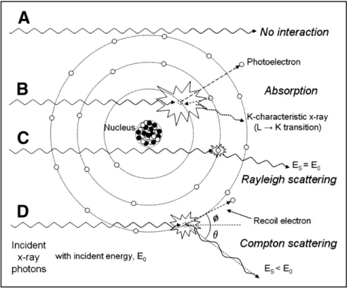
where theh is Planck’s constant. The photon interacts with matter while traveling through space, resulting in absorption and scattering of x-rays. The interaction between x-ray pho-ton and matter constitute the physics behind x-ray imaging. There are four main ways x-rays interact with matter: photoelectric absorption, Rayleigh scattering, Compton scat-tering, and pair production. The strength of these interactions are mainly determined by the x-ray photon energy and the material composition of the matter. For medical imaging, photoelectric absorption, Rayleigh scattering, and Compton scattering are most common interactions.(Figure 2.2)
2.2.1: Photoelectric Absorption
Figure 2.2: Illustration of x-ray and matter interactions. (A) Most x-ray photons have no interaction with the material, passing through unattenuated. (B) Photoelectric absorption results in total removal of the x-ray photon and production of a photoelectron, and a char-acteristic x-ray. (C) Elastic Rayleigh scattering with small change of trajectory of the x-ray photon. (D) Compton scattering between high energy photons and less bounded electrons. Scattering photon with less energy and a recoiled electron are generated.
[17]
electron or characteristic x-ray leads to another cascaded emission of characteristic x-rays or Auger electrons.
Figure 2.3: Illustration of photoelectric effect. (a) Photon absorption and ejection of photo-electron. (b) Characteristic x-ray emission.
[19]
Photoelectric absorption is subject to statistical processes. The probability of the effect is described by the cross section σ.[17]
σpe ∝ Zn
E3 (2.2)
2.2.2: Rayleigh Scattering
Besides being absorbed by matter, x-ray photons can be also scattered by atoms. Rayleigh scattering is one of the scattering interactions between x-ray photons and matter. It is an elastic scattering, meaning the energy of the scattered photon does not change, as shown in Figure 2.2. This process occurs when the incoming x-ray photon temporarily excites the electron without removing it from the atom, the excited electron returns to its normal energy state by emitting a photon with the same energy, but in a different direction. In this interaction, no energy is deposited into matter, thus it does not contribute to imaging dose. However, the scattered photons cause increased noise in the image which degrade image quality. Rayleigh scattering is more likely to happen with low energy x-ray photons and high Z material. The probability of Rayleigh scattering is described by the scattering cross-section:[17]
σR∝ Z2
E1.2 (2.3)
2.2.3: Compton Scattering
Compton scattering is another form of scattering between x-ray and matter. Compton scattering is an inelastic scattering. It is the dominant interaction for high energy x-ray photons. When the energy of the incident photon is much higher than the binding energy of the electron, part of the energy is transferred to the electron, which causes a recoil and removal of the electron. The remainder of the energy is transferred to the scattered photon, which has a trajectory with an angle of θ relative to the trajectory of the incident photon, as illustrated in Figure 2.2. θ is called the scattering angle. Both the total momentum and energy are conserved in this process, therefore, the scattered photon is given by:[17, 20]
Es =
Ei 1 + Ei
mec2(1−cosθ)
Where Es is the energy of the scattered photon, Ei is the energy of the incident photon, mec2 is the rest energy of electron (511keV), and θ is the scattering angle.
At low energies (∼ 5keV), x-ray photons are mostly back-scattered; at intermediate energy (∼ 20keV), the scattering photons are distributed approximately equally in all directions; while at high energies, the photons are forward scattered with a small scattering angle. [17] In x-ray imaging, these scattered photons can continue on to the x-ray detector, contributing to image noise and the degradation of the image contrast. Compton scattering also causes ionization in living tissue. As the incident photon energy increases, more energy is transferred to the the ejected electron, increasing the radiation dose to the object.
The cross-section of Compton scattering depends on the photon energies, when the x-ray energy between 10 keV and 100 keV, the cross-section is:[17]
σCLE ∝Z ·E0 (2.5)
while at the high energies (>100 keV), the cross-section is:[17]
σHEC ∝ Z
E (2.6)
2.2.4: Pair Production
Section 2.3: X-ray Attenuation
Due to the interactions of x-ray photons with matter discussed in the previous section, the combined effect is the attenuation of the x-rays, either through absorption or scattering, when x-rays pass through the material.
Consider a monochromatic x-ray beam, the attenuation of the beam intensity (I) was experimentally observed as:
dI
I =−µdx (2.7)
Where µis the constant for a given material and photon energy. The equation describes an exponential decay of the beam intensity. Given the incident beam intensity (I0), the exit beam intensity (I) after passing a material of thickness x is:
I =I0e−µx (2.8)
The µis called the attenuation coefficient, which statistically describes the probability of an x-ray photon interacting with matter. Like the individual ways of interaction, µis strongly dependent on incident photon energy and the density of the material. Generally, high Z materials have higher attenuation coefficients. The attenuation coefficient also decreases with increased photon energies.
Simply, if the object is composed by many materials, the beam intensity after attenuation is:
I =I0e
P
iµixi (2.9)
Section 2.4: Generation of X-ray
Section 2.2 briefly introduced the physical properties of x-ray, this section will focus on the generation of x-rays. X-ray, as a form electromagnetic radiation, is naturally generated through numerous physics processes, such as acceleration of charges, nuclear reactions, etc. Since the discovery of x-ray, scientists also found several ways to generate x-rays in laboratory settings. In this section, the mechanisms to produce x-rays will be briefly introduced.
2.4.1: Bremsstrahlung Radiation
Bremsstrahlung radiation occurs when one charged particle (usually electron) decelerates as it is passing by another charged particle (usually the nucleus of an atom). The energy of the photon equals the loss of the kinetic energy of the incoming charge. Thus the energy spectrum of Bremsstrahlung radiation is continuous, with the maximum possible energy equal to the kinetic energy of the incident charge. The maximum energy can only occur when all kinetic energy transfers to a single photon, in which case the probability is very small. Thus the number of photons decrease as photon energy increases.
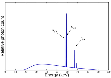
2.4.2: Characteristic X-rays
Figure 2.4: Illustration of the Bremsstrahlung radiation. An electron is deflected when passing by the nucleus of an atom, the loss of kinetic energy transfers to the x-ray photon.
lines. The Kα line is typically a doublet, with slightly different photon energy, due to the spin-orbit interaction energy between electron spin and orbit angular momentum. Kα lines are usually the strongest x-ray spectral line for an element. Figure 2.5 shows the energy spectrum of x-rays of a 90 kVp x-ray tube, with the characteristic lines marked.
2.4.3: Synchrotron Radiation
0 10 20 30 40 50 60 70 80 90 100
Energy (keV)
Relative photon count
Kβ 1 Kα 2 Kα 1
Figure 2.5: Energy spectrum of x-rays generated using a 90 kVp tube. The characteristic lines Kα1, Kα2, and Kβ1 are marked.
Section 2.5: X-ray Tubes
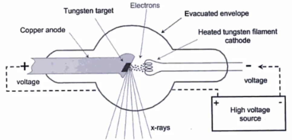
Currently, an x-ray tube is the most convenient way to generate x-rays controllably. The design of x-ray tubes haven’t changed significantly since William Coolidge invented the modern design of the x-ray tube in 1913 (Figure 2.7).[20]
Figure 2.7: Diagram of a Coolidge tube. The major component of the tube is the cathode, the anode, and the tube housing.
[20]
The x-ray tube consists of an electron source, and an anode target in a vacuum chamber. The anode is held at high voltage. Electrons emitted from the cathode are accelerated, and bombard the target material. Bremsstrahlung radiation is the main mechanism of x-ray production. If the anode voltage is high enough, characteristic radiation of the anode material is also generated.
2.5.1: Cathode
function of the metal, electrons are emitted from the cathode, which is called thermionic emission. In most modern tubes, a focusing cup electrode is placed behind the filament and at a negative voltage, propelling the emitted electrons to focus into a spot.
2.5.2: Anode
The anode in the x-ray tube is applied a positive high voltage.1 The electrons emitted from the cathode are accelerated by the electric field generated by the high anode voltage. The potential energy of the electric field is transferred to the kinetic energy of the electrons. The high speed electrons bombard the surface of the anode and penetrate into the target material. The electrons decelerate after hitting the anode, generating x-ray due to the Bremsstrahlung effect. If the electron energy is high enough, characteristic x-rays are also produced.
Over 99% of the energy of the electrons is transferred to heat. High atomic number targets yield to higher x-ray production efficiency. Therefore, high melting temperature and high atomic number materials are preferred for the anode. Tungsten, with a melting temperature of 3695 K and atomic number of 74, is the most commonly used anode material. When the electrons hit the anode surface, the penetration depth is on the order of a few hundred micrometers,[21] thus most heat is generated at the surface of the anode. To prevent anode cracking and pitting, an alloy of 10% rhenium (Re) and 90% tungsten is used to provide better resistance to surface damage.[20]
The anode heat load is a crucial issue to consider when designing the x-ray tube. For a low power tube, a stationary anode with highly conducting backing (typically copper) is used. However, to prevent anode damage, a rotating anode is often used in modern high power tubes. The rotating anode consists of the anode disk, the stem, and the rotor. Typical rotation speed of the anode is 3,000 RPM to 9,000 RPM.
2.5.3: Focal Spot
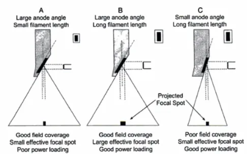
The electron trajectories are focused by the electric field. The area where electrons bombard the anode target is called the focal spot. The size of the focal spot is very import in x-ray imaging due to its direct involvement in the image resolution. Smaller focal spots yield to better spatial resolution.
For conventional x-ray tubes, the actual focal spot size depends on the size and shape of the filament. Since most filaments are long and thin, the focal spot is elongated in one direction, causing asymmetric spatial resolution in the image. To compensate for this, the anode and the detector are usually placed at an angle. This angle is referred as anode angle θ. The effective focal spot is the projected focal spot on the detector plane. The length of
the effective focal spot is the actual focal spot length times sinθ. The anode angle affects the field of view and the effective focal spot. Figure 2.8 illustrates this relationship. Generally, a small anode angle (∼ 7◦
−9◦) is desirable for small field of view applications, such as dental x-ray; while a larger anode angle (∼12◦
−15◦) is preferred for general radiographic applications.[20]
For most diagnostic imaging systems, the effective focal spot is isotropic, so that the image has the same spatial resolution along all directions. The (effective) focal spot size of an imaging system depends on the tradeoff between the imaging resolution requirement for the imaging task, the field of view, x-ray flux requirement, and anode heat load.
2.5.4: Tube Housing and Filtration
The cathode and anode are required to be placed in a vacuum environment to ensure the passing of electrons. The tube housing serves as a vacuum barrier. In addition, the housing also provides initial x-ray shielding, since the x-rays are produced in every direction. Dense materials, such as lead, are typically used for radiation shielding in the tube housing.
Figure 2.8: Illustration of the field of view and effective focal spot with respect to anode angle.
[20]
called the inherent filtration, since the window material also provides filtration to the x-ray spectrum. In addition to the inherent filtration of an x-ray tube, thin layers of material (typically aluminum) are also mounted outside the window for additional filtration of the beam. The filtration in an x-ray tube attenuates low energy photons to improve the beam quality. Since the low energy photons have little chance of passing through the patient in diagnostic imaging, filtering out this part of photons reduces the radiation dose to patient. The beam quality is quantitively measured by the half value layer (HVL) of the x-ray beam. HVL gives a measure of the effective energy of the beam. It is defined as the thickness of aluminum (in mm) required to reduce the intensity of the x-ray beam to half. The effective attenuation coefficient of aluminum µAlef f can be calculated from HVL:
µAlef f = ln 2
HV L (2.10)
Table 2.1: Excerpts of FDA HVL regulations for an x-ray tube operated between 60 kVp and 120 kVp.
X-ray Tube Voltage (kVp) Minimum HVL (mm of aluminum)
60 1.5
70 1.8
71 2.5
80 2.9
90 3.2
100 3.6
110 3.9
120 4.3
In the United States, the Food and Drug Administration (FDA) regulates the beam quality of x-ray for diagnostic imaging. All diagnostic imaging equipment must comply with the minimum HVL requirement specified in Title 21 of the Code of Federal Regulations.[22] Table 2.1 is an excerpt of HVL regulations for x-ray tubes between 60 kVp and 120 kVp.
Figure 2.9: Illustration of the effect of x-ray tube filtration on x-ray spectrum. (a) Shows the unfiltered Bremsstrahlung spectrum with great low-energy x-ray photon production. (b) Shows the filtered spectrum with preferential attenuation on the low energy photons.
[20]
CHAPTER 3: Digital Chest Tomosynthesis
Section 3.1: X-ray Imaging Modalities for Chest
There are three x-ray imaging modalities used in the clinic for chest examinations: chest x-ray radiography (CXR), computed tomography (CT), and digital chest tomosynthesis (DCT). This section will provide a brief introduction on each modality.
3.1.1: Chest X-ray Radiography
Chest x-ray radiography (CXR) is the most commonly practiced imaging procedure.[1] It is frequently the first imaging test performed on patients with known or suspected lung disease. It has been used for the diagnosis of diseases related to lungs and hearts such as infectious diseases, malignancies, airway diseases, interstitial diseases, bone diseases, and evaluation of trauma.
Different views of CXR can be obtained by changing the orientation of the chest and the direction of the incident x-ray beams. Posteroanterior (PA), anteroposterior (AP), and lateral views are the most common CXR views. The PA view is typically acquired with the patient standing up straight, in front of detector. The x-ray source is positioned behind the patient so that the x-ray beam can enter the posterior aspect (back) of the chest and exit from the anterior aspect (front) of the chest. In this exam, the source-to-image distance is typically 1.8 m.
determined using automatic exposure control (AEC).[3] The AEC chambers are embedded in the detector housing and are used to measured the radiation dose reaching the detector after passing through the patient. Once the reading from AEC reaches the designated value, it cuts off the x-ray output so that a reasonably good quality image is acquired at the lowest possible dose. For chest imaging, the AEC chambers are typically placed in the lung regions. Despite the low radiation dose, low cost, and high accessibility, there are several challenges for CXR. In CXR images, a 3D object is projected onto the 2D imaging plane. Organs and tissues along the path of x-ray beam are superimposed, resulting in loss of ”depth resolution”. Besides, the superposition of anatomical features may hide a lesion, leading to low sensitivity for the exams.
3.1.2: Computed Tomography
Until the invention of CT in 1972, x-ray imaging relied on 2D radiography. CT enables true 3D x-ray imaging. A CT scanner consists of an x-ray tube and a detector. But instead of fixing the positions of x-ray source and detector during image acquisition, both are mounted on a gantry and rotated around the object. The purpose of rotation is to allow x-rays to pass through all portions of the body through sufficient paths, so that the fully sampled object can be reconstructed using computers.
The principle of CT reconstruction is to calculate the attenuation coefficient of the material.[2] 3D datasets were calculated, and the value of each voxel is the CT number. The dataset is sliced along a certain direction and a stack of cross-sectional images are presented to the physicians.
CT results in high radiation dose to the patient. Studies have shown that the average dose of a two-view CXR is less than 1% of that of chest CT.[3]
However, due to cost, workflow, and radiation dose concerns, it is unlikely that CT will supplant CXR in the near future for general chest imaging. Therefore, an alternative low dose 3D imaging modality is desirable.
3.1.3: Digital Chest Tomosynthesis
DCT is an emerging low-dose tomographic imaging modality. It utilizes a small number of projection images acquired over a limited angle to produce quasi-3D image datasets. The technique yields some of the tomographic benefits of CT, but at lower cost and dose. It has been shown that the average dose of DCT is approximately 2% of chest CT.[3]
Section 3.2: Digital Tomosynthesis
3.2.1: Principles of Chest Tomosynthesis
The term ”tomosynthesis” was introduced by Grant in 1972.[24] It was combined from two Greek words: ”toms” – a section, a slice – and ”synthesis” – combining two or more pre-existing elements to get something completely new. Grant proposed a technique that uses a small number of projections to generate 3D images. However, it was not widely implemented until the development of digital detectors.
Current digital chest tomosynthesis (DCT) is illustrated in Figure 3.1. The system includes a conventional x-ray source, a computer controlled gantry that can be moved to various locations along a vertical path, a flat panel detector, and control electronics. The patient is positioned in front of a stationary detector, usually in PA position, as in CXR. Images are acquired and readout during the course of the tube movement.
Figure 3.1: Illustration of a DCT system. The system consists of a computer controlled gantry that can move the x-ray source to various locations long a vertical path, a flat panel detector, and computers.
[1]
image is the shift-and-add technique, as illustrated in Figure 3.2. The shift-and-add tech-nique is similar to the back projection techtech-nique in CT reconstruction. By shifting and adding the projection images, composite image slices at different planes are generated. Each plane is at a specific height. Only the object in the plane shows clearly in the reconstructed slice (Figure 3.2(B)). By scrolling through the reconstructed image set, different objects come in focus at different slices, while the object at other planes blurs out as artifacts.
Figure 3.2: Shift-and-add technique for tomosynthesis image reconstruction. In this illus-tration, five projection views are used for tomosynthesis reconstruction. The five images are shifted and added to yield composite images at two different planes. Different objects come in focus at different imaging planes.
[1]
3.2.2: Commercial DCT Systems
scan of 71 projections over a 20◦ angular span, within 11 s.[1, 8]
GE has developed a tomosynthesis option for their in-room digital radiography (DR) system. With the VolumeRAD option, the x-ray tube in the DR system can be moved in a vertical path to perform tomosynthesis with a variable source-to-detector distance of 180 cm -187 cm, as shown in Figure 3.3. A typical tomosynthesis scan takes 10 s and includes 61 low dose projections over 30◦.[10, 28] The tomosynthesis radiographic technique varies from patient to patient. The mAs per projection was determined using a scout view. [3, 27, 9]
Figure 3.3: Illustration and photo of GE VolumeRAD DCT system. [27]
Figure 3.4: Illustration of Shimadzu SONIALVISION DCT system. [13]
Table 3.1: List of key specs of the commercial DCT systems.
Commercial systems GE VolumeRAD Shimadzu Safire
Anode kVp 80 - 120 80 - 120
SID 180 - 187 cm (PA) 110 - 120 cm (AP) 110 - 130 cm (AP)
Number of projections 60 74
Angular coverage 30◦ - 35◦ 40◦
Scanning time 10 s 5 s
Focal spot size 0.6 mm/1.2 mm 0.4 mm
mAs per projection 1/6 of CXR N/A
3.2.3: Dosimetry of DCT Systems
DCT acquires low dose projection images to reconstruct tomosynthesis datasets. Cur-rently, most DCT uses the following protocol to determine the radiographic technique. When a patient is positioned, a scout view, which is a standard PA radiograph image using AEC, is acquired first. The technician uses this image to check the patient position and determine the technique for DCT acquisition. The mAs value from the scout view is multiplied by a constant, typically 10, and then divided by the total number of the projection views (61 for GE’s VolumeRAD system), to calculate the mAs setting for each projection.[3] For some of GE’s DCT system, the base DR system only has discrete settings for mAs. Thus the number is usually rounded down to the closest setting.[9]
In medical imaging, the effective dose is commonly used to measure the risk of radiation exposure. For standard chest CT, the effective dose is about 7 mSv.[3] For PA CXR, the average effective dose is around 0.017 mSv, while the two-view (PA + Lateral view) is 0.056 mSv.[3] Multiple studies have evaluated the effective dose for DCT. For adults, the average effective dose for a standard sized patient is approximately 0.1 mSv - 0.2 mSv.[3, 10, 13, 9]
3.2.4: Diagnostic Accuracy of DCT
Table 3.2: Comparison of CXR, DCT and CT for detection of lung nodules with CT as reference
3 - 5 (mm) 5 - 8 (mm) >10 (mm) Effective dose (mSv) [3, 9] Cost
CT 100% 100% 100% 2 - 7 High
CXR 7% [8] 19% [27] 63.6% [27], 53% [8] 0.02 - 0.06 Low
DCT 53% [8] 91.4% [27] 100% [27], 90% [8] 0.1 - 0.2 Medium
3.2.5: Limitations of Conventional DCT
CHAPTER 4: Carbon Nanotube X-ray Source
Section 4.1: Carbon Nanotube
Carbon nanotubes (CNTs) are allotropes of carbon with cylindrical crystal structure which was first discovered in 1991.[34] CNTs are members of the fullerene structure family. CNTs are long, hollow shaped tube structures with a high aspect ratio. Their walls are formed by graphene. Based on the number of layers, CNTs can be categorized as single-walled nanotubes (SWNTs) or multi-single-walled nanotubes (MWNTs). The diameters of SWNTs range from 0.4 nm to 2 nm, while those of MWNTs are between 2 nm to 100 nm. CNTs can be considered as graphene rolled at specific angles. The different ways of rolling result in a variance in properties of CNTs, such as metallic or semiconducting. [35]
CNTs can be synthesized using multiple techniques, such as arc discharge, laser ablation, chemical vapor deposition, etc.[36] Sumio Iijima synthesized the first CNTs using the arc discharge method in 1991.[34] Mass production of nanotubes is now available.[36]
Section 4.2: CNT Based Field Emission X-ray Source
4.2.1: Field Emission Effect
emission is described by the empirical formula:
J = (1−rav)A0T2e−
φ
kT (4.1)
Where rav is the reflection rate of outgoing electrons at the surface, T is the temperature of the filament, k is the Boltzmann constant, φ is the work function of the material, and A0 is a constant given by
A0 =
4πmk2e
h3 = 1.2×10
6Am−2K−2 (4.2)
The emission current increases as temperature rises. Using a material with high melting tem-perature, current density of conventional thermionic filaments can be up to 1000 mA/cm2.
In 1928, Ralph H. Fowler and Lothar Wolfgang Nordheim discovered the field emission effect.[37] Electrons are emitted by applying an external electric field to the material, instead of heating up the material, thus it’s also called ”cold electron emission”. The presence of the external electric field lowers the effective work function, so the electrons near the Fermi surface can tunnel through the potential barrier, as illustrated in Figure 4.1.[38] The emission current density is determined by the Fowler-Nordheim equation:[38]
J =aF 2 φ e
−bφF3/2
(4.3)
Whereaandbare constants with values of 1.54×10⁻⁶ A·eV·V−2 and 6.83eV−3/2·V ·nm−1, respectively. F is the applied electric field. The derivative of the current density
dJ dF ∝F e
−1
F (4.4)
Figure 4.1: Illustration of the field emission effect. The application of the electric field lowers the effective barrier so electrons near the Fermi level can tunnel through the barrier.
[39]
4.2.2: X-ray Source Using CNT Field Emitters
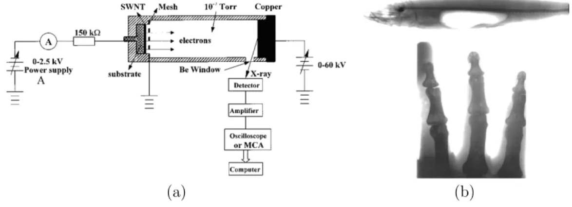
The high aspect ratio of CNTs makes CNTs excellent field emitters. Due to the sharp tip of CNTs, an enhanced field is created, which makes electrons easier to tunnel through the energy barrier.[40] CNTs have been studied as field emitters as early as 1995.[41] Early applications of CNT field emitters includes using CNT-based field emission displays,[42] and CNT as electron sources in x-ray tubes.[43]
to the power limit and vacuum conditions of this tube, the anode voltage was set to 14 kV.
(a) (b)
Figure 4.2: (a) Schematic of the triode-type field emission x-ray tube. (b) X-ray images of a fish and human hand phantom taken using the CNT x-ray source.
[44]