arXiv:1509.05768v3 [quant-ph] 20 May 2016
Arnau Sala1, 2,∗ and M. Blaauboer2,†
1
Lorentz Institute for Theoretical Physics, University of Leiden, 2333 CA Leiden, The Netherlands 2
Kavli Institute of Nanoscience, Delft University of Technology, Lorentzweg 1. 2628 CJ Delft, The Netherlands
(Dated: August 6, 2018)
We propose an implementation of a quantum router for microwave photons in a superconducting qubit architecture consisting of a transmon qubit, SQUIDs and a nonlinear capacitor. We model and analyze the dynamics of operation of the quantum switch using quantum Langevin equations in a scattering approach and compute the photon reflection and transmission probabilities. For parameters corresponding to up-to-date experimental devices we predict successful operation of the router with probabilities above 94%.
PACS numbers: 42.50.Ex, 85.25.Hv, 42.50.Pq, 03.67.Hk
INTRODUCTION
Given recent advances in experimental quantum com-putation, where few-qubit systems have been realized [1– 6], a considerable amount of research is currently devoted to investigating larger-scale systems such as networks for quantum communication [7–9]. In such systems, where information must be coherently transported over long distances, photons are suitable candidates as quantum in-formation carriers because of their long coherence times. Solid-state devices, on the other hand, seem preferable for storage of quantum information [10, 11]. Essential components in any quantum communication toolbox are, thus, devices capable of directing photons through differ-ent channels [8, 9, 12–14]. These devices include single-photon transistors [15–17], switches or routers [18–22], single-photon beam splitters [23,24], etc.
So far, several approaches have been proposed [25] for building a quantum switch, such as an optical implemen-tation using polarized photons and trapped atoms or a phase gate implementation [25]. Also, proposals for a beam splitter based on Superconducting Quantum Inter-ference Devices (SQUIDs) to route photons [23, 24,26– 28] or using toroidal resonators [29] have been put for-ward.
Here we propose a solid-state implementation of a quantum router using superconducting qubits. Given an n-photon input, consisting of a train of photon pulses where each of them can be in two states (or in a coherent superposition of both), the quantum switch absorbs the first photon and forwards the next n−1 photons to a path determined by the state of the first absorbed pho-ton. Our proposed device can be integrated in a larger network, where the output of one router is the input of the next. As a result, since the routers are controlled by the input signals there is no need to control the network externally. Also it requires the same number of photons to send a signal through two different paths with the same number of nodes, while other proposals [9,18] may require less photons for some preferred paths, leading to a network where some routes (e.g., a route that at each
bifurcation node takes the rightmost output path) have higher efficiency than others. We analyze the dynamic operation of the router using quantum Langevin equa-tions combined with input/output scattering formalism, taking into account decoherence due to relaxation and dephasing. We predict successful operation of the router with probabilities above 94% under realistic experimen-tal conditions.
The paper is organized as follows. First we present our proposal for the superconducting circuit that operates as a quantum router and derive the effective Hamiltonian of the system. We then analyze the dynamics of operation of the quantum switch using a scattering approach and calculate the probabilities of reflection and transmission of an incoming photon. In the last section conclusions and a discussion of the possible applications of this quantum device are presented.
MODEL
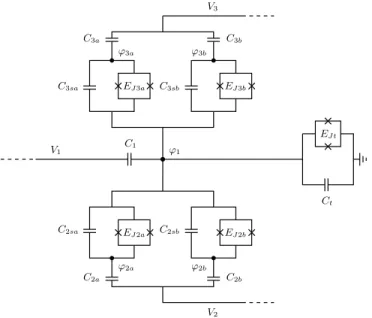
A schematic of the device we propose, based on circuit quantum electrodynamics (cQED), is depicted in FIG.1. The device is composed of three transmission lines capac-itively coupled to four SQUIDs and a transmon, acting as artificial atoms that absorb and reflect or transmit the photons forward. The device operates as follows: the first photon of a register that arrives at the switch is absorbed by the transmon which, after being excited, modifies the energy spectrum of the SQUIDs in such a way that the next photons can only be absorbed by the two SQUIDs labeled with 2aor 2b (3aor 3b) if the transmon is in its first (higher) excited state.
V1 C1 ϕ1
EJ t
Ct
C3sa EJ3a C3sb EJ3b
ϕ3a ϕ3b
C3a C3b
V3
V2 C2sa EJ2a C2sb EJ2b
ϕ2a ϕ2b
C2a C2b
FIG. 1. Circuit QED device proposed to operate as a quantum router. This device is composed of four SQUIDs, each with a capacitor (C2sa, C2sb, C3sa, C3sb) and a pair of
Joseph-son junctions (with energies EJ2a, etc.). It also contains a
transmon qubit, consisting of a capacitor (Ct) and a pair of
Josephson junctions (EJ t). These five elements are
capaci-tively coupled to an incoming transmission line (V1) and to
two outgoing transmission lines (V2 and V3). The fluxesϕi,
in the nodes of the circuit, are quantized variables (see [30] for the quantization of these variables) and describe the ab-sorption and emission of incoming photons by the transmon and SQUIDs.
of the register that controls the operation of the router, is prevented [30]. Also the coupling strength between the SQUIDs and their farthest transmission line is strongly reduced if this condition on the capacitances is satisfied. The dynamics of the router in FIG. 1 is described by an effective Hamiltonian [30]
Hef f =Hsys+Hc+HT. (1)
Here Hsys describes the energy levels of the transmon and SQUIDs and also the interaction between them:
Hsys= 3
X
i=1
ωT ia†T iaT i+
X
k
ωka†kak
−
3
X
i=1
X
k
Jika†T iaT ia†kak, (2)
with k∈ {2a,2b,3a,3b}. Here a† and adenote the cre-ation and annihilcre-ation operators for each of the energy levels of the system. These operators create an excitation with energyωT i in the transmon or ωk in the SQUIDs. The last term describes the density-density interaction between the i-th level of the transmon and the excita-tions in thek-th SQUID, with interaction strengthJik.
Hc describes the exchange interaction between the transmon and SQUIDs with the transmission lines, which are modeled as a bath of harmonic oscillators [31,32] with ladder operators b1, b2 and b3 for the first, second and third transmission lines, respectively:
Hc =
Z
dp
"
a†T1b1(p)
√πτ
T1 +a
† T3b1(p)
√πτ
T3
+
r 2
πτT1 −
r
3 πτT3
a†T2aT1b1(p)
+ a
† 2a
√πτ
a
+ a
† 2b
√πτ
b
!
(b1(p) +b2(p))
+ a
† 3a
√πτ
a + a†3b
√πτ
b
!
(b1(p) +b3(p)) +h.c.
#
.
(3)
The interaction strength of this coupling is given byτT1 andτT3, which are the lifetimes of the excited levels of the transmon, and alsoτa and τb, which are the lifetimes of the SQUIDs. Note that the transmon is only coupled to the incoming transmission line and that the second level of the transmon is not coupled (directly) to the trans-mission lines [33]. The coupling between the third level of the transmon and the transmission line —which is not present in the Jaynes-Cummings Hamiltonian, the ex-pression that usually describes cQED systems similar to FIG.1[2,4,34]— is achieved by introducing a nonlinear capacitor in the transmon [35] (see also Sup. Mat.). This nonlinear capacitor can be realized, e.g., by placing car-bon nanotubes between the plates of the capacitor [36]. These give rise to an energy spectrum that has the form E(V) = C2(V2+αV4) for small voltagesV[37, 38].
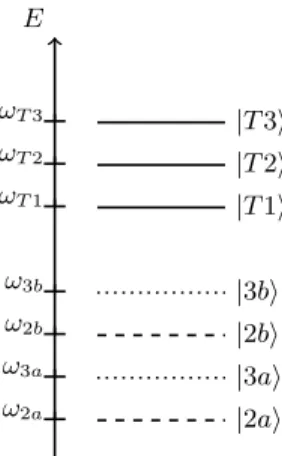
The energy spectrum of the device, described by the HamiltoniansHsys and Hc [Eq. (2) and (3)], is shown in FIG. 2. In this figure the three levels of the trans-mon are represented with solid lines. The energy levels of the SQUIDs, in dashed lines (coupled to the second transmission line) and dotted lines (coupled to the third transmission line), do not coincide since all the capaci-tances and Josephson energies are different. After send-ing a control photon —with energy ωT1 or ωT3— into the router (see Fig.3), due to the coupling between the transmon and SQUID energy levels described in Eq. (2), the energy needed to create an excitation in SQUID 2a when the first level in the transmon is occupied can be made equal to the energy needed to create an excita-tion in SQUID 3awhen the third level in the transmon is occupied (likewise for 2b and 3b). This can be done by tuning the energies of the Josephson junctions of the system. Thus, the transmon —the control element of the router— forwards a photon with energyωa (orωb) to the second or third transmission line, depending solely on the state of the control photon.
E
ω2a
ω3a
ω2b
ω3b
ωT1
ωT2
ωT3
|T1i
|T2i
|T3i
|2ai
|2bi
|3ai
|3bi
FIG. 2. Schematic representation of the energy spectrum of the Hamiltonian in Eq. (2). This spectrum only contains the ‘single-photon levels’, i.e., the levels that are accessible only by absorbing one single photon (plus|T2i, for completeness). Energy levels represented with solid lines are coupled only to the incoming transmission line. Dashed lines describe levels coupled to the second outgoing transmission line and also the incoming one. Dotted lines describe levels coupled to the third outgoing transmission line and also the incoming one. The separation of the energy levels is not to scale.
|T1i
|T1i |2ai
|T1i |2bi
|T1i |3ai
|T1i |3bi
ωa ωb
|T3i
|T3i |2ai
|T3i |2bi
|T3i |3ai
|T3i |3bi
ωa ωb
(a) (b)
FIG. 3. (Color online) Energy spectrum of the Hamiltonian in Eq. (2) after the transmon has been excited. (a) After the first energy level of the transmon has been excited, the next photon, which has energy either ωa orωb (or a
super-position of both) can only excite the energy levels coupled to the second outgoing transmission line. (b) If the third energy level of the transmon has been excited, the same photon can only excite the energy levels coupled to the third outgoing transmission line.
of oscillating modes as [31,32]:
HT =
Z
dp pb†1(p)b1(p) +b†2(p)b2(p) +b†3(p)b3(p).
(4)
ANALYSIS
In order to analyze the dynamics of the quantum router we have studied the scattering of one and two photons by our proposed device. Here we calculate the probabilities of reflection and transmission through each of the output channels.
We start by deriving the Langevin equations from the effective HamiltonianHef f [Eq. (1)] including relaxation and dephasing [30, 39]. We then obtain the equations of motion within the input/output formalism of quan-tum optics [16,32, 40]. From these equations we obtain the scattering amplitude of transmission and reflection of photons, assuming a Lorentzian pulse shape for the incoming photons [16].
Due to the multiple energy levels of the transmon (de-picted in FIG.2), the equation of motion for this element of the system —in terms of the operatorsa1anda†1 intro-duced after quantizing the fluxes [30]— is a complicated equation to work with. In order to simplify the calcu-lations we introduce three projection operatorsaT1,aT2 and aT3 and their hermitian conjugate —whose defini-tion can be found in the Supp. Mat.— to replacea1and a†1. Moreover, we have limited our Hilbert space by con-sidering only three excited energy levels in the transmon and only one in each of the SQUIDs. These operators, with the properties
a†T i|GSi= |T ii
a†T i|T ji=0 ∀i, j, (5)
and also
aT i|T ii= |GSi aT i|GSi= 0
aT i|T ji=0 ∀i6=j, (6)
with |GSibeing the ground state of the transmon and
|T iiits excited states, are projection operators that do not satisfy the usual commutation relations, so special care has to be taken when working with them. On the other hand, one of the advantages of using these three operators is that, although we will have three equations for the transmon instead of one, they are easier to solve. The use of these three operators instead of the original one does not change the model as long as the number of excited states of the transmon is limited to three. An-other advantage of using this notation is that the final quantized Hamiltonian takes a simpler form [the results being Eqns. (2) and (3)] and is easier to interpret: the operator describing the occupation of thei-th level of the transmon is simplya†T iaT i.
Before deriving the Langevin equations we must find an expression that describes the incoming and outgoing photons in the input/output formalism. Following [40] we introduce the operatorsb†2in andb
†
2out, and their her-mitian conjugates, which create an incoming and an out-going photon in the second transmission line (the same procedure must be applied to the other two transmission lines). These operators are defined as (see e.g. [16,40]):
b†2in/out(t) =√1
2π
Z ∞
−∞
whereωis the frequency of the photon andb2(ω, t1) is an initial (or final) value of the Heisenberg operator defined at a timet1→ −∞for the input operator (ort1→+∞
for the output operator). The Langevin equations of the ‘static’ variables of the system in terms ofb1in,b2in and b3in are shown in the Supp. Mat. Once the Langevin equations are found, relaxation and dephasing ratios are then introduced into this set of equations by following Refs. [39, 40].
Within the input/output formalism, the scattering am-plitude for a photon with frequencykin transmission line 1 to be reflected or transmitted in a transmission line i with frequencypis given by
S(p, k) =h0|bi,out(p)b†1in(k)|0i. (8)
In the case that multiple photons are sent in, the scat-tering amplitude reads
S(p1, . . . , pn;k1, . . . , kn) =
=h0|bi,out(p1). . . bi′,out(pn)b†1in(k1). . . b †
1in(kn)|0i. (9)
These scattering amplitudes are valid for incoming pho-tons with a definite frequencyk1, . . . , ki each or a super-position of these. Assuming that the incoming photons have a frequency distribution given by a Lorentzian cen-tered at ki = ωi and with width 1/τi, the scattering amplitude of a photon with frequencyω1is given by
β(p) =
Z dk1
√πτ1i(ω1 1 −k) + 1
τ1
S(p1, k1). (10)
The probability of this process to happen is given by:
P =
Z
dp|β(p)|2. (11)
Let us consider again the single photon processes. For a good performance of the quantum router, the first pho-ton to arrive must be absorbed by the transmon and be reflected back after all the other photons have been trans-mitted. It is, thus, necessary to find a procedure to find out whether the photon has been reflected after being absorbed or without being absorbed. For this purpose we describe the incoming photons as even modes given by the superposition of left and right-moving modes as b1in(k) = (r1in(k) +l1in(k))/
√
2 [32]. With this proce-dure one can see, after computing the scattering ampli-tudes and the probabilities, that a photon described as an even mode is absorbed (and reflected) with a large probability (see Tables I and II below). Moreover, the probability of transmission of subsequent photons is en-hanced if these are even modes.
The probabilities of reflection and transmission of pho-tons are obtained by numerically integrating the squared scattering amplitude over all momenta and imposing the
ωT1 ωT3 ω2a ωa
Refl. even modes 0.997 0.947 1.9·10−2
1 Refl. right-moving 0.998 0.973 0.238 1.6·10−5
Transmission 2 0 0 0.952 9.8·10−6
Transmission 3 0 0 1.6·10−6
2.3·10−6
TABLE I. Probabilities of reflection and transmission of an incoming photon. The probabilities in this table have been computed for different frequencies of the incoming photons and considering both even modes and right-moving modes. Similar values can be obtained for left-moving modes. The probability of reflection of a right-moving photon, as com-puted here, is equivalent to the probability of absorption plus reflection of the incoming photon.
conditionsω2a−J12a =ω3a−J33a =ωa and, similarly, ω2b−J12b=ω3b−J33b=ωa. This ensures that the router is controlled by the state of the first incoming photon.
The results of our calculations are shown in Tables I andII. The first table contains the probabilities of trans-mission of an incoming photon with different frequencies ωT1,ωT3,ω2aandωathrough the second and third trans-mission lines together with the probabilities of reflection in case this photon is described as an even mode or as a right-moving mode (see Sup. Mat. and [32] for a descrip-tion of these modes). In the case of a photon with energy ωT1or ωT3, since both energy levels are coupled only to the incoming transmission lines [see Eq. (3)], we find a large probability of reflection, above 94%. It is interest-ing to notice the different behavior of the router with respect to the form of the modes. In case the photons are described by even modes, the probability amplitude of reflection scales as
Seven∼ −
1−34γτT1 1 +34γτT1
(12)
for a photon with frequency ωT1. In this expression, γ is the rate of decoherence and τT1 is the lifetime of the excited energy level in the transmon. In case of right-moving modes, since a right-right-moving mode is reflected as a left-moving mode if it is absorbed and as a right-moving mode if it is reflected but not absorbed [16], the corresponding expression in TableIrepresents the prob-ability that a photon is absorbed and reflected, with an amplitude that is given by
Sright∼ − 1 1 + 34γτT1
. (13)
ω2a ωa ωb
Transmission 2 (T1) 4.45·10−6
0.952 0.964
Transmission 3 (T1) 7.58·10−5
1.63·10−6
1.47·10−6
Transmission 2 (T3) 2.43·10−7
7.12·10−7
2.94·10−6
Transmission 3 (T3) 4.45·10−6
0.952 0.964
TABLE II. Probabilities of reflection and transmission of a photon while one of the levels —T1 orT3— of the transmon is excited. Only even modes have been considered (see the text).
we are only interested in a scenario where the photons ab-sorbed by the SQUIDs are always transmitted, we only consider even modes from now on. Notice that the prob-ability of transmission of a photon indeed goes to one in case it is transmitted to the nearest transmission line of the excited SQUID (with even modes) and vanishes in case it is transmitted to the other outgoing transmission line.
More interesting is the case where two photons (a con-trol and a target photons) are sent into the router. In this case, while the transmon is in the (slow) process of absorption and emission of the control photon, the sec-ond (target) photon is absorbed and emitted in a faster process by a SQUID before the transmon returns to its ground state. The data corresponding to these scatter-ing processes is shown in TableII. In this case, a photon described by an even mode with energy eitherωa orωb is transmitted to the second transmission line with a prob-ability above 95% if the first level of the transmon is excited. The probability amplitude of transmission of a photon with energyωa to the second outgoing transmis-sion line is then given by
S2∼ 1
1 +3 8γτa
. (14)
If the third instead of the first level is excited, the photon is forwarded to the third outgoing transmission line with the same probabilities as in the case a photon is forwarded to the second transmission line when the first level of the transmon is excited. For any other frequency of the incoming photons these are not transmitted.
CONCLUSIONS AND OUTLOOK
We have proposed and analyzed a transmon-based quantum router containing a nonlinear capacitor that op-erates with photons in the microwave regime. The non-linear capacitor is the element responsible for the photon-transmon interaction. We predict successful operation of the quantum router with probabilities above 94% for cur-rent experimental parameters. That is, the probability
that a photon is transmitted successfully to the target channel, assuming that the transmon has been excited with a high probability (as the calculations suggest) and that the photon is transmitted before the transmon re-turns to its ground state, is above 94%. This router can be built with a set of capacitors and Josephson junctions (see Ref. [30] for a proposal of such parameters) in which two of the SQUIDs (coupled to the same outgoing trans-mission line) can be excited by a photon with frequency ωa or ωb if one (or the other) level of the transmon is excited.
The quantum router can be used as a single-photon transistor, with the distinctive characteristics that both the control and target photons can come from the same transmission line (i.e., from the same source) and that the target photon can be transmitted into two different transmission lines. The control photon thus not only controls whether the target photon is transmitted or not but also into which transmission line it is routed. Since the router is operated quantum-mechanically, this allows for transmission of photons in a superposition of paths if the control photon is in a superposition of states. Because of the latter, the proposed router can also be used to construct a quantum random access memory [41], where a tree-like network with quantum switches at the nodes leads an address register of qubits from the root node to a superposition of memory cells. Finally, the router could be used as a basic element in quantum communication networks. A list of requirements to fulfill this purpose is discussed in the Supplemental Material [30].
This work is part of the research programme of the Foundation for Fundamental Research on Matter (FOM), which is part of the Netherlands Organisation for Scien-tific Research (NWO).
∗ [email protected] † [email protected]
[1] H. H¨affner, C. Roos, and R. Blatt,
Physics Reports469, 155 (2008).
[2] L. DiCarlo, J. M. Chow, J. M. Gambetta, L. S. Bishop, B. R. Johnson, D. I. Schuster, J. Majer, A. Blais, L. Frunzio, S. M. Girvin, and R. J. Schoelkopf,
Nature460, 240 (2009).
[3] T. van der Sar, Z. H. Wang, M. S. Blok, H. Bernien, T. H. Taminiau, D. M. Toyli, D. A. Lidar, D. D. Awschalom, R. Hanson, and V. V. Dobrovitski,
Nature484, 82 (2012).
[4] E. Lucero, R. Barends, Y. Chen, J. Kelly, M. Mariantoni, A. Megrant, P. O’Malley, D. Sank, A. Vainsencher, J. Wenner, T. White, Y. Yin, A. N. Cleland, and J. M. Martinis,Nat. Phys.8, 719 (2012).
[5] C. Monroe and J. Kim,Science339, 1164 (2013).
[6] S. Barz, I. Kassal, M. Ringbauer, Y. O. Lipp, B. Daki´c, A. Aspuru-Guzik, and P. Walther,
Sci. Rep.4, 6115 (2014).
N. Gisin, L. Henzen, P. Junod, G. Litzistorf, P. Mon-baron, L. Monat, J.-B. Page, D. Perroud, G. Ribordy, A. Rochas, S. Robyr, J. Tavares, R. Thew, P. Trinkler, S. Ventura, R. Voirol, N. Walenta, and H. Zbinden,
New Journal of Physics13, 123001 (2011).
[8] S. Ritter, C. Nolleke, C. Hahn, A. Reiserer, A. Neuzner, M. Uphoff, M. Mucke, E. Figueroa, J. Bochmann, and G. Rempe,Nature484, 195 (2012).
[9] J. C. Garcia-Escartin and P. Chamorro-Posada,
Phys. Rev. A86, 032334 (2012).
[10] I. Chiorescu, N. Groll, S. Bertaina, T. Mori, and S. Miyashita,Phys. Rev. B82, 024413 (2010).
[11] H. Wu, R. E. George, J. H. Wesenberg, K. Mølmer, D. I. Schuster, R. J. Schoelkopf, K. M. Itoh, A. Ar-davan, J. J. L. Morton, and G. A. D. Briggs,
Phys. Rev. Lett.105, 140503 (2010).
[12] K. Lemr, K. Bartkiewicz, A. ˇCernoch, and J. Soubusta,
Phys. Rev. A87, 062333 (2013).
[13] K. Lemr and A. Cernoch,ˇ
Optics Communications300, 282 (2013).
[14] C.-C. Qu, L. Zhou, and Y.-B. Sheng,
International Journal of Theoretical Physics54, 3004 (2015).
[15] D. E. Chang, A. S. Sørensen, E. A. Demler, and M. D. Lukin,Nat Phys3, 807 (2007).
[16] L. Neumeier, M. Leib, and M. J. Hartmann,
Phys. Rev. Lett.111, 063601 (2013).
[17] M. T. Manzoni, F. Reiter, J. M. Taylor, and A. S. Sørensen,Phys. Rev. B89, 180502 (2014).
[18] I.-C. Hoi, C. M. Wilson, G. Johansson, T. Palomaki, B. Peropadre, and P. Delsing,
Phys. Rev. Lett.107, 073601 (2011).
[19] G. S. Agarwal and S. Huang,
Phys. Rev. A85, 021801 (2012).
[20] J.-J. Li and K.-D. Zhu,
Photonics and Nanostructures - Fundamentals and Applications10, 553 (2012).
[21] J. Lu, L. Zhou, L.-M. Kuang, and F. Nori,
Phys. Rev. A89, 013805 (2014).
[22] W.-B. Yan and H. Fan,Sci Rep4, 4820 (2014).
[23] L. Chirolli, G. Burkard, S. Kumar, and D. P. DiVin-cenzo,Phys. Rev. Lett.104, 230502 (2010).
[24] E. Hoffmann, F. Deppe, T. Niemczyk, T. Wirth, E. P. Menzel, G. Wild, H. Huebl, M. Mariantoni, T. Weißl, A. Lukashenko, A. P. Zhuravel, A. V. Ustinov, A. Marx, and R. Gross,Appl. Phys. Lett.97, 222508 (2010).
[25] See V. Giovannetti, S. Lloyd, and L. Maccone,
Phys. Rev. A78, 052310 (2008)and references therein.
[26] M. Mariantoni, F. Deppe, A. Marx, R. Gross, F. K. Wil-helm, and E. Solano,Phys. Rev. B78, 104508 (2008).
[27] C. M. Quintana, K. D. Petersson, L. W. McFaul, S. J. Srinivasan, A. A. Houck, and J. R. Petta,
Phys. Rev. Lett.110, 173603 (2013).
[28] T. H. Kyaw, S. Felicetti, G. Romero, E. Solano, and L.-C. Kwek,Sci. Rep.5, 8621 (2015).
[29] F. Hong, Y. Xiang, Z. Zhu, L. Jiang, and L. Wu,
Phys. Rev. A86, 010306 (2012).
[30] See Supplemental Material for derivations and additional analysys.
[31] M. H. Devoret, inQuantum Fluctuations ´Ecole d’´et´e de Physique des Houches Session LXIII, Les Houches, edited by S. Raimond, E. Giacobino, and J. Zinn-Justin (Else-vier, 1995) pp. 351 – 386.
[32] S. Fan, S¸. E. Kocaba¸s, and J.-T. Shen,
Phys. Rev. A82, 063821 (2010).
[33] Given that the Lagrangian of the system is an even
func-tion (see supp. material), only odd levels of the transmon and SQUIDs are coupled to the transmission lines.
[34] J. Koch, T. M. Yu, J. Gambetta, A. A. Houck, D. I. Schuster, J. Majer, A. Blais, M. H. Devoret, S. M. Girvin, and R. J. Schoelkopf,Phys. Rev. A76, 042319 (2007).
[35] Strictly speaking, after the addition of the nonlinear ca-pacitor the behavior of the transmon will be modified. This does not affect our calculations, however, since they involve the behavior of the system as a whole and not that of the transmon by itself. For simplicity, we refer to “transmons” and “SQUIDs” (and their energy levels) throughout the paper.
[36] S. Ilani, L. A. K. Donev, M. Kindermann, and P. L. McEuen,Nat. Phys.2, 687 (2006).
[37] Various systems give rise to nonlinear behavior of the ca-pacitance as a function of the potential [42–44], but only with carbon nanotubes the energy spectrum of the ca-pacitor has the formE(V) = C
2(V 2
+αV4
) [38] for small voltages V, which is required for obtaining the interac-tions in Eq. (3).
[38] D. Akinwande, Y. Nishi, and H.-S. Wong,
Nanotechnology, IEEE Transactions on8, 31 (2009).
[39] G. Ithier, E. Collin, P. Joyez, P. J. Meeson, D. Vion, D. Esteve, F. Chiarello, A. Shnir-man, Y. Makhlin, J. Schriefl, and G. Sch¨on,
Phys. Rev. B72, 134519 (2005).
[40] C. W. Gardiner and M. J. Collett,
Phys. Rev. A31, 3761 (1985).
[41] V. Giovannetti, S. Lloyd, and L. Maccone,
Phys. Rev. Lett.100, 160501 (2008).
[42] C. A.-P. de Araujo, J. D. Cuchiaro, L. D. McMillan, M. C. Scott, and J. F. Scott,Nature374, 627 (1995).
[43] E. Gluskin,International Journal of Electronics58, 63 (1985).
Proposal for a transmon-based quantum router: Supplemental Material
These notes contain some comments and additional information needed to understand the derivation of the results presented in the main text. We discuss in detail the need for a nonlinear capacitor in the proposed router design and possible candidates together with their properties. We also show how our model (Hamiltonian) has been derived and quantized and how scattering amplitudes and probabilities are computed. We present the set of numbers we have used and discuss obstacles and possible remedies towards scaling up of our proposed router. Finally, we discuss the requirements that we believe a quantum router needs to satisfy in order to construct a network for quantum communications.
NONLINEAR CAPACITORS
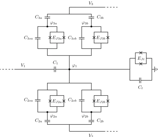
In circuit QED, a device similar to the one proposed in the main text (see also FIG. S4) is usually described by the Jaynes-Cummings (or Tavis-Cummings) Hamiltonian [1–3]. This Hamiltonian only allows the excitation of one level of the transmon by absorbing one photon. If the third level of the transmon is to be reached, then three photons are needed. Here we propose a mechanism with which the third level of the transmon can be excited in one step by absorbing one photon. Unfortunately this transmon-cavity interaction cannot be achieved by using Josephson junctions or any other inductive element (when including an inductive element in the Lagrangian and performing a Legendre transformation, the resulting Hamiltonian does not contain a term coupling the transmon with the transmission lines, as is required). The nonlinearity provided by a Josephson junction is insufficient to couple the third level of the transmon to the transmission lines in a way that allows for a photon to be absorbed by the system and drive the transmon from its ground state to its third excited state (|T3iin the main text). This photon-transmon interaction, not usually present in cQED devices, can, however, be achieved by using a nonlinear capacitative element. These capacitors have been realized and studied in multiple disciplines and with different implementations, such as using ferroelectric thin films or ceramics [4,5], quantum wells in heterojunctions [6], MOS junctions [7,8] and carbon nanotubes [9,10].
We are interested in a nonlinear capacitor whose energy is a non-quadratic, symmetric and increasing function of the voltage for small fluctuations ofV. In this way, the system will be confined into a region of small potentials [11]. Among the aforementioned nonlinear capacitors, the one based on carbon nanotubes seems to be the most suitable candidate. This capacitor [9] consists of two parallel plates with carbon nanotubes in between, placed perpendicular to the plates. The nonlinearity in the C(V) curve is due to the finiteness of the density of states (DOS) in the nanotubes [9, 10]. The capacitance of this device goes as C(V) ∼ C0(1 +αV2), thus the energy spectrum of this capacitor as a function of the potential difference across the plates has the form
E(V)∼
Z V
0
dV′(V −V′)C(V′) = 1 2C0(V
2+αV4), (S15)
where, to simplify the notation, the constantαhas been redefined to absorb a numerical constant.
Note that the carbon nanotubes do not constitute a key element in our proposal. Any other capacitative element, easier to fabricate and implement, with the same or similar energy spectrum will work as well.
THE MODEL: DERIVATION
given by
LS = C2a
2 ( ˙ϕ2a−V2) 2
+C2sa
2 ( ˙ϕ1−ϕ2˙ a) 2
+EJ2acos
ϕ1
−ϕ2a ϕ0
+C2b
2 ( ˙ϕ2b−V2) 2
+C2sb
2 ( ˙ϕ1−ϕ2˙ b) 2
+EJ2bcos
ϕ1
−ϕ2b ϕ0
+C3a
2 ( ˙ϕ3a−V3) 2
+C3sa
2 ( ˙ϕ1−ϕ3˙ a) 2
+EJ3acos
ϕ1
−ϕ3a ϕ0
+C3b
2 ( ˙ϕ3b−V3) 2
+C3sb
2 ( ˙ϕ1−ϕ3˙ b) 2
+EJ3bcos
ϕ1−ϕ3b ϕ0
, (S16)
where the dynamic variablesϕ1,ϕ2a,ϕ2b,ϕ3a andϕ3b are the fluxes defined at each node of the diagram in FIG.S4 andϕ0=~/(2e) is the flux quantum divided by 2π. For the transmon, the Lagrangian that describes its behavior is
given by
Lt= C1
2 ( ˙ϕt−V1) 2
+Ct 2 ϕ˙
2 t+αϕ˙41
+EJtcos
ϕ1
ϕ0
. (S17)
Note that the expression in Eq. (S17) contains the energy spectrum of a carbon nanotube nonlinear capacitor [right-hand side in Eq. (S15)].
The Legendre transformation of the Lagrangian in Eq. (S16) and (S17), needed to study the quantum dynamics of the router, gives a function that is not easy to work with due to the presence of quadratic and cubic radicals. Instead, a Taylor expansion of the transformation is more suitable for our purposes. The expanded Hamiltonian is given by:
H =p 2
2a+ 2p2ac2aV2−C2saC2aV22 2(C2a+C2sa)
+p 2
2b+ 2p2bc2bV2−C2sbC2bV22 2(C2b+C2sb)
+p 2
3a+ 2p3ac3aV3−C3saC3aV32 2(C3a+C3sa)
+p 2
3b+ 2p3bc3bV3−C3sbC3bV32 2(C3b+C3sb)
+x 2
2γ − βx4 12γ4 +
β2x6 18γ7 −
β3x8 18γ10 −
C1V2 1
2 −EJtcos
ϕ1
ϕ0
−EJ2acos
ϕ1
−ϕ2a ϕ0
−EJ2bcos
ϕ1
−ϕ2b ϕ0
−EJ3acos
ϕ1−ϕ3a ϕ0
−EJ3bcos
ϕ1−ϕ3b ϕ0
. (S18)
For the sake of simplicity, the Hamiltonian in Eq. (S18) is expressed in terms of the fluxes, their conjugate momenta and the variablex, defined as
x≡p1+C1V1+ C2sa
C2a+C2sa(p2a+C2aV2) +
C2sb
C2b+C2sb(p2b+C2bV2)
+ C3sa
C3a+C3sa(p3a+C3aV3) +
C3sb
C3b+C3sb(p3b+C3bV3), (S19)
with
β≡6Ctα (S20)
γ≡C1+Ct+ C2aC2sa C2a+C2sa
+ C2bC2sb C2b+C2sb
+ C3aC3sa C3a+C3sa
+ C3bC3sb C3b+C3sb
. (S21)
In order to give rise to a density-density interaction between the different energy levels, the Hamiltonian is required to contain a term withp6
1p22a (see the next section in which the Hamiltonian is quantized). This expression appears after expanding the Hamiltonian in a Taylor series. In this same expansion a term containing p3
1V1 appears which describes the coupling between the third energy level of the transmon and the transmission lines.
V1
C1
ϕ1
EJ t
Ct C3sa EJ3a C3sb EJ3b
ϕ3a ϕ3b
C3a C3b
V3
V2
C2sa EJ C2sb
2a EJ2b
ϕ2a ϕ2b
C2a C2b
FIG. S4. Circuit QED device proposed to operate as a quantum router. This device is composed of four SQUIDs, each with a capacitor (C2sa, C2sb, C3sa, C3sb) and a pair of Josephson junctions (with energiesEJ2a, etc.). It also contains a transmon
qubit, with a capacitor (Ct) and a pair of Josephson junctions (EJ t). These five elements are capacitively coupled to an
incoming transmission line (V1) and to two outgoing transmission lines (V2andV3). The fluxesϕi, in the nodes of the circuit,
are quantized variables (see the text around the figure, sectionThe model: derivation, for the quantization of these variables) and describe the absorption and emission of incoming photons by the transmon and SQUIDs. In this proposal, two SQUIDs are placed in each branch for scalability purposes and robustness. Since the target photons can be in two states with different frequencies (for scaling purposes, for these will be the control photons in a subsequent router), two resonators (per branch) coupled to the same transmission line, with two distinct threshold energies for which they are detuned, are needed to absorb the target photons.
Quantization of the Hamiltonian
The Hamiltonian is quantized as usual by introducing the ladder operators as follows:
p1=− i~
2ϕ0
3
2 γ2 βET
1/4
(a1−a†1) (S22)
φ1=
2
3 βET
γ2
1/4
(a1+a†1). (S23)
Here we have made use of the variableφ1=ϕ1/ϕ0, to simplify the derivations, where ϕ0 = ~
2e and also ET =
~2
8γϕ2 0.
The operatorsa1anda†1are the usual ladder operators that annihilate and create an excitation in the transmon. For the SQUIDs, the quantized forms of the operators are
p2a=− i~
2ϕ0
"
EJ2a
C2a+C2sa C2sa
β
6γ2E T
1/2#1/2
(a2a−a†2a) (S24)
φ2a=
"
1 EJ2a
C2sa C2a+C2sa
6γ2E T β
1/2#1/2
Similar expressions can be derived for the other operators. With Eqns. (S22) – (S25) together withEJt+EJ2a + EJ2b+EJ3a+EJ3b = 3γ2/β ≡E¯J and EJ2aE2a = ( ¯EJ−EJ2a+EJ2b+EJ3a+EJ3b) (for simplicity we have also introducedE2a =
~2
8C2saϕ 2
0) the SQUID-transmon exchange interactions are strongly suppressed and the expressions
describing the energy levels of the system together with the density-density interactions between them are found [see Eq. (2) in the main text]. The SQUID-SQUID exchange interaction can be neglected since its interaction strength goes as (C2sa/C2a)2. Other similar interactions can be neglected by making the capacitances C2sa, C2sb, C3sa and C3sbsmaller than all the others and using the rotating wave approximation.
The interaction Hamiltonian [Eq. (3) in the main text], which couples the transmon and the SQUIDs with the incoming and outgoing transmission lines, is derived by imposing the following quantization of the potentialsV1, V2 andV3:
Vi=− i~
2ϕ0A 1/4
i (bi−b†i). (S26)
Here bi, b†i are the ladder operators describing the oscillating modes in thei-th transmission line, and Ai are three constants that may be different.
Let us look again the expressions in Eqns. (S18) and (S19). In the Hamiltonian [Eq. (S18)], there are only even powers ofx. If we consider a single incoming photon, contained inV1 [see Eq. (S26)], given that the terms in the Hamiltonian containing a single power of V1 only contains odd powers of the momenta, the photon will excite only odd levels of the system. An even level can only be excited if an odd level is already occupied. This is shown in the HamiltonianHc in the main text [Eq. (3)].
Projection operators
In order to simpliby both the notation and the calculations we have introduced three projection operators defined as
a†T1≡16a21a†1 3
=
0 0 0 0 0 0 0 0 0 0 0 1 0 0 0 0
, (S27)
a†T2≡ 1
3√2a1a † 1 3
=
0 0 0 0 0 0 0 1 0 0 0 0 0 0 0 0
, (S28)
a†T3≡√1
6a † 1 3
=
0 0 0 1 0 0 0 0 0 0 0 0 0 0 0 0
, (S29)
to replacea1and its hermitian conjugate. The Hamiltonian in the main text is written in terms of these new operators (see the sectionAnalysis). These operators have the property that a†T i acting on the ground state of the transmon creates an excitation in thei-th level, whereas the same operator acting on any other state where the transmon is already excited gives zero. Similarly, the operatoraT ionly annihilates an excitation of levels in the transmon, lowering it to its ground state.
With these projection operators, the quantized Hamiltonian Hc, which describes the coupling between the trans-mission lines with the transmon and SQUIDs takes the simple form
Hc =
Z
dp
"
a†T1b1(p)
√πτ
T1 +
a†T3b1(p)
√πτ
T3 +
r
2 πτT1 −
r
3 πτT3
a†T2aT1b1(p) +
r
3 πτT1 −3
r
2 πτT3
a†T3aT2b1(p)
+ a
† 2a
√πτ
a
+ a
† 2b
√πτ
b
!
(b1(p) +b2(p))) + a † 3a
√πτ
a
+ a
† 3b
√πτ
b
!
(b1(p) +b3(p))) +h.c.
#
The fourth term in the right-hand side, whose hermitian conjugate describes the process where the third excited level of the transmon decays into the second while emitting a photon, can be canceled by settingαas
α= γ 3ϕ2
0
324~Ct. (S31)
In this way, the number of states the third level of the transmon can evolve into is reduced and, thus, the lifetime of the third level of the transmon is enhanced, increasing the transition matrix element from the ground state to|T3i.
Langevin equations of motion
The Langevin equations of the ‘static’ variables of the system in terms ofb1in,b2inandb3in are
˙ aT1=−
iωT1+ 1 τT1
aT1− 1
√τ
T1τT3 aT3+i
X
k
J1kaT1a†kak+ 2
r 2
τT1 −
r
3 τT3
a†
T1aT2
√τ
T1 +a
† T3aT2
√τ T3 ! + 1 √τ T1
a†T1aT1−aT1a†T1
+√1 τT3
a†T3aT1 a2a
√τ
a +√a2b
τb +√a3a
τa +√a3b
τb
+
r 2
τT1−
r
3 τT3
a† 2a √τ a + a † 2b √τ b + a † 3a √τ a + a † 3b √τ b !
aT2
+i
r 2
τT1
a†T1aT1−aT1a†T1
+
r
2 τT3a
† T3aT1
b1in(t)−i
√
2
r 2
τT1 −
r
3 τT3
b†1in(t)aT2, (S32)
˙ aT3=−
iωT3+ 1 τT3
aT3− 1
√τ
T1τT3 aT1+i
X
k
J3kaT3a†kak
+
1
√τ
T1
a†T1aT3+ 1
√τ
T3
a†T3aT3−aT3a†T3
a2a
√τ
a +√a2b
τb +√a3a
τa +√a3b
τb
+i
r
2 τT1
a†T1aT3+
r
2 τT3
a†T3aT3−aT3a†T3
b1in(t), (S33)
˙ a2a =−
iω2a+ 2 τa
a2a+i 3
X
j=1
Jj2aa†T jaT ja2a−i
r
2 τa
(b1in(t) +b2in(t))
−√2a2τ b
aτb − a3a
τa − a3b
√τ
aτb − 1
√τ
a
r
2 τT1 −
r
3 τT3
a†T1aT2−√ 1 τaτT1
aT1−√ 1 τaτT3
aT3, (S34)
where the index k in the sum runs over k ∈ {2a,2b,3a,3b} and three more equations for 2b, 3a and 3b, similar to Eq. (S34), have to be derived. Relaxation and dephasing ratios are then introduced into this set of Langevin equations by following Refs. [14,16].
PHOTON MODES IN THE TRANSMISSION LINES
In this section we briefly describe the meaning of the left/right-moving and even/odd modes, which are common in many circuit-QED works where the input-output formalism is used. For more details we refer the reader to Ref. [17], appendix A, where the following description is taken from.
In case the photons in a transmission line are allowed to propagate in both directions, the photon modes are described by right-moving bosonic operators (r,r†) if they propagate to the right or by left-moving bosonic operators (l,l†) if they propagate to the left. In this case, the Hamiltonian that describes the transmission lines reads:
HT =
Z ∞
−∞ dp p r†
prp−l†plp
, (S35)
Ct C2a C2b C3a C3b C2sa C2sb C3sa C3sb
0.1C1 1.2C1 1.1C1 C1 C1 0.1824C1 0.1934C1 0.1560C1 0.1799C1
TABLE S3. Proposal for a set of parameters that satisfy the requirements of a quantum router, given in terms of the capacitance
C1 = 10−
9e2
~F. With these values, the device can operate as described in the main text, forwarding photons into one of the outgoing transmission lines according to the state of the control photon. The rest of the parameters (Josephson energies, inductances,α) are found as functions of the capacitances during the derivation of the quantized Hamiltonian (see the second section of these supplementary notes) .
in this case, contain the sum of operatorsr+landr†+l†instead ofbandb† for each transmission line, so the different components of the router interact equally with both the left and right-moving modes.
From this new Hamiltonian, and following the same procedure as before (input/output formalism), similar equations of motion are found. Nevertheless, we can also do one more step and define two new operators: the even (b,b†) and odd (˚b, ˚b†) operators that describe what are called even and odd modes, defined as:
bp=
rp+l−p
√
2 , (S36)
˚bp=rp−l−p
√
2 . (S37)
These we then introduce in the Hamiltonian replacing the right and left-moving modes. One can check that the odd modes are not coupled to the system (they do not appear in the interacting part of the Hamiltonian), so they can be omitted in the Hamiltonian. The even modes are the ones used in the main text.
NUMERICAL INTEGRATION OF THE SCATTERING AMPLITUDES
In order to find the set of values for the capacitances —these are the only free parameters left— that best satisfy the requirements for an optimal quantum router it is convenient to maximize (or minimize) the scattering probabilities according to the operating requirements. Since an analytical solution has proved difficult to obtain, we have looked, by trial and error, for a set of numbers with which the router works as expected and found a set of capacitances that satisfy our requirements of energy spacing between the SQUIDs and transmon levels. Then, by maximizing the scattering amplitudes we have fine-tuned these values. Although a more systematic way of searching may result in a better solution, we have found that there exist at least one set of such parameters, shown in Table S3. The reason for this fine tuning is that, although the separation between the energy levels of the transmon is relatively large, the separation between the energy levels of the SQUIDs is very small (and the optimal operation of the quantum router sensitively depends on small variations of the values of the capacitances)
With the values in TableS3, the energies are found to be around 10GHz for the transmon energy levels (ωT1 = 7.189GHz and ωT3 = 21.93GHz ) and around 1GHz for the SQUIDs (ω2a = 1.028GHz, ω2b = 1.162GHz, ω3a = 1.053GHz and ω3b = 1.186GHz). The coupling strength is of the order of 10−7Hz. All these values are common in the related literature. Also, we used the ratio ¯EJ/ET = 1296 which, although being larger than in other circuit-QED works, is sufficient to give rise to the nonlinear effects needed for the correct operation of the quantum router [3].
For the two-photon processes, we have made some assumptions: from the single-photon process, we have seen that the transmon absorbs the first incoming photon with a large probability, so for the two-photon processes we assumed that we sent the second photon while the transmon is already excited and that it does not decay emitting the control photon until the second photon has been fully transmitted. This implies that the lifetime of the transmon is much larger than that of the SQUIDs. This is a plausible assumption, given that the lifetimes of such cQED devices depend not only on the elements they are composed of but also on the geometry of the system (Purcell effect, see e.g. [18]).
magnitude larger than that of the SQUIDs with the current set of capacitances. A possible solution may be to add a device between the two consecutive routers that enlarges the energy of the first photon to arrive. Stimulated Raman Adiabatic Passage (STIRAP) processes may be a candidate for a device capable of transferring the population of one quantum state (with lower energy) to another (with higher energy). These processes have been studied in circuit QED systems in [19,20].
REQUIREMENTS FOR AN EFFICIENT QUANTUM ROUTER FOR QUANTUM COMMUNICATIONS
So far, different proposals for quantum switches or routers that may be implemented in a quantum network have been studied [21–25]. In order to assess the suitability of a given implementation for efficient use in a quantum communication network, we list here a set of requirements that we believe a quantum router must satisfy (part of these have been proposed elsewhere [24,25]). The list below contains general requirements, which can be applied and checked for specific implementations.
Imagine we have a network for quantum communication composed of quantum channels (which allow for the transmission of quantum information) and nodes (which contain quantum routers). Consider also that there is a signal to be sent and an element that controls the switches.
1.The information in the signal to be transmitted and also the information encoded in the control elements must be stored in quantum objects (qubits). Otherwise we can not talk about a fully quantum-mechanical router [24].
2.The router has to be able to route the (quantum) signal into a coherent superposition of both output modes [24].
3.The signal information must remain undisturbed during the entire routing process [24]. The control information must also remain undisturbed, so that we can keep track of the signal and verify that it is not modified (due to e.g., entanglement with the control element).
4.The router has to work without any need for postselection on the signal output [24].
5.To optimize the resources of the quantum network, only a single control qubit is required to direct each signal qubit [24]. Alternatively, the control information could also be stored in the signal qubit itself [25], but that may give the receiver information about the network which, in some applications, may not be a good idea.
6.With one single control qubit, as many as possible signal qubits should be forwarded.
7.A router withnoutputs must operate with the same efficiency (or speed, or with the same number of operations, etc.) for each output channel.
8.Scalability: the output of a router should be the input of the next one in a network.
The quantum router that we propose satisfies all of these requirements except for the last one (although, as we discussed in the previous section, this problem can for example be amended by using STIRAP processes). We thus believe that it can become a good candidate for a quantum switch or router in a network for quantum communication.
∗ [email protected] † [email protected]
[1] L. DiCarlo, J. M. Chow, J. M. Gambetta, L. S. Bishop, B. R. Johnson, D. I. Schuster, J. Majer, A. Blais, L. Frunzio, S. M. Girvin, and R. J. Schoelkopf,Nature460, 240 (2009).
[2] E. Lucero, R. Barends, Y. Chen, J. Kelly, M. Mariantoni, A. Megrant, P. O’Malley, D. Sank, A. Vainsencher, J. Wenner, T. White, Y. Yin, A. N. Cleland, and J. M. Martinis,Nat. Phys.8, 719 (2012).
[3] J. Koch, T. M. Yu, J. Gambetta, A. A. Houck, D. I. Schuster, J. Majer, A. Blais, M. H. Devoret, S. M. Girvin, and R. J. Schoelkopf,Phys. Rev. A76, 042319 (2007).
[4] C. A.-P. de Araujo, J. D. Cuchiaro, L. D. McMillan, M. C. Scott, and J. F. Scott,Nature374, 627 (1995).
[5] E. Gluskin,International Journal of Electronics58, 63 (1985).
[6] N. Sengouga, R. Boumaraf, R. H. Mari, A. Meftah, D. Jameel, N. A. Saqri, M. Azziz, D. Taylor, and M. Henini,
Materials Science in Semiconductor Processing36, 156 (2015).
[7] J. Colinge and C. Colinge, Physics of Semiconductor Devices(Springer, 2002).
[9] S. Ilani, L. A. K. Donev, M. Kindermann, and P. L. McEuen,Nat. Phys.2, 687 (2006).
[10] D. Akinwande, Y. Nishi, and H.-S. Wong,Nanotechnology, IEEE Transactions on8, 31 (2009).
[11] If the energy is a function of the potential across the two plates of the capacitor whose minimum is not at V = 0, a perturbation of the system will drive it to a region in the potential space of larger voltages, but in this region the analysis we make is not valid anymore because the dynamic variables that we quantize are small fluctuations of the potentials.
[12] L. S. Bishop,Circuit Quantum Electrodynamics,Ph.D. thesis, Yale University (2010).
[13] M. H. Devoret, inQuantum Fluctuations ´Ecole d’´et´e de Physique des Houches Session LXIII, Les Houches, edited by S. Raimond, E. Giacobino, and J. Zinn-Justin (Elsevier, 1995) pp. 351 – 386.
[14] C. W. Gardiner and M. J. Collett,Phys. Rev. A31, 3761 (1985).
[15] L. Neumeier, M. Leib, and M. J. Hartmann,Phys. Rev. Lett.111, 063601 (2013).
[16] G. Ithier, E. Collin, P. Joyez, P. J. Meeson, D. Vion, D. Esteve, F. Chiarello, A. Shnirman, Y. Makhlin, J. Schriefl, and G. Sch¨on,Phys. Rev. B72, 134519 (2005).
[17] S. Fan, S¸. E. Kocaba¸s, and J.-T. Shen,Phys. Rev. A82, 063821 (2010).
[18] M. D. Reed, L. DiCarlo, S. E. Nigg, L. Sun, L. Frunzio, S. M. Girvin, and R. J. Schoelkopf,Nature482, 382 (2012).
[19] J. Siewert, T. Brandes, and G. Falci,Optics Communications264, 435 (2006).
[20] Z.-B. Feng, Z.-L. Cai, C. Zhang, L. Fan, and T. Feng,Optics Communications283, 1975 (2010).
[21] G. S. Agarwal and S. Huang,Phys. Rev. A85, 021801 (2012).
[22] I.-C. Hoi, C. M. Wilson, G. Johansson, T. Palomaki, B. Peropadre, and P. Delsing,Phys. Rev. Lett. 107, 073601 (2011).
[23] J. Lu, L. Zhou, L.-M. Kuang, and F. Nori,Phys. Rev. A89, 013805 (2014).
[24] K. Lemr, K. Bartkiewicz, A. ˇCernoch, and J. Soubusta,Phys. Rev. A87, 062333 (2013).