REGISTRATION AND ANALYSIS OF DEVELOPMENTAL IMAGE SEQUENCES
Istvan Csapo
A dissertation submitted to the faculty of the University of North Carolina at Chapel Hill in partial fulfillment of the requirements for the degree of Doctor of Philosophy in the
Department of Computer Science.
Chapel Hill 2018
Approved by:
Marc Niethammer
Martin Styner
Eva Anton
ABSTRACT
Istvan Csapo: Registration and Analysis of Developmental Image Sequences (Under the direction of Marc Niethammer)
Mapping images into the same anatomical coordinate system via image registration is a fundamental step when studying physiological processes, such as brain development. Standard registration methods are applicable when biological structures are mapped to the same anatomy and their appearance remains constant across the images or changes spatially uniformly. However, image sequences of animal or human development often do not follow these assumptions, and thus standard registration methods are unsuited for their analysis.
In response, this dissertation tackles the problems of i) registering developmental image sequences with spatially non-uniform appearance change and ii) reconstructing a coherent 3D volume from serially sectioned images with non-matching anatomies between the sections.
ACKNOWLEDGEMENTS
First and foremost, I thank my advisor, Marc Niethammer, for his support and unwavering enthusi-asm. Marc is a generous mentor and a first-rate teacher. I am grateful for having had the opportunity to work with him.
I thank my committee, Martin Styner, Eva Anton, Alex Berg, and Vladimir Jojic for their support and valuable feedback. My collaborators at the Neuro Image Research and Analysis Laboratories, Martin Styner and Yundi Shi, contributed heavily to the work presented in the first part of this dissertation.
It has been a great pleasure to work with the members of the Anton Lab and the associated staff at the Department of Cell Biology and Physiology. I am especially thankful to Eva Anton for sharing his deep knowledge of brain development and giving me the opportunity to work on such a fundamentally important problem; to Martis Cowles for the excellent discussions and close collaboration on the neuron migration project; to Gary Wilkins for spending countless hours behind the microscope to collect our images and teaching me the surgical and lab skills used to prepare the samples; and to Vladimir Ghukasyan for improving our images and teaching me how to use the confocal microscope.
I thank my fellow lab mates, Tian Cao, Heather Couture, Yi Hong, Liang Shan, and Xiao Yang—I drew a lot of inspiration from their work. I thank the faculty and staff members of the Department of Computer Science who were always willing to help.
TABLE OF CONTENTS
LIST OF TABLES . . . viii
LIST OF FIGURES . . . ix
LIST OF ABBREVIATIONS . . . xii
1 Introduction . . . 1
1.1 Motivation . . . 1
1.1.1 Temporally-Dependent Image Similarity Measure . . . 3
1.1.2 Registration of Developmental Image Sequences with Missing Data . . . 3
1.1.3 3D Reconstruction of Serially Sectioned Images . . . 4
1.2 Thesis and Contributions . . . 5
1.3 Overview of Chapters . . . 6
2 Background . . . 7
2.1 Image Registration . . . 7
2.1.1 Similarity Measures . . . 9
2.1.2 Regularization . . . 10
3 Temporally-Dependent Image Similarity Measure . . . 12
3.1 Model-Based Similarity Measure . . . 14
3.1.1 General Local Intensity Model Estimation for SSD . . . 14
3.1.2 Logistic Intensity Model with Elastic Deformation . . . 15
3.2 Parameter Estimation . . . 16
3.2.1 Registration Model . . . 16
3.3 Experimental Results . . . 17
3.3.1 White Matter Intensity Distributions from Real Data . . . 19
3.3.2 Experiment 1: Model Selection . . . 20
3.3.3 Experiment 2: Synthetic Data . . . 23
3.3.3.1 Affine transformation model . . . 24
3.3.3.2 Deformable registration . . . 25
3.3.4 Experiment 3: Simulated Brain Data . . . 25
3.3.4.1 Smoothing kernel size . . . 28
3.3.4.2 White matter segmentation . . . 28
3.3.5 Experiment 4: Monkey Data . . . 29
3.4 Conclusions. . . 32
4 Quantitative MRI Atlas of Postnatal Rhesus Macaque Brain Maturation . . . 34
4.1 Introduction. . . 34
4.2 Estimating the Atlas from a Population . . . 36
4.2.1 Monkey Dataset . . . 37
4.2.2 Model Estimation . . . 38
4.2.3 Comparison to Expected Myelination Pattern . . . 39
4.3 Conclusions. . . 41
5 Registration of Developmental Image Sequences with Missing Data . . . 42
5.1 Using the Maturation Information . . . 43
5.2 Experimental Results . . . 43
5.2.1 Registering Synthetic 2D Dataset . . . 44
5.2.2 Registering Real 3D Dataset . . . 46
5.2.2.1 Accuracy of affine registration . . . 46
5.2.2.2 Influence of prior with missing data . . . 50
5.3 Conclusions. . . 51
6.0.1 Previous Work . . . 56
6.1 Image Acquisition . . . 58
6.1.1 Measuring Tissue Loss Due to Sectioning . . . 59
6.2 3D Reconstruction . . . 62
6.2.1 Manual Preprocessing . . . 65
6.2.2 Intensity Normalization . . . 67
6.2.3 Segmentation . . . 67
6.2.4 Stacking . . . 69
6.2.5 Reconstruction . . . 70
6.3 Experimental Results . . . 71
6.3.1 Reconstructing 3D Synthetic Data . . . 72
6.3.1.1 Experiment . . . 72
6.3.2 Reconstructing Confocal Microscopy Embryonic Mouse Data . . . 74
6.3.3 Mapping Neuron Migration in the Developing Brain . . . 76
6.4 Conclusions. . . 80
7 Discussion . . . 84
7.1 Summary of Contributions . . . 84
7.2 Future Work . . . 87
7.2.1 Model-Based Similarity Measure . . . 87
7.2.2 Atlas of Brain Maturation . . . 87
7.2.3 Template-free 3D Reconstruction . . . 88
LIST OF TABLES
3.1 Model selection experiment results . . . 23
3.2 Landmark registration error . . . 31
5.1 Registration error for synthetic data experiment with varying prior weights . . . 45
5.2 Registration error for monkey data experiment . . . 51
LIST OF FIGURES
1.1 Mouse embryo development: 9.5-12.5 days . . . 2
2.1 Registration overview . . . 7
2.2 Standard similarity measures . . . 10
3.1 Simplified model of neurodevelopment . . . 12
3.2 Logistic intensity model . . . 15
3.3 Synthetic dataset with logistic white matter intensity change and longitudinal deformation over time . . . 18
3.4 Simulated brain images . . . 19
3.5 Spatiotemporal distribution of white matter intensities in 9 monkeys . . . 20
3.6 Synthetic datasets with 10 time points generated with various intensity models . . . 21
3.7 The influence of the intensity model on the registration . . . 22
3.8 Experimental setup for synthetic datasets . . . 24
3.9 Experiment 1: results with affine transformation . . . 26
3.10 Experiment 1: results with deformable transformation . . . 27
3.11 The effect of various smoothing kernel sizes on the intensity model estimation . . . 29
3.12 SSR registration: effect of smoothing kernel size . . . 30
3.13 SSR registration: effect of white matter segmentation accuracy . . . 30
3.14 Corresponding target and source landmarks for a single subject . . . 31
3.15 Experimental setup and results for a single subject . . . 32
3.16 Landmark distance mismatch . . . 33
4.1 Axial slices of MR brain images of monkey at ages 2 weeks, 3, 6, 12, and 18 months . . . . 35
4.2 Example of an expert-defined anatomical landmark . . . 37
4.3 Intensity model . . . 39
5.1 Synthetic dataset with logistic white matter intensity change . . . 44
5.2 Registration results with no prior . . . 46
5.3 Subset of landmarks . . . 47
5.4 Cartoon depiction of the typical anterior-posterior deformation . . . 49
5.5 Landmark errors per time point . . . 49
5.6 Registration results for a single subject . . . 52
6.1 Neurogenesis and differentiation . . . 54
6.2 Mouse embryo development . . . 58
6.3 Serial sectioning of the embryonic mouse brain . . . 59
6.4 Microscopy imaging of tissue sections . . . 61
6.5 Tissue loss of confocal microscopy sections . . . 63
6.6 Synthetic serially-sectioned dataset . . . 64
6.7 Serially-sectioned mouse embryo dataset . . . 65
6.8 Optical slices from a tissue section . . . 66
6.9 Evaluation of the tissue mask . . . 67
6.10 Intensity normalization of tissue sections . . . 68
6.11 Serially-sectioned dataset tissue masks . . . 69
6.12 3D reconstruction algorithm . . . 71
6.13 3D synthetic dataset: reconstruction example . . . 73
6.14 3D synthetic dataset: reconstruction results . . . 74
6.15 3D synthetic dataset: reconstruction errors . . . 75
6.16 Mouse dataset reconstruction results: axial view . . . 75
6.17 Mouse dataset reconstruction results: E14 . . . 76
6.18 Mouse dataset reconstruction results: E16 . . . 77
6.19 Mouse dataset reconstruction results: E18 . . . 78
6.20 Mouse dataset reconstruction results: FAS . . . 78
6.22 3D reconstruction results . . . 81
6.23 3D neuron migration atlas . . . 82
LIST OF ABBREVIATIONS
CT Computed Tomography
MI Mutual Information MR Magnetic Resonance
CHAPTER 1 Introduction
1.1 Motivation
With the advancement of biological imaging technologies, living organisms can be studied at an ever increasing spatial and temporal resolution. Various imaging modalities provide measurements at scales ranging from the molecular mechanisms of individual cells to the structural organization of whole organ systems. The latest microscopy and genetic techniques have allowed researchers to continuously capture and track thousands of cells during the development of the fruit fly embryo (Amat and Keller,2013) and image the complete real-time neuronal activity of the zebrafish (Keller and Ahrens,2015). These advances in biological imaging technologies, coupled with advances in genetics (Deisseroth,2015) and biochemistry (Chung and Deisseroth,2013), enabled researchers to probe and study complex biological processes in unprecedented detail.
One of the most complex biological processes is animal development. In the earliest stages of embryonic development, a single cell is transformed into thousands of cells that are organized into tissues and further grouped into organs and organ systems to form a fully functional organism. In later stages, neural circuitry is established in the central nervous system and neurons form a dense network of synaptic, electric, and modulatory connections from which function and complex behaviors arise. Normal function is dependent on the proper structural organization of cells at various scales, and disruptions to the orderly organization of cells can have severe detrimental effects on the developed organism. In humans, disruptions during the development of the central nervous system can lead to impairment that continues through adult life and may cause a wide variety of disorders, including autism spectrum disorders and schizophrenia (Bailey,1998;Bill and Geschwind,2009;Evsyukova et al.,2013).
Figure 1.1: Mouse embryo development from embryonic age 9.5 days to 12.5 days [Image from: Dr. Erica D. Watson, University of Cambridge (with permission)].
stages of the mouse embryo shown in Figure1.1. The first three images span only 24 hours and a single confocal fluorescence microscopy acquisition of one of the embryonic brains (a dataset analyzed in a later chapter), that is no larger than2mm3, can generate5×109 voxels with high enough resolution to show individual neuronal axons.
The nonlinear nature of the appearance and shape change of anatomical structures during development pose a significant challenge for accurate analysis. Many of the existing methods to analyze and quantify biological imaging data rely on assumptions of similarities in structure and appearance between individual images that no longer hold for these highly dynamic datasets. New image analysis methods are required to model complex developmental processes and to uncover subtle deviations from normal development while being able to deal with the large structural and appearance changes present in the image sequences. One of the fundamental image analysis steps is mapping images into the same coordinate system. For biological datasets, this coordinate system is commonly in anatomical space and the mapping is established via image registration. There are two primary approaches for establishing the mapping between images. The first uses common features, such as edges or segmented structures, in the images to find corresponding points. The second approach, used in this dissertation, is based on the intensity values of the images directly without extracting any geometric features.
the anatomically equivalent structures in the images that do not hold for many datasets acquired during development.
This dissertation focuses on registration methods for biological image sequences acquired during development. There are three primary contributions. The first contribution is a model-based similarity measure for longitudinal image registration in the presence of spatially non-uniform appearance change over time. The second contribution is a method for registering longitudinal datasets with missing time points, using an appearance atlas built from a population. The third contribution is a template-free registration method to reconstruct images of serially-sectioned biological samples into a coherent 3D volume.
1.1.1 Temporally-Dependent Image Similarity Measure
Certain biological processes are best studied by acquiring in-vivo longitudinal image sequences of the organism. One such process is brain development. The resulting time-varying datasets often capture not only the considerable morphological changes, but also appearance changes. Mapping such image sequences into the same anatomical coordinate system is challenging since standard similarity measures rely on strong assumptions about the appearance of anatomical structures that no longer hold in this case. These similarity measures are too restrictive to account for the appearance change of the same anatomical structures and instead induce deformations—that result in incorrect mapping between images—to achieve similarity.
In order to facilitate the correct mapping between anatomical structures that go through appearance change, I present a novel similarity metric that incorporates a time-dependent appearance model into the registration framework. The model is used to change the appearance of the target image to match the moving image. Then the moving image can be registered to the intensity-adjusted target image, effectively removing the appearance change for a good model.
1.1.2 Registration of Developmental Image Sequences with Missing Data
some acquisitions are corrupted and the resulting dataset is incomplete. While an improvement over the standard similarity measures, the temporally-dependent similarity measure I present is fully data-driven and parameter estimation may, therefore, become unreliable if the number of images in the longitudinal dataset is low. Furthermore, estimation of the model parameters is not possible if the number of available images is lower than the number of unknowns in the parametric intensity model.
One approach to account for missing time points during the parameter estimation step is to include prior knowledge about the model parameters into the model. For the temporally-dependent similarity measure, I incorporate a population maturation atlas as a prior to better guide the deformable registration for longitudinal datasets with missing time points. The prior is weighted such that its influence diminishes as the number of available time points increases. The atlas is built from a population of rhesus macaque monkeys with complete longitudinal datasets, and the proposed method is evaluated on datasets with missing time points.
1.1.3 3D Reconstruction of Serially Sectioned Images
While longitudinal studies are powerful for studying certain biological processes over time, there are several tradeoffs compared to cross-sectional studies. In cross-sectional studies subjects are not imaged multiple times, but rather a section of the population is imaged once. This type of study design is practical since the images can be collected in a short period of time by choosing subjects that span the whole extent of the biological process of interest. For example, in order to study the effects of aging on the normal human brain, a cross-sectional study can collect data from young and old subjects at the same time instead of having to follow subjects for decades.
Another advantage of cross-sectional studies is ability to use destructive imaging techniques. For longitudinal studies, the organism has to remain intact and thus only in-vivo imaging techniques can be used. For studying brain development, this excludes high resolution microscopy techniques that usually require tissue staining and sectioning—although, this has been changing as new technologies such as light sheet (Keller and Ahrens,2015) microscopy have enabled the high resolution in-vivo imaging of small organisms.
into a coherent 3D volume that resembles the geometry of the intact sample before sectioning. Existing reconstruction methods either require an imaging modality with dense structural information or using an external template as a reference image volume that is not available for many studies. I present a novel method for reconstructing serially-sectioned fluorescence microscopy images without an external template. These images also lack the dense structural information needed by many commonly used reconstruction methods.
1.2 Thesis and Contributions
Thesis: Advanced image registration methods can allow accurate anatomical mapping between images that are dissimilar in appearance or anatomy. Such registration methods are essential for analyzing
animal brain development.
The following contributions are presented in this dissertation:
1. A temporally-dependent similarity measure to aid the registration of longitudinal datasets with appearance change over time.
2. A developmental atlas of the neonatal rhesus macaque brain that captures the appearance change of the maturing white matter in a population of normal subjects.
3. A longitudinal registration method that can use a population atlas to deal with missing time points in a longitudinal image sequence.
1.3 Overview of Chapters
The remaining chapters are organized as follows:
Chapter 2 provides an overview of the topics that are discussed in this dissertation, including background on image registration focusing on similarity metrics and regularization.
Chapter3introduces a novel temporally-dependent similarity measure for longitudinal registration. The method is validated on two longitudinal datasets: a synthetic phantom image dataset and a real dataset of magnetic resonance images of the macaque brain, with manually selected landmarks for validation.
Chapter4presents a population atlas capturing the appearance changes over time of the macaque monkey during early postnatal development. The atlas is built from the parameters of the model-based similarity measure introduced in the previous chapter.
Chapter5presents a registration method, based on the temporally-dependent similarity measure, for longitudinal datasets with missing time points. The population atlas built in the previous chapter is used as a prior for this registration method.
Chapter6 presents a novel approach for reconstructing images acquired from serially-sectioned biological samples into a coherent 3D volume, without relying on an external template.
CHAPTER 2 Background
2.1 Image Registration
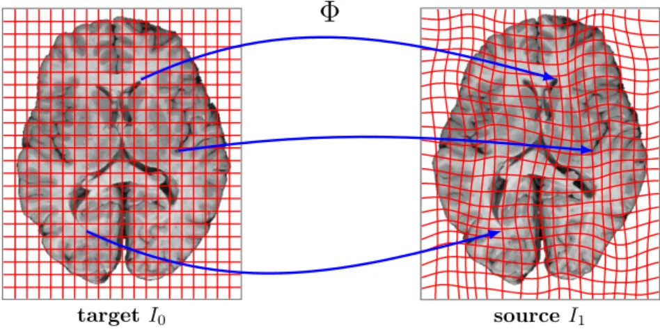
Finding correspondences between images is one of the fundamental problems of image analysis. Correspondence between images establishes a common coordinate system that is meaningful within the context of the image analysis problem. In medical image analysis, for example, the common coordinate system is often in anatomical space that allows mapping between structurally or functionally similar regions. Figure2.1shows the mapping between two brain images. Corresponding brain structures have a similar appearance in both images, hence an appearance based registration method can find the mapping between them. Registration can be performed between two or more images, but in this section I focus on registration problems involving two images. One image is usually referred to as the source (or moving) image and the other as the target (or fixed) image.
target I0 source I1
Φ
Figure 2.1: Spatial correspondence of two brain images. The space transformationΦmaps the coordinates of the target image to the corresponding anatomical coordinates of the source image. The aim of image registration is to recoverΦ.
features between the images, or direct measures of image intensity differences (such as sum of squared difference, cross correlation, or mutual information). In medical image analysis, finding manually defined landmarks is prohibitively time consuming and most images lack reliable dense features; therefore, image intensity based measures are the most commonly used similarity measures. It is important to note that images are assumed to have similar structure and appearance for typical image registration methods. However, this assumption does not always hold for biological images of development, where not only the morphology but the appearance of the observed organisms or structures can change drastically over time as well.
The aim of image registration is to recover the transformation that maps the images into the same coordinate system, while simultaneously restricting the transformation to the space of feasible trans-formations. Feasibility, again, depends on the application, but typically the aim is to avoid folding or tearing in the deformed images. When registering bone, for example, we might want to allow only rigid transformations, but allow deformable transformations for soft tissue registration. One way to enforce feasible transformations and at the same time make the overall estimation problem well-posed is either by restricting the deformation model to parametric models (such as similarity, rigid, or affine) or, for non-parametric deformation models, by imposing regularity on the deformation field.
Formulating image registration as an optimization problem, we want to find a transformationΦthat minimizes the joint objective function
E=S[Φ] | {z }
regularizer
+ 1
σ2D[I0, I1◦Φ− 1]
| {z }
similarity term
, (2.1)
whereSis the regularization term that encouragesΦto be a plausible (usually smooth) transformation,
Dis the image similarity measure,I1◦Φ−1is the transformed source image, andσcontrols the tradeoff
2.1.1 Similarity Measures
The role of the similarity term is to measure the quality of the alignment. The global optimum of the measure, therefore, should signal perfect alignment between the images. Three of the commonly used similarity measures are the sum of squared differences (SSD), normalized cross correlation (NCC), and mutual information (MI).
SSD assumes the image intensities to be identical at corresponding spatial locations (I0 =I1). This assumption is not valid for multimodal images or images with a change in appearance. It is the most specific similarity measure of the three and defined as
SSD[I0, I1] = Z
Ω
(I0(x)−I1(x))2dx,
whereΩis the image domain.
Normalized cross correlation is based on a weaker assumption of only an affine intensity relationship (I0 =aI1+b):
N CC[I0, I1] = 1 kI0kkI1k
Z
Ω
I0(x)I1(x)dx,
wherekIik= p
hIi, Iiiandh·,·iis the inner product.
Mutual information (MI) (Viola and Wells, 1995; Collignon et al., 1995) assumes a statistical relationship between the images without making any assumptions about the nature of this relationship. Therefore, it is suitable for a wide range of registration problems and it is the most general measure used for comparison in this thesis. The idea is to maximize the mutual information between two images with respect to the transformation. This is achieved by calculating the joint histogram, expressing the joint probabilities over the whole image. MI is defined as
M I[I0, I1] =H(I0) +H(I1)−H(I0, I1),
whereH(·)is the marginal andH(·,·)is the joint entropy. The joint entropy is calculated from the joint probability density,ρ(i0, i1), of the images as
H(I0, I1) =− X
i0,i1
wherei0andi1are the possible image intensities forI0andI1. In practice, the joint density is calculated from the joint image histogram and in that casei0 andi1 represent intensity ranges corresponding to the histogram bins. The marginal entropies are calculated similarly from the marginal densities. MI is maximum when the mapping between the intensities (or intensity ranges)i0 andi1 produces “sharp” joint histogram.
Figure 2.2: The graph on the left shows the optimal intensity relationships between two imagesI0andI1 with intensitiesi0andi1, respectively, for SSD (red), NCC (green), and MI (blue).∆i0and∆i1are the histogram bin widths used for MI. Note that for MI the intensity ranges do not need to lie on a line. The graph on the right is the joint histogram of two synthetic images (gray matter is the thin outer layer, white matter is the inner gray region)I1andI0(perfectly aligned) with either uniform white matter or with a spatial white matter intensity gradient. In the presence of the gradient the optimal intensity relationship is not satisfied for any of the measures, and therefore they will induce registration errors.
2.1.2 Regularization
In this dissertation, I use the elastic regularizer for the deformable registration experiments. It is based on the physical model of linear elasticity and it is defined on the displacement fielduas
S[u] = Z
Ω
µ
4 d X
j,k=1
(∂xjuk+∂xkuj)
2
| {z }
rigidity
+ λ
2(divu) 2
| {z }
volume change
dx,
CHAPTER 3
Temporally-Dependent Image Similarity Measure
The effect of appearance change on the result of image registration depends on the chosen trans-formation model and the chosen image similarity measure. Generally, transtrans-formation models with few degrees of freedom (such as rigid or affine transformations) are affected less by local changes in image appearance than transformation models which can capture localized spatial changes, such as elastic or fluid models. As later shown in Section3.3.3, affine methods perform well even in the presence of strong non-uniform appearance change, while deformable methods introduce erroneous local deformations in order to resolve inconsistencies in appearance. However, transformation models which can capture local deformations are desirable for many longitudinal studies as changes in morphology tend to be spatially non-uniform.
+
+
+
+
=
=
=
=
in
tensit
y
deformation
image
age
For longitudinal registration, temporal regularization of the transformation model has been explored recently. This is motivated by the assumption that unrealistic local changes can be avoided by enforcing temporal smoothness of a transformation (Durrleman et al.,2009;Fishbaugh et al.,2011). In this chapter, I instead focus on the complementary problem of determining an appropriate image similarity measure for longitudinal registration in the presence of temporal changes in image intensity.
Approaches which address non-uniform intensity changes have mainly addressed registration for image-pairs. These approaches either rely on local image uniformities (Loeckx et al.,2010;Studholme et al.,2006) or try to estimate image appearance changes jointly with an image transform (Friston et al., 1995;Roche et al.,2000;Miller and Younes,2001;Periaswamy and Farid,2003). Often (e.g., for bias field compensation in magnetic resonance imaging), image intensity changes are assumed to be smooth in both space and time. This assumption is not valid for certain applications, including longitudinal magnetic resonance (MR) imaging studies of neurodevelopment.
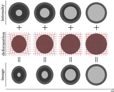
The changes seen on the MR images during neurodevelopment result from a variety of concurrent biological processes. Changes in various factors of tissue composition, such as myelin and water content, are coupled with both tissue generation and tissue loss (Casey et al.,2005). The majority of the changes seen in MR images, however, can be attributed to the myelination of the neuronal axons and morphological changes due to growth. In a simplified model of neurodevelopment, these two processes can be decoupled and modeled separately as shown in Figure3.1. The goal is to register the images in the bottom row. Existing deformable registration algorithms can resolve the morphological differences between source and target images if the image intensities within tissue classes remain constant or vary slowly. Therefore, if the model of intensity change is known the intensity change can be modded out and the only remaining task of the registration method is to recover the spatial transformation (middle row), reducing the original problem to registering each source image in the bottom row to the corresponding intensity adjusted target image in the top row.
maturation, the proposed method is general and can be applied to any longitudinal image registration problem with non-uniform appearance change (for example, time-series imaging of contrast agent injection).
Section3.1introduces the model-based image similarity measure, sum of squared residuals (SSR). Section 3.2 discusses parameter estimation. Section 3.3 describes the performed experiments and discusses results.
The work presented in this chapter has been published in (Csapo et al.,2012b,a,2013).
3.1 Model-Based Similarity Measure
Assume we have an image intensity modelIˆ(x, t;p)which for a parameterization,p, describes the expected intensity values for a given pointxat a timet. This model is defined in a spatially fixed target image,IT. Then, instead of registering a measured imageIiatti to a fixed target imageIT, we can register it to the corresponding intensity-adjusted target imageIˆ(x, ti;p), effectively removing temporal intensity changes for a good model and a good parameterization,p. Hence,
Sim(Ii◦Φ−1i , IT) is replaced by Sim(Ii◦Φ−1i ,Iˆ(x, ti;p)),
where Sim(·,·)is any chosen similarity measure (e.g., sum of squared differences (SSD), normalized
cross correlation, or mutual information), andΦ−i 1 is the map from imageIi to the spatially fixed target space. Since the proposed method aims to create an intensity adjusted modelIˆthat matches the appearance of the source image, SSD is an appropriate choice for the similarity measure. The new intensity-adjusted SSD similarity measure becomes the sum of squared residual (SSR) model, where the residual is defined as the difference between the predicted and the measured intensity value.
3.1.1 General Local Intensity Model Estimation for SSD
Since SSR is a local image similarity measure, for a given set ofN measurement images{Ii}at times{ti}we can write the full longitudinal similarity measure as the sum over the individual SSRs, i.e.,
SSR({Ii};p) = N−1
X
i=0 Z
Ω
whereΩis the image domain of the fixed image. For given spatial transformsΦi, Equation (3.1) is simply a least-squares parameter estimation problem given the measurements{Ii◦Φ−i 1(x)}and the predicted model values{Iˆ(x, ti;p)}. The objective is to minimize Equation (3.1) while, at the same time, estimating the model parametersp. The optimum is found by alternating optimization with respect to the intensity model parameters,p, and the spatial transformationsΦito convergence (see Section3.2). Note that looking at only two images at a time without enforcing some form of temporal continuity would lead to independent registration problems and discontinuous temporal intensity models. However, this potential problem is avoided by using all available images in the longitudinal set to estimate the intensity model parameters.
3.1.2 Logistic Intensity Model with Elastic Deformation
t i
2w 3m 6m 12m 18m
α
Figure 3.2: Logistic intensity model. SSR can be combined with any model for
in-tensity change, ranging from a given constant tar-get image (the trivial model) and linear models to nonlinear models that are more closely adapted to the myelination process during neurodevelopment. Since the myelination process exhibits a rapid in-crease in MR intensity (in T1 weighted images) dur-ing early brain development followed by a gradual
leveling off (Dobbing and Sands,1973), nonlinear appearance models are justified. I use a logistic model for the experiments, which is often used in growth studies (Fekedulegn et al.,1999), but also investigate various polynomial models in Section3.3.2. The logistic model is defined as
ˆ
I(x, t;α(x), β(x), k(x)) = α(x)
1 +β(x)e−k(x)t , (3.2)
white matter intensities. This is a simplifying, but reasonable, assumption since intensity inhomogeneities in unmyelinated or myelinated white matter are small compared to the white matter intensity change due to the myelination process itself (Barkovich et al.,1988).
3.2 Parameter Estimation
Once the parameters for the local intensity models are known, SSR can be used to replace the image similarity measure in any longitudinal registration method. Here, I use an elastic deformation model (Section3.2.1) and jointly estimate the parameters for the intensity model (Section3.2.2).
3.2.1 Registration Model
The growth process of the brain not only includes appearance change but complex morphological changes as well, hence the need for a deformable transformation model. To single out plausible deformations, I use an elastic regularizer (Broit,1981) defined on the displacement fielduas
S[u] = Z Ω µ 4 d X j,k=1
(∂xjuk+∂xkuj)
2
| {z }
rigidity
+ λ
2(divu) 2
| {z }
volume change
dx,
whereµ(=1) andλ(=0) are the Lamé constants that control elastic behavior and the div is the divergence operator defined as∇ ·u, where∇is the gradient operator. The behavior of the elastic regularizer might be better understood if we convert the Lamé constants to Poisson’s ratioν(=0) and Young’s modulusE
(=2). The given Poisson’s ratio allows volume change such that the change in length in one dimension does not cause expansion or contraction in the other dimensions. This is a desirable property in our case, since tissue is both generated and destroyed during development resulting in volume change over time. Young’s modulus, on the other hand, describes the elasticity of the tissue and was chosen experimentally to allow large deformations while limiting the amount of folding and discontinuities.
3.2.2 Model Parameter Estimation
The intensity model parameters are only estimated within the white matter where image appearance changes non-uniformly over time; for simplicity, gray matter intensity was assumed to stay constant. The methods for obtaining the white matter segmentations for each dataset are described in the corresponding experimental sections. In addition, the effect of white matter segmentation accuracy on the model-based registration is investigated in Section3.3.4.2.
Instead of estimating the parameters independently for each voxel, spatial regularization was achieved by estimating the medians of the parameters from overlapping local3×3×3neighborhoods (the effect of various neighborhood sizes on registration accuracy is investigated in Section3.3.4.1).
The algorithm is defined as follows:
0) Initialize modelIˆparameters top=p0(constant intensity model if no prior is given).
1) Affinely pre-register images{Ii}to {Iˆ(ti)}.
2) Estimate model parameterspfrom the pre-registered images.
3) Estimate the appearance ofIˆat times {ti}, giving {Iˆ(ti)}.
4) Estimate displacement fields{ui}by registering images{Ii}to{Iˆ(ti)}.
5) Estimatepfrom the registered images{Ii◦ui}.
6) Repeat from step 3 until convergence.
The algorithm terminates once the registration energy decreases by less than a given tolerance between subsequent iterations. In the experiments only a few iterations (typically less than 5) were required. If desired, a prior model defined in the target image (a form of intensity model parameter atlas) could easily be integrated into this framework.
3.3 Experimental Results
• Synthetic 2D (Figure3.3)
• Simulated brain images 3D (Figure3.4)
• Real monkey data 3D (Figure3.14)
For the synthetic and simulated datasets, known longitudinal deformations can be added to the generated images in order to simulate growth over time. The deformations are generated from an identity spline transformation (that produces no deformation) with4×5(2D synthetic data) and4×5×4(3D simulated data) equally spaced control points for the target image (thus the target image has the same geometry as the original synthetic or simulated image). The deformation for the next time point is then generated by randomly perturbing the spline control points of the previous time point by a small amount. This step is iteratively repeated until a new deformation is generated for each time point. The deformation between any two time points is small, but the cumulative deformation between the first and last time points is considerable (see Figure3.3).
I0 I1 I2 I3 I4 I5 I6
Figure 3.3: Synthetic dataset with logistic white matter intensity change and longitudinal deformation over time.I0, . . . , I5are source images,I6 is the target image. The outline shows the white matter gray matter boundary of the target image.
Since the ground truth transformations are known, the accuracy of the registration method can be determined by registering each source and target image pair and comparing the resulting transformations to the ground truth transformations. Registration accuracy was determined by computing the distance between the ground truth and the recovered transformation. The root mean squared (RMS) error of the voxel-wise distance within the mask of the target image then yielded the registration error.
2 wk 3 mo 6 mo 12 mo
Figure 3.4: Simulated brain images with white matter intensity distributions estimated from the monkey data.
Imaging for the monkey data was performed on a 3T Siemens Trio scanner at the Yerkes Imaging Center, Emory University, with a high-resolution T1-weighted 3D magnetization prepared rapid gradient echo (MPRAGE) sequence (TR = 3,000ms, TE = 3.33ms, flip angle = 8 , matrix = 192×192, voxel size = 0.6mm3, some images were acquired with TE = 3.51ms, voxel size = 0.5mm3).
The following section describes several experiments that test the proposed similarity measure with progressively more difficult registration problems. Next, additional experiments compare the proposed method to three of the commonly used similarity measures: sum of squared difference (SSD), normalized cross correlation (NCC), and mutual information (MI).
Image registration was performed with the publicly available registration toolbox, FAIR (Modersitzki, 2009).
3.3.1 White Matter Intensity Distributions from Real Data
An important part of the registration experiments is testing the similarity measures on realistic appearance change while knowing the ground truth deformations. To this end, the spatial and temporal intensity changes from the MR images of 9 rhesus monkeys during the first 12 months of life were calculated. The white matter intensity trajectories acquired from the real monkey data were then sampled to generate the synthetic images for 2D validation experiments in Section3.3.3.
whole brain orthogonal to the posterior-anterior direction was averaged (most of the intensity change is along this direction (Kinney et al.,1994)). Figure3.5shows the mean and variation of the white matter intensity profiles from all four time points. Myelination starts in the posterior and central regions of the white matter and continues towards the periphery and, dominantly, towards the anterior and posterior regions. These findings agree with existing studies on myelination (Kinney et al.,1994). Of note is the strong white matter intensity gradient in the early time points due to the varying onset and speed of the myelination process.
P
A
10 12 14 16 18 20 P A 2 wk 3 mo 6 mo 12 mo gray matter in tensit y PA-axisFigure 3.5: Spatiotemporal distribution of white matter intensities in 9 monkeys. A single slice from each time point is shown in order in the left column (2 week at the bottom), and the white matter segmentation (red) at 12 months is shown in the middle. Plotted, for each time point, the mean (line)±1 standard deviation (shaded region) of the spatial distribution of the white matter intensities averaged over the whole brain of each monkey orthogonal to the PA direction. The images were affinely registered and intensity normalized based only on the gray matter intensity distributions (gray matter is assumed to stay constant over time). The white matter intensity measurements were sampled to generate synthetic datasets for experimental validation in Section3.3.3.
3.3.2 Experiment 1: Model Selection
In this experiment I investigated the choice of the parametric intensity model forIˆon registration accuracy, given datasets generated with various intensity models. While the logistic model described in Section3.1.1is a reasonable model for the intensity change seen due to myelination, the true intensity model of the data is often unknown and therefore our choice of the intensity model can affect registration accuracy.
46 143 constan t 46 143 linear 46 143 quadratic 46 143 unsat. logistic
I0 I9
46 143
sat.
logistic
I0 I1 I2 I3 I4 I5 I6 I7 I8 I9
Figure 3.6: Synthetic datasets with 10 time points generated with various intensity models. The outer ring resembling gray matter and the inner ring resembling myelinated white matter stay constant over time. The middle ring representing myelinating white matter changes over time according to the intensity models shown in the first column.
images consist of three concentric rings, the outer ring resembling gray matter, the middle ring white matter going through myelination, and the inner ring myelinated white matter. The outer and inner rings have constant intensity over time (69 and 143 respectively, based on average tissue intensities from the monkey data), while the intensity of the ring representing myelinating white matter was set according to one of five intensity profiles (with unmyelinated white matter = 46 and myelinated white matter = 143): constant, linear, quadratic, unsaturated logistic, and saturated logistic (see Figure3.6for the five datasets). The last time pointI9was designated as the target image and the earlier time points as the source images. The source images were then registered to the target image with deformable elastic registration (FAIR: SSD similarity measure with registration parameterα= 1000), using one of the four intensity models for the model imageIˆ(constant, linear, quadratic, logistic). There is no displacement between the source and target images, thus the ground truth transformation is the identity.
I0 I1 I2 I3 I4 I5 I6 I7 I8 I9
sat.
logistic
mo
del
u
mo
del
u
mo
del
u
constan
t
quadratic
logistic
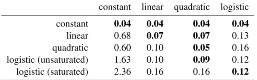
Table 3.1: Model selection experiment results. In each row, the data for the experiment was generated by the type of intensity model shown. Each column shows the registration error (in pixels) obtained when using that model in the column for the model-based similarity measure (best values are highlighted).
constant linear quadratic logistic
constant 0.04 0.04 0.04 0.04
linear 0.68 0.07 0.07 0.13
quadratic 0.60 0.10 0.05 0.16
logistic (unsaturated) 1.63 0.10 0.09 0.12 logistic (saturated) 2.36 0.16 0.16 0.12
Table3.1shows the registration errors for all 20 combinations between the five different intensity profiles used to generate the longitudinal images and four model types used for the intensity model estimation. Each row shows the registration error for one of the five generated datasets (lowest errors for each set are highlighted). The columns show the model used for estimating the intensity change over time forIˆ. The results show that the quadratic model is a good choice if the underlying true model is polynomial or the logistic model is not saturated; however, the logistic model is necessary when the true model is logistic and the time points are far enough to saturate the model.
3.3.3 Experiment 2: Synthetic Data
In this experiment, I created sets of 64×64 2D synthetic images (based on the Internet Brain Segmentation Repository (IBSR,2007) synthetic dataset). Each set consisted of 11 time points (Ii, i= 0, . . . ,10).I0was designated as the target image and all subsequent time points as the source images.
The gray matter intensities of all 11 images were fixed (Iigm= 80). For the source images,I1, . . . , I10, I introduced two types of white matter appearance change:
i) Spatially uniform white matter appearance change over time, starting as dark (unmyelinated) white matter (I1wm= 20) and gradually brightening (myelinated) white matter (I10wm= 180), resulting in linear contrast inversion between gray and white matter. The target white matter intensity was set to 100.
Iwm
1 ={50, . . . ,70}up toI10wm ={50, . . . ,200}). These gradients are of similar magnitude, as observed in the real monkey data (see Figure3.5).
I tested the similarity measures for two types of transformation models: affine and deformable with elastic regularization. Figure3.8shows the experimental setup with the deformable transformation model (for the affine registration experimentsΦiwas an affine transform; for the deformable registration experiment Φi was a longitudinal spline deformation with 20 control points). The aim of the experiment was to
recover the ground truth inverse deformation,Φ−i 1, by registering the 10 source images toI0(givingΦˆ−i 1) with each of the four similarity measures (SSD, NCC, MI, SSR). I repeated each experiment 100 times for each transformation model with different random deformations, giving a total of16 000registrations (2 white matter change×2 transformation model×10 source image×4 measure×100 experiment). Significance was calculated with Welch’st-test (assuming normal distributions, but unequal variances) at a significance level ofa= 0.01.
Next, I describe the results of the experiments for each transformation model.
target I0(1) I0(n)
I1 In error
Φi◦Φˆ−i 1
Φ1 Φn
ˆ Φ−i 1
1
2 3
4
1
0
Figure 3.8: Experimental setup: 1) Increasing white matter intensity gradient is added to the target,I0. 2) Adding known random longitudinal deformations yields the source images, 3) which are registered back to the target. 4) Registration error is calculated from the known (Φi) and recovered (Φˆ−1i ) transformations.
3.3.3.1 Affine transformation model
deformable solution. Therefore, I first investigate the sensitivity of affine registration to white matter appearance changes separately from deformable registration.
Figure3.9shows the results for registeringI1throughI10to the target imageI0 from multiple sets (n= 100, giving 1000 pair-wise registrations for each similarity measure) of longitudinal images with both uniform and gradient spatial white matter intensity profiles.
With uniform white matter, all four measures performed well when the contrast of the source image was close to the contrast of the target image (near 0 white matter intensity difference in the first plot of the median root means squared registration error). The results for the gradient white matter profiles show that the performance of both SSD and NCC declined as the gradient magnitude increased, while MI and SSR aligned the images well even with the strongest gradient. Overall, SSR significantly outperformed NCC and MI but not SSD; however, the differences between the overall registration errors are on the order of 0.001 voxels for SSD, MI, and SSR (see Table 1a. in Figure3.9).
The experiments suggest that affine registration can be reliably achieved by SSD, MI or SSR, but for simplicity MI should be used if affine alignment is the only objective.
3.3.3.2 Deformable registration
Similarly to the affine experiment, Figure3.10shows the error plots for deformable registrations in the presence of white matter intensity change. For uniform white matter, SSD again produced small registration errors when the contrast difference was small, but fared worse than MI and SSR in the presence of large intensity differences between the target and the source images. SSR performed slightly better than MI for all time points.
The setup with deformable registration and white matter gradient resembles the real problem closely and therefore is the most relevant. Here, SSD and NCC introduced considerable registration errors with increasing gradient magnitude. The registration error of MI remained under 2 voxels (mean = 1.62±0.45), while SSR led to significantly less error (mean =1.25±0.35) for all time points.
3.3.4 Experiment 3: Simulated Brain Data
−60 −30 0 30 60
0.01
0.03
0.05
WM intensity difference
median
rms
error
SSD NCC MI SSR
SSD NCC MI SSR
0.001
0.01
0.1
Mean Std 50th 90th
SSD 0.008 0.005 0.007 0.016 NCC 0.020 0.019 0.016 0.035 MI 0.012 0.005 0.011 0.018 SSR 0.010 0.009 0.007 0.020
Table 1a.
0.001 0.01 0.1
1 2 3 4 5 6 7 8 9 10
S N M m S N M m S N M m S N M m S N M m S N M m S N M m S N M m S N M m S N M m
target
Uniform
1 2 3 4 5 6 7
0.01
0.1
1
gradient magnitude
median
rms
error
SSD NCC MI SSR
0.01
0.1
1
Mean Std 50th 90th
SSD 0.205 0.277 0.015 0.670 NCC 0.092 0.090 0.041 0.244 MI 0.010 0.004 0.010 0.016 SSR 0.010 0.008 0.007 0.021
Table 1b.
0.01 0.1 1
1 2 3 4 5 6 7 8 9 10
S N M m S N M m S N M m S N M m S N M m S N M m S N M m S N M m S N M m S N M m
target
Gradien
t
−60 −30 0 30 60
0.5
1
1.5
WM intensity difference
median
rms
error
SSD NCC MI SSR
SSD NCC MI SSR
0
0.5
1
1.5
2
Mean Std 50th 90th
SSD 0.729 0.231 0.705 1.051 NCC 0.845 0.319 0.768 1.368 MI 0.767 0.222 0.754 1.059 SSR 0.637 0.176 0.623 0.886
Table 1c.
0 1 2
1 2 3 4 5 6 7 8 9 10
S N M m S N M m S N M m S N M m S N M m S N M m S N M m S N M m S N M m S N M m
target
Uniform
1 2 3 4 5 6 7
0 1 2 3 4 gradient magnitude median rms error
SSD NCC MI SSR
0 1 2 3
4 Mean Std 50th 90th
SSD 2.022 1.213 2.096 3.663 NCC 1.963 0.972 2.029 3.203 MI 1.306 0.521 1.329 1.949 SSR 0.609 0.187 0.588 0.859
Table 1d.
0 2 4
1 2 3 4 5 6 7 8 9 10
S N M m S N M m S N M m S N M m S N M m S N M m S N M m S N M m S N M m S N M m
target
Gradien
t
Figure 3.10: Experiment 1 results with deformable transformation. The graphs are set up similarly as in Figure3.9except all plots have linearyscales. The last setup with deformable transformation model and gradient white matter intensity is the most challenging and relevant to the real world problem.
3.3.4.1 Smoothing kernel size
In this experiment I investigated the effect of the smoothing kernel size on the registration accuracy of SSR. In addition to no smoothing, four isotropic median kernels with sizes 3, 5, 7, and 9 voxels were used to smooth the model parameters.
The size of the smoothing kernel had no significant influence on the global registration error (see Figure3.12), even though larger kernels tend to over smooth the salient features of the model, such as the boundary between the unmyelinated and myelinated white matter. No smoothing, on the other hand, allows areas of poor model estimation, due to misregistration between the time points, to remain in the intensity model. Most noticeably, initial misregistration near the gray matter white matter boundary can lead to a boundary shift.
Next, I illustrate this boundary shift with a 2D synthetic longitudinal dataset with a small misalign-ment between the time points shown in Figure 3.3. Assuming that this is the best initial alignment between the time points, the top row of Figure3.11shows the model images estimated from the dataset at timet2 with three different kernel sizes; the bottom row shows the registration results between the source (I2) and model images (Iˆ(t2)). As the kernel size increases, the model better approximates the true tissue intensities near the boundary and the registration error (boundary shift) decreases. While a large smoothing kernel is advantageous near the boundary, a smaller kernel is less likely to smooth out salient features within the white matter. Thus smoothing with an adaptive kernel size inversely proportional to the distance from the white matter boundary might be the most advantageous.
3.3.4.2 White matter segmentation
1
×
1
10
×
10
20
×
20
mo
del
ˆI(t
2
)
I2
registered
ground truth registered boundary
Figure 3.11: The effect of various median smoothing kernel sizes on the intensity model estimation and the subsequent registration (dataset is shown in Figure3.3).Top row:shows the estimated model from the misaligned synthetic longitudinal dataset with1×1,10×10, and20×20voxel kernels (the red outline is the correct tissue boundary). Bottom row:shows the results of elastically registering time point
I2to the modelsIˆ(t2)in the top row (the yellow outline is the boundary after the registration).
is lowest when the white matter mask is accurate or slightly underestimated, therefore accurate white matter segmentation is necessary.
3.3.5 Experiment 4: Monkey Data
I compared the model-based similarity measure to mutual information (MI) on sets of longitudinal magnetic resonance images of 9 monkeys, each with 4 time points (2 week, 3, 6, and 12 month). Each time point was affinely pre-registered to an atlas generated from images at the same time point (the atlas images for the four time points were affinely registered) and intensity normalized so that the gray matter intensity distributions matched after normalization (gray matter intensity generally stays constant over time). The tissue segmentation was obtained at the last time point with an atlas-based segmentation method (Styner et al.,2008).
1 3 5 7 9 0
1 2
smoothing filter size (voxels)
registration
error
(v
o
xel
s)
2wk 3mo 6mo
−3 −2 −1 0 +1 +2 +3
WM segmentation quality
Figure 3.12: Results for SSR registration with different median smoothing kernel sizes (left) and varying quality white matter segmentations (right; x-axis shows the amount of erosion (-) or dilation (+) applied to the accurate (0) white matter mask).
M−3 M−2 M−1 M0 M+1 M+2 M+3
none accurate brain
Figure 3.13: White matter segmentations used to investigate the influence of segmentation accuracy on SSR registration (erosion (M−·) and dilation (M+·) are applied to the accurate (M0) segmentation).
based on geometric considerations). The distance between transformed and target landmarks yielded registration accuracy. Figure3.15shows the experimental setup.
Note that for the model-based method the target image is notI12mo, but the modelIˆ12mo(t)estimated at timetof the source image. Here, the target image isI12moas white matter segmentation is easily obtained given the good gray matter white matter contrast, but other time points could be used.
2 wk
3 mo
6 mo
12 mo
Figure 3.14: Corresponding target (cyan) and source (red) landmarks for a single subject.
Table 3.2: Landmark registration error (in voxels) between target I12mo and source images
I2wk, I3mo, I6mo(significance level isα= 0.05; significant results are highlighted).
I2wk I3mo I6mo
mean std 50th 90th mean std 50th 90th mean std 50th 90th
MI 1.76 1.09 1.60 3.22 1.07 0.77 0.84 2.04 0.66 0.46 0.56 1.22 SSR 1.15 0.84 0.93 2.24 0.74 0.57 0.54 1.66 0.61 0.39 0.50 1.18
the model-based approach perform well in the absence of large intensity non-uniformity; however, SSR consistently introduces smaller erroneous deformations than MI.
Table3.2shows the aggregate results of the landmark mismatch calculations for both methods. The model-based approach can account for appearance change by adjusting the intensity of the model image (see the estimated model images in Figure3.15) and therefore is most beneficial when the change in appearance between the source and target image is large (I2wk,I3mo).
1 3 5 7
source model
original
SSR MI
Figure 3.15: Experimental setup for a single subject. To test MI, the source images (blue; from bottom:
I2wk,I3mo,I6mo) are registered to the latest time pointI12mo(green). The resulting deformation field and the magnitude of the deformations (in pixels) is shown in the right panel. For SSR, the source images are registered to the model (red) that estimates the appearance ofI12moat the corresponding time of each source image (results in middle panel). The results are evaluated using manually chosen landmarks in the target and source images (not shown here).
3.4 Conclusions
2 wk 3 mo 6 mo 12 mo
source target
SSRerror <MIerror
SSRerror >MIerror
SSRerror = MIerror
CHAPTER 4
Quantitative MRI Atlas of Postnatal Rhesus Macaque Brain Maturation
4.1 Introduction
The maturation of the mammalian brain relies on a tightly coordinated sequence of cell proliferation, cell positioning, axonal growth and pruning, and the elaboration of the myelin sheath of the axons (myeli-nation). The spatial and temporal trajectories of brain maturation and cognitive development are driven by genetics, environmental factors, and learning, and vary considerably between individuals (Knickmeyer et al.,2008). While most mammalian organ systems fully develop in utero, the brain continues to develop and acquire new functionality well after birth. The resulting plasticity of the immature brain enables organisms to rapidly adapt to their environment (Zilles,1992), but it also leaves the brain vulnerable to developmental insults (McEwen,1994). A variety of toxic, infectious, vascular, traumatic, and psy-chological insults have been shown to alter the normal trajectory of brain development (Riley et al., 2011;Rees and Inder,2005;Morton et al.,2017;Friess et al.,2007;Lupien et al.,2009). In addition to these early postnatal insults, there has been a growing interest in studying normal brain maturation and neurodevelopmental disorders, such as autism spectrum disorders and schizophrenia, with the aid of non-invasive medical imaging technologies (Toga et al.,2006).
0.5 3 6 12 18
0.5
3
6
12
18
0.5
3
6
12
18
0.5
3
6
12
18
0.5
3
6
12
18
0.5
3
6
12
18
Figure 4.1: Axial slices of MR brain images of monkey at ages 2 weeks, 3, 6, 12, and 18 months. White matter appearance changes non-uniformly as axons are myelinated during brain development.
changes (Barkovich et al.,1988). The combined morphological and appearance changes (see Figure4.1) make longitudinal analysis of brain development a challenging problem. Longitudinal analysis has to be flexible enough to allow for the large non-uniform morphological and appearance changes, while at the same time provide temporally smooth solutions.
Animal models, ranging from rodent to non-human primate, have been widely used in comparative human brain development studies. Non-human primate models have been especially important, due to their phylogenetic proximity to humans and their similar brain architecture, prolonged gestational period, developmental trajectories, complex cognitive function, and social behavior (Capitanio and Emborg, 2008). While chimpanzees are our closest non-human relatives, practical considerations have led to the use of more distantly related primate species as the predominant research subjects (Lacreuse and Herndon,2008). In fact, an old world monkey species, the rhesus macaque, is the most widely used non-human primate model (Carlsson et al.,2004) and it has even been the subject of a series of infamous landmark studies that have changed how we approach child-rearing to this day (Harlow et al.,1971).
finding the developmental age of brain regions (Dean et al.,2015), describing atypical development (Just et al.,2012), or aiding registration (the topic of Chapter5). While longitudinal atlases for morphological changes have been developed, there are few atlases that capture the longitudinal appearance change of the developing brain, especially atlases that target prenatal and early postnatal brain development – periods when image registration and segmentation are especially difficult. This is not surprising, given the challenging nature of longitudinal imaging in utero and during early postnatal development. Existing brain atlases targeting this period have focused on bulk measures, such as volumetric changes of seg-mented regions (Gilmore et al.,2011), or on morphological changes only. However, a number of atlases summarize other quantitative measures of brain maturation (most often diffusion characteristics hinting at the underlying structural organization) for small mammals (Zhang et al.,2005;Huang et al.,2008; Chuang et al.,2011) and primates (Hikishima et al.,2013), including humans (Sadeghi et al.,2013;Dean et al.,2014,2015;Makropoulos et al.,2016). Of these atlases, most are using built cross-sectional images and only Dean et al. provides a voxel-wise longitudinal estimation of diffusion characteristics (Dean et al.,2015). Even so, out of the 209 human subjects used by Dean et al., more than half have a single time point and only five have four time points (compared to our study with five time points for each subject).
4.2 Estimating the Atlas from a Population
To build the atlas, I made the following choices and assumptions:
1. Locality of the model.The model is defined over a white matter mask only as the expected change
in gray matter intensity throughout neurodevelopment is negligible compared to the white matter.
2. Atlas space.As white/gray-matter contrast is best for a fully matured brain, the atlas is defined on
an average atlas image for the latest time point in our dataset – where an automatic white matter segmentation can be reliably obtained. The atlas model parameters are resampled in the anatomical space of each subject through registering the atlas to the latest time point.
3. Temporal model type.Ideally, the model should be learned fully from the data. However, given
2 weeks 6 months 18 months
Figure 4.2: Example of an expert-defined anatomical landmark within the same subject (top:axial slices;
bottom:sagittal slices).
intensity). This way the temporal model is parameterized by only two parameters capturing onset and rate of maturation.
4. Spatial regularization.In order to provide robust estimates of the model parameters with respect
to image noise and small registration errors, spatial regularity is enforced on the estimated group-wise model parameters via a3×3×3median filter.
4.2.1 Monkey Dataset
The images were inhomogeneity corrected (Tustison et al.,2010) and registered into a standard-ized atlas space using an affine transformation with a local cross correlation metric (ANTS (Avants et al.,2009)). Skull stripping and tissue segmentation were obtained with an atlas-based segmentation method (Styner et al.,2008). Furthermore, 35 anatomical landmarks were defined by an expert for all 5 time points (see Figure4.2).
To build the maturation atlas intra-subject elastic deformable registration to the latest time point is performed first using the previously developed longitudinal SSR registration in Chapter3. Inter-subject registration is then established by registering the oldest time point of each subject to a common atlas space. This establishes correspondences between all subjects for all time points. I thin the white matter mask to avoid model estimation errors for the logistic intensity model near tissue boundaries, due to partial voluming, segmentation errors, or registration errors. For each point in the thinned white matter mask the logistic models are then estimated as follows.
4.2.2 Model Estimation
For the point-wise estimation of logistic curves, I considered (i) a direct fit of a single logistic model to all data points (disregarding their longitudinal nature), (ii) a full longitudinal estimation procedure, and (iii) fitting individual logistic curves for each subject followed by the computation of the median of these logistic curves. Since different subjects of the same age may be at slightly different stages of neurodevelopment, the first two approaches would require a simultaneous estimation of this time-shift to avoid underestimating the maturation rate. I, therefore, chose the latter approach as it is robust to such time-shifts, is simple, and provides a parametric model. I locally compute the median curve over the population, using the approach proposed for calculating the functional boxplot (Sun and Genton,2011), where I replace all the measured values by the values of their individual logistic model fits. As the median curve will be a curve from the dataset, I thus obtain a median logistic curve. (This is fundamentally different from computing a point-wise median.) The individual logistic models are fit using ordinary least squares1[θˆ
j =argmin θ
P
i(Ij(ti)−logistic(ti, θ))2], whereIj(ti)is the intensity at time pointti
1
for subjectjandθdenotes the coefficients for the logistic model. The logistic model is defined as
logistic(x, t;α, β(x), k(x)) = α
1 +e−k(x)(t−β(x)) , (4.1)
whereαis a global parameter (intensity change between unmyelinated and myelinated white matter),
β (onset: time of maximum rate of intensity change) and k(maximum rate of intensity change) are
spatially varying model parameters (see Figure4.3). I further compute the variance of the actual measured values with respect to the median logistic model (θ) at the ages of interest [ˆσ2(ti) = N(1ti)Pj(Ij(ti)− logistic(ti, θ)))2], whereN(ti)denotes the number of measurements at time pointti. This allows us to
introduce local weights into the registration method described in Chapter5.
t i
2w 3m 6m 12m 18m
α
Figure 4.3: Logistic intensity model.
As maturation is expected to be locally smooth, I smoothly extend the estimated parameters of the logistic model to the full white matter mask. Figure4.4shows sample slices with the color-coded coefficients for onset and maturation rate.
Shortcomings of the model estimation. Time-shift uncertainties are only implicitly accounted for in
the model, as the computed variances will be a combination between image noise, registration errors, and time-shifts of the maturation trajectories. An improved estimation procedure could also estimate the time-shifts, however at the cost of greater model complexity. The observations indicate that these shifts (if present) are relatively minor and therefore I chose not to explicitly model them.
4.2.3 Comparison to Expected Myelination Pattern
100 200 300 in tensit y 2w 18m 100 200 300 age in tensit y β (onset) k (rate) 4 0 -4 4 2 0
Figure 4.4: Estimated onset (in months) and rate of maturation overlaid on three axial slices of the structural atlas (columns 1-3: inferior to superior). Note that this is the initial estimate in the thinned white matter mask. The parameters follow an expected pattern of maturation. The plots show the individual (red) and median (blue) logistic curves and the intensity values (black dots) for the ten subjects for two different voxels.
chronological pattern of the maturation atlas of the macaque model to the patterns defined in previous histochemical and MR studies of myelination in humans.
Overall, the maturation atlas captures the expected maturation patterns, with areas deeper in the brain either reaching their matured intensity early or already being fully matured at two weeks of age (first time point). On a finer scale, several complex rules govern the spatial and temporal sequences of myelination as described in (Kinney et al.,1994):
1. Myelination proceeds from the center to the periphery:proximal pathways myelinate earlier
and faster than distal ones.
2. Myelination proceeds from back to front:occipital poles myelinate before frontotemporal poles.
3. Some structures myelinate early on: at birth, the following cerebral structures are partially
myelinated: cerebral peduncle, internal capsule, central corona radiata.
4.3 Conclusions