Do active communities support activity, or support active people? : residential self-selection in the estimation of built environment influences on physical activity

(1)

Janne Boone-Heinonen

A dissertation submitted to the faculty of the University of North Carolina at Chapel Hill in partial fulfillment of the requirements for the degree of Doctor of Philosophy in the Department of Nutrition

(Nutrition Epidemiology), Gillings School of Global Public Health

Chapel Hill 2009

(2)

ii

(3)

Janne E. Boone: Do active communities support activity, or support active people? Residential self-selection in the estimation of built environment influences on physical activity

(Under the direction of Penny Gordon-Larsen, PhD)

In a growing body of research, the built environment, composed of “neighborhoods, roads, and buildings in which people live, work, and play,” has been shown to be related to physical activity. While promising for physical activity promotion, substantial limitations must be addressed before built environment research can adequately inform policy recommendations. To this end, we focused

on three methodological challenges of particular concern for built environment research: (1)

quantitative characterization of a complex environment, (2) confounding by other inter-related

environment characteristics, and (3) residential self-selection bias resulting from systematic

sociodemographic and behavioral differences among individuals selecting different types of

neighborhoods. We used data from the National Longitudinal Study of Adolescent Health, a

nationally representative cohort of over 20,000 adolescents followed over seven years into young adulthood. A large scale geographic information system (GIS) linked community-level built (e.g., recreation facilities, land cover, street connectivity) and socioeconomic (e.g., median household income, crime rate) environment characteristics to individual-level sociodemographic and behavioral data in space and time.

Using factor analysis, we identified several built and socioeconomic environment constructs. We found that the socioeconomic environment is a potentially important confounder of built

(4)

iv

represent general density of development. Lastly, in longitudinal analysis, we observed an increase in physical activity among males with a greater number of physical activity-related pay facilities and a decrease in physical activity among males and females with higher neighborhood crime rate. Other built environment characteristics were unrelated to physical activity. Additional analysis suggests that residential self-selection can attenuate, as opposed to magnify, environment-physical activity associations.

(5)

(6)

vi

Acknowledgements

There are many people whose advice, guidance, encouragement, support, and honest criticism have made this dissertation possible. Dr. Penny Gordon-Larsen has provided each of these things when I needed them most. She encouraged me to follow my research interests, introduced new topics and methods when my interests waned, and gently yet unmistakably pushed me to complete projects when my interests waned too much. She was always available to talk through ideas whether good or bad, work through painfully detailed analytical decisions, and review my chronically too-long manuscripts. She is a gifted mentor and a wonderful friend, and has taught me so much about research, life, and how to balance the two.

I am also grateful for my other committee members: Dr. Barry Popkin for his forthright criticism and endless enthusiasm, Dr. Kelly Evenson for providing rigorous feedback and for keeping me excited about the field, Dr. David Guilkey for his patient guidance with even the most basic econometric methods, Dr. Yan Song for providing conceptual and methodological perspectives from urban planning, and Dr. Linda Adair for asking challenging questions and always keeping her door open.

(7)

EH00380), Robert Wood Johnson Foundation Active Living Research program, and Henry Dearman and Martha Stucker and the Royster Society of Fellows at the University of North Carolina at Chapel Hill. Their support of young investigators opens opportunities for not only their grant recipients but also the advancement and evolution of health research.

I thank my family and friends for their virtually unconditional support over so many years. My parents have supported and encouraged me, listened to my generally self-inflicted problems, instilled an appreciation for hard work and contributing to the world around me. Friends at UNC and around the country helped me to, sometimes by force, laugh, relax, and remember that there is more to life than regression modeling. Finally, thank you to Chris, my husband who loves and supports me every minute of every day.

(8)

viii

Table

of

List

of

Tables

Table 1. Built and socioeconomic environment measures:1_{data sources and variable descriptions ... 47} Table 2. Individual-level characteristics by sex [mean/% (SE)]1 ... 49 Table 3. Built and socioeconomic environment characteristics: descriptive statistics1_{... 50}

Table 4. Built environment factor loadings resulting from exploratory factor analysis1_{... 51}

Table 5. Socioeconomic environment factor loadings resulting from exploratory factor analysis1_{.... 52} Table 6. Crude associations between built environment factor scores and socioeconomic environment factor quartiles [coeff (95% CI)]1_{... 53} Table 7. Assessment of confounding to associations between built and socioeconomic environment factor score quartiles and weekly bouts of MVPA, males (n=8,747) [exp(coeff) (95% CI) [change in coefficient2_]1_{... 54} Table 8. Assessment of confounding to associations between built and socioeconomic environment factor score quartiles and weekly bouts of MVPA, females (n=8,694) [exp(coeff) (95% CI) [change in coefficient2]1 ... 56 Table 9 Association between representative built, social, and economic environment measure

quartiles and weekly bouts of MVPA [exp(coeff)]1_{... 58} Table 10. Sociodemographic characteristics in adolescence and young adulthood: descriptive

statistics, by residential relocation status [mean/% (SE)]1_{... 73} Table 11. Baseline and changes in built and socioeconomic environment characteristics between adolescence and young adulthood: descriptive statistics, by residential relocation status1 ... 74 Table 12. Random and within-person effect estimates1_{of built and socioeconomic environment} characteristics on MVPA between adolescence and young adulthood [elasticity (95% CI)] ... 75 Table 13. Variation in within-person effect estimates1_{of built and socioeconomic environment} characteristics on MVPA between adolescence and young adulthood by residential relocation status,2 [elasticity (95% CI)] ... 76 Table 14. Model coefficients and significance for random and within-person effect estimates1_of built and socioeconomic environment characteristics on MVPA between adolescence and young adulthood ... 77 Table 15. Model coefficients and significance for within-person effect estimates1_{of built and}

(13)

List

of

Figures

Figure 1 Relationships among diet, physical activity, and obesity within the socio-ecologic

(14)

xiv

List

of

Abbreviations

Add Health National Longitudinal Study of Adolescent Health CFA Confirmatory Factor Analysis

CI Confidence Interval

EFA Exploratory Factor Analysis

ESRI Environmental Systems Research Institute FIML Full Information Maximum Likelihood GIS Geographic Information Systems GPS Global Positioning System ICC Intraclass Correlation

MVPA Moderate to Vigorous intensity Physical Activity

PA Physical Activity

PCA Principle Components Analysis RMSE Root Mean Square Error SES Socioeconomic Status U.S. United States

(15)

A. Background

Evidence that built environment features such as parks and connected street networks can support active lifestyles holds tremendous promise for increasing physical activity levels and

preventing obesity. Ultimately, built environment characteristics shown to influence physical activity can be used promote active lifestyles. However, substantial methodological limitations in existing research need to be addressed before this literature can adequately inform policy recommendations.

Potential residential self-selection bias, or bias resulting from already active individuals selecting activity-supporting neighborhoods, is considered a primary threat to causal inferences regarding the influence of the built environment on physical activity. Existing research is dominated by cross-sectional designs and little is known about the magnitude or direction of residential self-selection bias. Longitudinal designs can control for residential self-self-selection due to observed characteristics and unobserved characteristics that remain constant over time (e.g., inherent

motivation to exercise) using fixed effects models or similar methods. The few existing longitudinal studies focus on changes in health and behavior following residential relocation, yet the environment can change around stationary individuals and exclusion of residentially stable households could lead to selectivity bias. However, cohorts with time-varying environment and individual behaviors have not previously been available.

(16)

2

effects, but understanding of these complexities is limited due to the small range of built environment characteristics included in most studies. Furthermore, built environment patterning may shift across life stages but has not been studied in adolescents.

For the proposed research, we addressed these limitations by leveraging a unique Obesity and Environment database that comprises the first large scale geographic information system (GIS) to link community- and individual-level data in both space and time in a large ethnically diverse sample. The National Longitudinal Study of Adolescent Health (Add Health), a prospective cohort followed from adolescence to young adulthood, provides extensive individual-level health behavior and outcome data, as well as detailed time varying data on a wide range of community-level factors such as land use, recreation facilities, economic, climate, and crime data.

B. Research

Aims

The overarching goal of this research was to estimate the influence of diverse built

environment characteristics on physical activity during adolescence and young adulthood in a racially and ethnically diverse sample. We achieved this goal through the following aims:

1) Describe the inter-relationships between built and socioeconomic environment

characteristics in a nationally representative sample of adolescents.

a. Using exploratory factor analysis, identify multidimensional built and socioeconomic environment constructs from a large set of objective environment measures.

b. Quantify the extent to which inter-related environment constructs confound cross-sectional, multivariate associations with physical activity.

c. Create replicable measures for use in longitudinal analysis that account for inter-relationships and avoid collinearity.

2) Estimate longitudinal effects of the built environment on physical activity and explore the

(17)

a. Use fixed effects models to estimate effects of several built and socioeconomic environment characteristics on physical activity while controlling for time invariant, unmeasured

characteristics.

b. Assess the influence of residential self-selection bias due to time invariant, unmeasured characteristics on estimated environment-physical activity associations by comparing fixed effects and naïve estimates.

(18)

II. Literature Review

The domestic (1-3) and global (4) increase in obesity prevalence and its associated

morbidities and mortality (5-7) are well known. Individual-level obesity prevention strategies have achieved limited success (8), and recent attention has turned to broad environmental factors as targets for obesity prevention. In particular, associations between physical activity and community design characteristics have generated not only rapid growth in public health and transportation research (9-13), but also shifts in practice such as the creation of “new urbanist” neighborhoods and application of smart growth principles to community planning (14, 15).

However, research on environmental determinants of obesity and associated behaviors is in its infancy, warranting more detailed examination of these relationships in population subgroups and elucidation of methodological shortcomings in existing research. Without additional research that fill these methodological and conceptual gaps, policies and existing practices designed to encourage physical activity through changes to the built environment will remain without a solid scientific evidence base.

A. Determinants of Physical Activity

A rapidly growing body of research examines the role of a vast range of contextual factors in influencing how individuals move throughout the day (16, 17). The socio-ecologic framework in Figure 1 depicts one major pathway linking behaviors to obesity, chronic disease, and related risk

factors. While this example simplifies complex obesity and chronic disease etiologies, it is useful for theorizing and testing behavior determinants across levels of influence.

The socioecologic framework

(19)

behav (18). know (21), o

the m 24). T past d with l While levels Figur frame Adapt Obesit viors: intraper Historically, wledge (19) an or organizatio

While neig majority of nei

The importan decade, startin living in a dis e each level c s and is argua

re 1 Relation ework

ted from model ty, Weight Gai

rsonal, interpe health behav nd motivation onal factors, s ghborhoods c

ghborhood he nce of multipl

ng with resear sadvantaged n an be influen bly the ultima

nships among

l developed at in, Diet, and Ph

ersonal, instit vior interventi (20), or inter such as workp

an capture int ealth research e levels of inf rch showing i neighborhood nced by any ot ate goal of mo

diet, physica

the National H hysical Activity

tutional/organ ions have focu rpersonal fact place support ter-personal i h focuses on b

fluence in pub increased coro d, independent

ther level, pub ost neighborh

l activity, and

Heart, Lung, an y; August 2004

nizational, com used on intrap tors such as in ts like onsite f influences (e. built and socio

blic health (2 onary heart d t of individua blic policy ca hood health re

d obesity with

nd Blood Institu 4, Bethesda M

mmunity, and personal facto nfluence of a

fitness equipm g., social supp oeconomic en 5) has been r disease inciden

al socioeconom an potentially

esearch (27, 2

hin the

socio-ute Workshop: MD

d public polic ors such as

spouse’s beh ment (22).

(20)

6

The built and socioeconomic environments

The built environment is a major component of community design comprised of aspects such as buildings, transportation systems, parks, and greenways. It is a particularly promising target for improving population health due to its apparent influence on physical activity and hence chronic disease prevention, as well as its existing linkages with local policies.

Researchers have found relatively consistent relationships between physical activity and urban sprawl (29), alternatively referred to as “walkability” (30), incorporating street connectivity measures, land use mix, housing density, and block lengths or retail floor area. Associations between physical activity and pedestrian and biking infrastructure such as sidewalks and bike lanes have been mixed (31, 32). Physical activity is related to access to recreational resources such as parks or physical activity facilities in youth (33) and adults (34, 35). Retail destinations such as shops and restaurants within walking distance are also correlated with walking behaviors (31, 36).

The socioeconomic environment, comprised of economic factors (e.g., poverty rate) and social factors (e.g., racial composition or crime and safety), are related to physical activity, obesity, and disease in existing research (37, 38).

Dynamic interactions within and between levels of influence

The socio-ecologic framework accommodates dynamic relationships among factors within and between levels of influence. Aspects of the built and socioeconomic environments are correlated (33) and appear to have independent relationships with physical activity (37). Built and

socioeconomic environments may also interact: for example, high income neighborhoods may have greater local political influence to lobby for a community center or traffic calming measures, which could theoretically maintain or build social capital and improve socioeconomic indicators in the long run.

(21)

engaging in physical activity (intrapersonal factor), act as a visual reminder to be active, or enforce activity as a cultural norm (interpersonal factors) (39). While we do not address perceived measures of the environment in our research, we assume any causal influence of the objective environment on physical activity occurs at least in part through perceptions of the environment (18), thus involving both intra- and interpersonal level factors. While agreement between perceived and objective measures of the environment is low (40, 41), the socio-ecologic framework remains useful as agreement may improve with better characterization of neighborhood boundaries and amenities.

Further, the dynamic relationships among socio-ecologic framework levels imply that intra- and interpersonal factors influence community-level exposures, either through changes in the environment around stationary residents, residential relocation, or some combination of the two. By way of simple example, the first mechanism (changes in the environment) would occur if the city opened a new basketball court in response to demand by community members. The second mechanism (residential relocation) would occur if those motivated to exercise choose to move into neighborhoods with parks or close access to fitness facilities. The latter example describes a major criticism of neighborhood health research and one focus of our study: residential self-selection (42). In other words, our concern about self-selectivity raises the question of whether addition of recreation options will enhance activity patterns in any selected neighborhood.

B. Research Gaps

Discussions of challenges and limitations to neighborhood health research have been previously published (42, 43). Of particular relevance to this project, heterogeneity of relationships by life stage and gender has been largely ignored, and many studies are conducted in small

geographic areas with limited geographic variability and environment measures. Further, the literature is largely cross-sectional, which is particularly vulnerable to bias due to residential self-selection. We discuss each of these issues in the following sections.

(22)

8 Study populations used in existing research

Adolescence and young adulthood

Physical inactivity is an exceptionally consistent risk factor for obesity in both children (44, 45) and adults (46, 47). Additionally, as physical activity declines dramatically throughout

adolescence (48-51) and young adulthood (52), obesity prevalence rises in parallel (53-56). The transition from adolescence to young adulthood is thus a critical period for weight gain as well as behavior change (53, 57-59), making this life stage a promising target for obesity prevention.

The majority of research on built environment effects on physical activity has focused on adults, and findings in child, adolescent (10, 33, 60), and elderly (61, 62) populations are largely similar with some key exceptions. Contrary to findings showing “sprawl” as a barrier to physical activity (63, 64), Nelson and colleagues reported higher physical activity in adolescents living in suburban neighborhoods (65). Likewise, de Vries and colleagues identified the number of parallel parking spaces as a positive correlate of physical activity in grade school children, theorizing that they may create an additional buffer between the sidewalk and street or reduce vehicle speed (66). Additionally, traffic safety appears to be a stronger predictor of active commuting (67, 68) and physical activity (69) in children than adults. These studies suggest that built environment characteristics supporting physical activity may be sensitive to the age of the target population. However, built environment research in children and adolescents is growing but still limited.

Sex differences

Differences in determinants of physical activity between males and females (70) may be even more pronounced in adolescence, when participation in organized physical activity is higher in males (71). Females may also be more influenced by safety concerns (72) and sociodemographic

(23)

Health population in previous studies (74). However, few studies have examined sex-specific associations or sex interactions between the built environment and physical activity.

Geographic scope

Further, most existing research has been conducted in samples derived from confined

geographic areas with limited racial and ethnic diversity (e.g., (14, 31, 61, 75)), making generalization of findings difficult. Study of built environment-health relationships in large, sociodemographically diverse samples residing in diverse environmental contexts, particularly in critical age groups, is an essential prerequisite to creating policies and environments that support physical activity.

Interrelationships between built environment characteristics

Neighborhood environments are extremely complex, composed of a multitude of inter-related characteristics. Correlations between environmental characteristics pose two problems for assessing relationships with behavior. From a statistical perspective, traditional multivariate methods

incorporating inter-related independent variables are susceptible to multicollinearity and violation of model assumptions. From a conceptual perspective, single characteristics likely operate not in isolation but as combinations of design features. Examination of patterning among environment variables is valuable not only for understanding how, and to what extent, environment characteristics are inter-related, but also for developing environment measures which account for inter-relationships and avoid multicollinearity.

Several methods can be used to examine inter-relationships among variables, including descriptive approaches, cluster analysis (or its maximum likelihood counterpart, latent class analysis), creation of summary variables that optimize relationships with an outcome of interest, and

(24)

10

mutually exclusive groups with similar patterning among numerous variables. For example, Nelson et al identified several clusters of adolescents characterized by various patterns of built and

socioeconomic environment measures such as newer suburban and low socioeconomic status inner-city areas (65). However, the resulting patterns are categorical and data-driven, and thus not easily applied to longitudinal analysis or replication in external populations.

Additional approaches include index measures and reduced rank regression, which create summary variable(s) that explain the maximum amount of variance in the outcome variable(s). Indeed, to account for correlations between measures of urban form, Frank et al (30) developed a walkability index incorporating net residential density, street connectivity, and land-use mix; these components were weighted in a manner that maximized the explained variance in accelerometer-measured moderate physical activity duration per day. This walkability index has been examined in other samples (76), a necessary step because they were created by optimizing relationships with the outcome of interest. However, this walkability index does not incorporate recreational resources such as parks or fitness centers, which are also important elements of the built environment.

(25)

More generally, with these and few other exceptions (32, 61, 65), existing studies consider a single dimension of the built environment in relation to physical activity rather than the combined effect of multiple dimensions. Given the wide range of built and socioeconomic characteristics that are associated with physical activity, even characteristics weakly correlated enough to avoid multicollinearity may confound associations with physical activity. Therefore, concerns about multicollinearity and confounding must be balanced when estimating independent (or joint) effects of environment characteristics on physical activity.

In sum, greater understanding of how a broad range of built and socioeconomic environment characteristics are inter-related in demographically and geographically diverse adolescent populations is needed. Such knowledge will inform strategies to better account for correlations and potential confounding among environmental variables when estimating their independent associations with physical activity.

Residential selfselection: a major research gap

Potential bias due to residential self-selection has been identified as the primary limitation in built environment research (77) and is of particular concern in cross-sectional studies which

predominate the existing literature. We refer readers to two excellent reviews on residential self-selection in the context of travel behavior: Bhat and Guo discuss several adjustment methods of control for residential self-selection and present their own simultaneous modeling strategy (78), and Mokhtarian and Cao review methodologies used to address “attitude-induced” residential self-selection, which is driven by travel or residential preferences (79). The following discussion builds on these reviews by incorporating perspectives from health research using epidemiologic and econometric methods.

(26)

12

indirectly related to the exposure and outcome. In the context of built environment effects on physical activity, bias resulting from a direct relationship will result if already physically active individuals select neighborhoods based on their activity-supporting amenities. As an example of indirect relationships which may lead to bias, low income families may choose a neighborhood based solely on the affordability of housing; if these neighborhoods also contain inadequate physical activity resources and the families are less physically active (33), the built environment–physical activity relationship can be overestimated. Put simply, positive relationships between the built environment and physical activity can be attributed to (1) the effect of the environment on physical activity, (2) the effect of predisposition for physical activity, or characteristics related to physical activity, on residential choice, or (3) both.

Formally, consider the following model of physical activity (PA) as a function of vectors of environmental exposures of interest (E), sociodemographic characteristics (S), measured residential preferences (P), and unmeasured or unmeasureable characteristics that are related to PA (U). ε is an error term assumed to be random.

(1) PA = β0 + β1E + β2S + β3P + β4U + ε

Typical analysis of associations between the built environment and physical activity include PA, E, and S using traditional multivariate adjustment of common sociodemographic measures. Some studies include P, which capture measured residential preferences that may influence residential choice. However, U is unmeasured and is thus omitted from the model, and variability in PA

explained by U must be relegated to the error term in the model to form a composite error ε*=β4U+ ε. This is permissible if U is unrelated to E, S, and P. However, if ε* is correlated with the independent variables, standard estimation methods will lead to biased estimates of the built environment variable coefficients (β1) while also potentially distorting the estimates of the remaining coefficients in the equation (β2, andβ3). Understanding these complex inter-relationships is essential for obtaining precise, robust, and unbiased estimates of neighborhood effects (80).

(27)

for neighborhood characteristics related to physical activity amenities or other features such as schools, proximity to work or family, or other factors. These components may lead to residential self-selection bias, described as unmeasured confounders by epidemiologists and unobserved

heterogeneity by economists (81).

Direct evidence of residential selfselection

Largely, the literature on environmental determinants of physical activity and obesity treats residential decisions as exogenous factors. However, the strong roles of race and income in

residential selection are well documented in migration and residential mobility research (82, 83) as well as housing selection studies (84, 85). Coupled with the vast literature demonstrating

socioeconomic and racial disparities in physical activity (86), existing knowledge supports the indirect residential self-selection bias mechanism. Further, recreation and other physical activity-related facilities are inequitably distributed across neighborhoods by race-ethnic and SES composition (33).

There is also evidence for the direct residential self-selection bias mechanism. For example, a recent market survey supports increasing yet varied preferences for denser, more centrally located neighborhoods (87). Consumers who prefer such neighborhoods might tend to have higher physical activity levels. Indeed, participants citing access to transit as an important reason for living in a “transit-oriented development” were almost 20 times more likely to use rail transit than those who did not cite this reason (88). Likewise, physical activity and belief that an activity-friendly community will support active transit have been shown to be significant predictors of desiring to live in an activity-friendly community (89). The microeconomic behavioral literature suggests that there may be peer neighborhood effects leading to self-selection or preference for neighborhoods resulting in race/ethnic stratification across neighborhoods, even in the situation of equivalent expenditures (and potentially amenities) across these neighborhoods (90).

(28)

14

preference, belief, and behavior data which have important limitations. First, residential choices are determined by a virtually infinite set of variables such as affordability, convenience, and proximity to social support networks that may not be articulated by respondents, so reporting preference for activity-supportive communities has limited meaning (85, 91). Second, preferences are endogenous; unobserved factors such as financial constraints (i.e. affordability) may influence both self-reported preferences and selection of neighborhoods with amenities of interest. Failure to control for the endogeneity of preferences can result in biased estimates for the preference variables.

Strategies to control for residential selfselection bias

Associations between built environment factors and behavioral outcomes have been the topic of investigations across several fields including urban planning, transportation, economics, and epidemiology, each with their own methodological norms, culminating in recent and increased interdisciplinary research (9, 11, 92). To adjust for residential self-selection bias, these researchers have taken various approaches, including adjustment for self-reported residential preferences, adjustment for observed predictors of residential selection, longitudinal designs, and structural equations modeling.

While randomized controlled trials that experimentally assign families or amenities to neighborhoods (93) may help to address residential self-selection bias, experimental assignment of neighborhoods (or neighborhood characteristics) is not often financially or politically feasible. Therefore, we focus on advancements in statistical adjustment methods, availability of richer, longitudinal environmental datasets, and innovative study designs that have, and can continue to, vastly improve the validity of observational studies.

(29)

variables in multivariate models(94, 95)or to create variables reflecting the dissonance between residential preferences and objective neighborhood characteristics (96-98).

While these methods are innovative, they require the assumption that preference measures capture true preferences and are not influenced by current environment or transportation behaviors. As we have described, such assumptions may not hold. In studies of built environment determinants of physical activity, preferences and attitudes pose problems beyond those described for studying residential choice. Many economists view an individual’s attitudes and preferences as being determined by many of the same factors that determine physical activity and residential selection. Additionally, reporting errors associated with self-reported preferences and behaviors are probably strongly correlated: those who value public transit might be more likely to over-state both their preference for and use of public transit. That is, unobserved factors (U and V) affect both preferences and self-reported physical activity-related behaviors.

For these reasons, self-reported residential preferences are likely endogenous and thus inadequate as control variables in the prediction of self-reported physical activity. There is a large literature on the topic of determinants of preference structure which is outside the purview of this discussion. Ultimately, it is possible that controlling for residential preferences may not only fail to correct for residential self-selection bias but may introduce additional bias due to correlation of errors in reported preferences and behaviors. While self-reported preferences may provide insights about the potential role of preferences in residential choice, this approach is not a substitute for other methods which are less vulnerable to endogeneity and correlated measurement errors.

Control for observed predictors of residential selection. An alternative approach is to control for

(30)

16

walkability measures and walking were attenuated after propensity score adjustment, in some cases near or past the null (15).

Propensity score methods model “treatment,” defined in this context as living in a

neighborhood with activity-supportive characteristics, as a function of measured covariates. These strategies model the probability of living in a particular environment, given individual characteristics. Resulting probabilities (propensity scores) are subsequently used as adjustment or matching variables in models predicting physical activity from environment characteristics. Propensity score methods were developed for binary treatments but can be expanded to multiple-level treatments. However, these methods are not always easily implemented. Indeed, Boer et al were forced to conduct a series of analyses comparing adjacent levels of built environment measures, adjusting for propensity scores reflecting the probability of living in areas with higher versus lower measures within each pair of levels (15). Alternatively, predicted probabilities can be incorporated into weighting variables (inverse-to-probability-of-treatment weighting), which offer the advantage of accommodating multi-level or continuously scaled “treatments” (101).

There are several advantages of propensity score methods over traditional covariate

adjustment. The balance of covariates can be explicitly verified, and larger sets of covariates can be included in analysis. In the case of matching and weighting methods, selection bias induced by conditioning on common effects of the outcome and exposure (e.g. residential movement) can be avoided (102). However, propensity score methods only control for observed characteristics and assume adequate measurement of included variables. Therefore, they can control for residential selection bias only to the extent that covariates included in the treatment models capture determinants of selection into activity-supportive neighborhoods (103, 104). Unobserved characteristics correlated with the environment and physical activity will bias the obtained estimates. Thus, propensity score methods may not fully address residential self-selection.

(31)

physical activity in relation to changes in the built environment. For example, Krizek took advantage of an annual panel survey that followed households who moved within a metropolitan area (105). Krizek used first difference models to estimate change in travel behavior as a function of change in the built environment resulting from residential relocation, finding that an increase in neighborhood accessibility was associated with a decrease in vehicle miles traveled. This study design controls for endogenous characteristics such as motivation for physical activity that remain constant over time by subtracting out time invariant components of U in the model above. To illustrate, consider an expansion of Model 1, which distinguishes variables that change (time variant) versus remain constant (time invariant) for individual i over time t:

(2) PAit = β0 + β1Eit + β2Si + β3Tit +β4Pi + β5Ui + β6Vit + εi + νit

S and T are vectors of observed time invariant and variant sociodemographic variables, respectively. U and V are vectors of unobserved time invariant and variant variables, respectively. U might

include genetic determinants of propensity to exercise, while V might include factors such as desire to actively commute, which may change over time. Associated error terms are εi (random, person-specific error) and νit (random error for person i at time t). Recall that because U and V are

unmeasured, and the variability in PA explained by U and V is captured in composite errors εi*=β5Ui + εi and νit*=β6Vit + νit, respectively. Model 2 at time 1 subtracted from Model 2 at time 2 yields the following model, which is estimated by first difference models:

(3) (PAi2 - PAi1) = β1(Ei2 - Ei1) + β3(Ti2 - Ti1) + (νi2* - νi1*)

Time invariant sociodemographics (S), measured preferences (P), and person-specific error (εi*) subtract out of Model 3. In particular, εi* captures unmeasured time invariant factors, which will no longer bias the estimates. νit*, which may capture time unmeasured invariant factors, remains in the

model, so first difference models (and fixed effects models) are vulnerable to endogenous

(32)

18

with first difference models (73), although we might expect stronger, more robust relationships between sprawl and a more proximate measure such as physical activity.

Additionally, the Krizek study is, to our knowledge, the only population-based longitudinal study examining the association between the built environment and physical activity. Others (29, 106, 107) have examined longitudinal associations between urban form and obesity or body mass index, although only Eid and colleagues (73) estimated true first difference models; other studies included time invariant characteristics or baseline measures in their models. However, while each of these studies use longitudinal individual-level sociodemographic and behavior data, the environment data was collected at one point in time. Therefore, these studies were restricted to individuals who moved between time periods in order to obtain variability in the environment variables, potentially leading to selection bias.

Summary. Each of the above described methods has made important contributions to understanding

residential self-selection bias, and structural equations modeling strategies (instrumental variables, path analysis, and full information maximum likelihood methods; see Section VI.B) provide additional options. However, recent availability of our nationally representative, time-varying environment database can improve upon the few existing longitudinal studies. Replication of first difference (or fixed effects) estimates in a nationally representative sample containing residentially stable and mobile individuals is a logical next step toward understanding the role of residential self-selection bias.

C. Conclusion

The rapidly growing field of built environmental determinants of health behaviors and outcomes is at a crucial juncture. Without additional longitudinal analyses and an understanding of residential selection bias and methods to overcome such bias, environment-health research will be seriously limited. Our Obesity and Environment database, the first large scale GIS to link

(33)

presents an unprecedented opportunity to develop a better understanding of built environment

(34)

III. Methods

A. Study

Population

and

Data

Sources

The National Longitudinal Study of Adolescent Health (Add Health) provides extensive behavioral and individual-level health outcomes collected at multiple time points that were linked and compared to environmental data derived from a geographic information system (GIS).

Add Health

Initially a school-based study, the core sample represents all adolescents attending U.S. public, private and parochial schools, grades 7-12, in the 1994-1995 school year, with special over-sampled groups (e.g., non-Hispanic blacks with a college-educated parent) [N=20,745]. From a primary sampling frame (all U.S. high schools), a stratified sample of 80 high schools and 52 junior high feeder schools was selected and surveyed in-school [N=90,000], with probability proportional to size. Adolescents were randomly selected from in-school survey respondents and school rosters for the Wave I in-home interview conducted in the 1994-1995 academic year (11-21 years). Wave II included all eligible adolescents who would have been in school for the 1995-1996 (excluding those who graduated in 1995). All located Wave I respondents (regardless of participation in Wave II) were eligible for Wave III (2001- 2002). A fourth wave is in progress and will provide future research potential.

GIS Database

(35)

climate, and crime statistics, which were linked spatially and temporally to individual-level Add Health behavior and health outcomes data across the study periods.

Objective measures of the built environment

Objective measures of the built environment derived from GIS’s have facilitated examination of built environment effects in large population studies. Such measures do not rely on resource-intensive neighborhood audits or other forms of direct observation, and avoid limitations of perceived measures of the environment (12, 108, 109). Many studies have demonstrated relationships between physical activity and GIS-derived measures such as connectivity, land use mix, population density (e.g., (30, 63, 64, 75, 76)) and access to resources (e.g.,(32, 36, 62)). Additionally, these measures are by definition easily quantifiable and thus particularly applicable to planning policies. While

perception of environment is an important area of study and objective and perceived environments appear to be jointly associated with physical activity (40, 61, 110, 111) and thus comprise a promising emerging area of research, the study of GIS-derived measures remain important as they enable

research in large, diverse samples, and provide quantitative measures that more easily translate into planning policies.

Scope and validity of the database

The Add Health GIS database is linked to individual respondent residential locations.

Federal, private, and commercial sources of data were integrated into the GIS and linked spatially and temporally to respondent geocoded residential locations through complex human subject security procedures.

(36)

22

Database validity. Environmental databases are vulnerable to errors due to incomplete records, of particular concern for parks, and out of date records. In the creation of respondent-specific

environmental variables, geocoding error and inaccuracies in the street files are additional sources of error. For example, inaccurate placement of a facility or a residence along a street segment during the geocoding process may influence the calculated distance between the facility and a respondent, thus contributing to errors in the count of and distance to facilities. Of these environmental measures, only the physical activity facilities database has been validated for count, attribute, and positional

accuracy. Additionally, out of date or otherwise inaccurate street files may contribute to unmatched addresses in the geocoding process, or may influence network distance due to new or closed streets. Validation of respondent specific facility counts, distance to facilities, or similar variables would require access to respondent-specific addresses, which is precluded by confidentiality agreements for Add Health. Ultimately, these potential errors are likely to be random, and are a tradeoff for data available for these two large populations.

Geocoding accuracy. At Wave I, residential locations for adolescents in the probability sample (n=18,924) were determined from the following sources, in order of priority: (1) geocoded home addresses with street-segment matches (n=15,480), (2) global positioning system (GPS)

(37)

Spatial analytical methods

Point in polygon overlay analyses were used to identify census and metropolitan location areas to allow linkage of data at specified levels appropriate for each source dataset (e.g., census block, county). All spatial analyses were completed in ESRI ArcGIS (112) GIS and mapping

software, and customized by the Carolina Population Center Spatial Analysis Unit with programming languages such as AML (113), Avenue (114), Python (115), Visual Basic (116), NetEngine (117), and C++ (118) to handle the data volume of this comprehensive and national GIS database. Quality assurance/control measures, such as manual, visual comparison of derived data against aerial photograph data were undertaken.

Figure 2. Example of one set of 8 km respondent buffers from the larger 42,857 census block groups (19% of U.S. block groups) of Add Health Wave I

Bufferbased neighborhoods

(38)

24

of these are by car), 62% of “social/recreational” trips are within 8.05 km (120) and 72% of walking trips are under 1 km (almost all are under 8.05 km) (119). Built environment characteristics and features within this 8-km buffer were then integrated into the GIS.

Advantage of buffer versus administrative neighborhood definitions. Despite substantial discussion regarding how to validly define a neighborhood using GIS-based data (43, 121, 122), administrative boundaries (e.g., counties, metropolitan statistical areas, ZIP codes, or census tracts or block groups) are, to date, the most commonly used definitions. While these administrative boundaries are readily and inexpensively available, they are somewhat arbitrary. Additionally, census geographies are designed to contain consistent population sizes, so their geographic size decreases as population density increases, resulting in dramatic variability in neighborhood size across regions. Finally, administrative boundaries disregard the respondents’ location within the neighborhood. For example, for respondents who reside close to a block group boundary, resources in the adjacent block group may be closer than those in their own block group. These issues likely contribute substantial misclassification and ultimately attenuation of observed built environment-behavior relationships.

In contrast, neighborhood buffers define the neighborhood as the area within a given distance of the location of residence. Euclidean (circular) buffers are areas within a given straight-line

distance from each respondent’s residence (34, 123). Network buffers define the neighborhood as the area within a given distance along the street networks (30, 62), potentially providing a truer measure of proximity. Both types of buffers provide comparable neighborhood sizes and explicitly place the location of residence in the center of the neighborhood, thus avoiding misclassification related to administratively defined neighborhoods. In sum, buffer defined neighborhoods may help to reduce misclassification and enable more accurate and precise estimation of the effects of the built

environment of health behaviors and outcomes.

(39)

various built environment characteristics and resources. For example, pedestrian access is widely accepted as one-quarter mile network distance (124) and physical activity facilities are most likely to be used within a 5 km range (39). It is also likely that the relevant buffer size is smaller for children and adolescents than adults.

Therefore, as a precursor to this proposed study, we conducted cross-sectional analyses using 1, 3, 5, and 8 kilometer Euclidean buffers in Add Health Wave I (74). Total area was not available for network buffers, so all analyses used Euclidean buffers for built environment measures. We examined the distribution of each variable derived within each buffer definition and its association with physical activity, stratified by urbanicity, finding that intersection density within 1k buffers and count of physical activity facilities (not including parks) within 3k buffers were most strongly and consistently related to physical activity. Weighted facilities counts yielded associations intermediate to associations with buffer-specific, unweighted counts, so they did not appear to provide additional advantage. Additionally, population density within a 1k buffer was a stronger confounder than within 3k. Because we theorized that street connectivity, population density, and landscape patterning influence physical activity through similar mechanisms, we also used a 1k buffer for landscape patterning variables. Similarly, we treated parks as a type of physical activity facility and thus used counts of parks within a 3k buffer. To summarize, we used 3k buffers for physical activity resources and parks and 1k buffers for street connectivity, population density, and landscape patterning.

(40)

26

B. Analytical

Variables

Environment measures

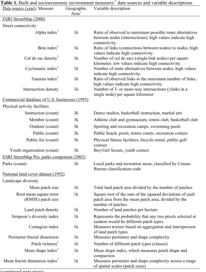
As described in the previous section, we analyzed environment variables calculated within buffers or census geographies selected based on preliminary analysis. Detailed descriptions and data sources of the following environment variables are presented in Section IV, Table 1.

Physical activity facilities/resources were obtained from a commercially purchased

time-varying national dataset containing street addresses and 8-digit Standard Industrial Classification codes (SIC). The database was validated against a field-based census of recreational facilities and resources, and demonstrated high overall agreement between commercial and field data in an urban and non-urban setting. Moreover, the patterns of error observed in the commercial data suggested that estimates of environment-health outcomes would not be substantially altered (125). Youth

organizations are comprised primarily of YMCA’s; due to the virtual duplication in these variables, YMCA’s were excluded from analysis. All analyses used unweighted counts of facilities within 3k buffers.

Local parks and recreation areas <200 acres were hypothesized to more strongly influence

routine activities than regional or national parks. Counts of local parks within 3k of each respondent residence were extracted from the parks component of ESRI StreetMap Pro. This data source has not been validated, and there is evidence that electronic sources of parks do not capture all parks;

however, these data provide comparable parks information in our nationally representative population.

(41)

Land cover data were derived from the software package Fragstats (126) based on the

national land cover dataset. Total area, mean patch size, patch count, and patch density were available for each of six land pattern classes: (1) water or perennial ice, (2) low & medium density developed, (3) high density developed, (4) recreational developed, (5) undeveloped/natural, and (6) agricultural. Fractal dimension indices and patch density of recreational and undeveloped land cover were also included in analysis.

Measures of the socioeconomic environment included the following: neighborhood sociodemographics included median household income (1990 measures inflated to 2000 dollars);

proportion of households below poverty and owning (versus renting) their homes; proportion of persons with at least a college education, of minority race/ethnicity was determined from the 1990 and 2000 U.S. Census. Non-violent and violent crimes per 100,000 population was assessed from Uniform Crime Reporting data, which reports county-level measures.

Physical activity (outcome)

Physical activity was the outcome of interest for this study because we hypothesize that it is

the outcome most directly related to the built environment. Add Health interviews employed a standard activity recall that elicited weekly frequency (bouts) of the following activities. (1) working around the house, such as cleaning, cooking, laundry, yardwork, or caring for a pet; (2) hobbies, such

as collecting baseball cards, playing a musical instrument, reading, or doing arts and crafts; (3) sedentary activities, such as watching television or videos, or play video games; (4) roller-blading,

roller skating, skate-boarding, or bicycling; (5) playing an active sport, such as baseball, softball,

(42)

28

questionnaires that were validated in other large-scale epidemiologic studies with regard to physical activity (127, 128).

Individuallevel covariates

Multivariate analyses analyzing physical activity as an outcome adjusted for the following individual-level characteristics: Race/ethnicity was self-reported at baseline (Wave I): respondents were classified as white, black, Asian, Native American, or Hispanic based on adolescent self-report and parental report. Age was calculated based on self-reported date of birth and interviewer-recorded interview date. Sex was self-reported at each study period and was used as a stratification variable or examined as a potential effect modifier due to known sex differences in determinants of physical activity. Socioeconomic position in young adulthood can be characterized by a complex array of behaviors and achievements (129, 130) which are likely predictors of residential relocation, so we used parent-reported household income and highest education attained to indicate socioeconomic position in both waves.

C. Sample

weights

and

survey

clustering

While multi-level (hierarchical) modeling has been encouraged for examining neighborhood effects on health (131), these methods are most appropriately applied to administrative or other boundary-defined neighborhoods. This project used buffer-defined built environment measures, which are individual-level exposures.

While census tracts and counties could be considered additional levels for neighborhood-level sociodemographic variables, they are not nested within schools, the primary sampling unit and

(43)

(44)

IV. Built

and

socioeconomic

environments:

patterning

and

associations

with

physical

activity

in

U.S.

adolescents

A. Abstract

Inter-relationships among built and socioeconomic environmental characteristics may result in confounding of associations between environment exposure measures and health behaviors or outcomes, but traditional multivariate adjustment can be inappropriate due to collinearity.

We used principle factor analysis to describe inter-relationships between a large set of geographic information system-derived built and socioeconomic environment measures for

adolescents in the National Longitudinal Study of Adolescent Health (Add Health; Wave I, 1995-96, n=17,441). Using resulting factors in sex-stratified multivariate negative binomial regression models, we tested for confounding of associations between various built and socioeconomic environment characteristics and moderate to vigorous physical activity (MVPA). Finally, we used knowledge gained from factor analysis to construct replicable environmental measures that account for inter-relationships and avoid collinearity.

(45)

household income, and crime rate) representing each environmental construct replicated associations with MVPA.

In conclusion, environmental characteristics are inter-related, and both the built and SES environments should be incorporated into analysis in order to minimize confounding. Single environmental measures may be useful proxies for environmental constructs in longitudinal analysis and replication in external populations, but more research is needed to better understand mechanisms of action, and ultimately identify policy-relevant environment characteristics with causal influence on physical activity.

B. Introduction

Numerous aspects of the built environment such as physical activity facilities (e.g., parks, recreation centers) (34, 133), “walkability” (76, 134), and neighborhood socioeconomic status (SES) (38, 135, 136) are related to physical activity and other key health behaviors and outcomes (37, 137, 138). However, built and SES environments are theoretically and empirically correlated; for example, physical activity facilities are more common in wealthier neighborhoods (33) and streets may be more connected in the poor inner-city (139). Therefore, neighborhood health studies that examine single or narrow sets of environmental characteristics are vulnerable to confounding by other environmental variables.

While strong correlations between environmental measures raise concerns about potential confounding, they also preclude extensive covariate adjustment due to collinearity. Pattern analysis techniques, such as factor analysis, are a common strategy for overcoming collinearity and accounting for the potentially interactive effects of environmental characteristics (105, 139-142). However, because the resulting factors are data-driven and population specific, analyzing the resulting factors longitudinally or in external populations is not straightforward. Finally, while replicable

(46)

32

activity facilities (33, 34). Further, most work has been in constrained geographic areas (30) or large geographic units such as counties (63).

Using nationally representative data on U.S. adolescents, a group at risk for dramatic declines in physical activity (50, 51), we sought to (1) describe inter-relationships between a large set of built and SES environment measures in a nationally representative sample of adolescents, (2) quantify the extent to which inter-related environment measures confound associations with moderate to vigorous physical activity (MVPA), and (3) demonstrate a strategy for using pattern analysis results to

construct replicable environmental measures that accounts for inter-relationships and avoids collinearity. While this study is largely exploratory, we hypothesized that (1) inter-relationships between and among built and SES environment measures would be substantial, (2) both built and SES environment measures would confound built environment associations with MVPA, and (3) indicator measures with the largest loadings in exploratory factor analysis (EFA) would adequately represent each environment factor.

C. Methods

Study population and data sources

We used cross-sectional Wave I data from The National Longitudinal Study of Adolescent Health (Add Health), a cohort study of 20,745 adolescents representative of the U.S. school-based population in grades 7 to 12 (11-22 years of age) in 1994-95. Add Health included a core sample plus subsamples of selected minority and other groupings collected under protocols approved by the Institutional Review Board at the University of North Carolina at Chapel Hill. The survey design and sampling frame are described elsewhere (143).

Neighborhood-level variables were created using a geographic information system (GIS) that links community-level data to Add Health respondent residential locations in space and time.

(47)

(n=15,480), (2) global positioning system (GPS) measurements (n=2,996), (3) ZIP/ZIP+4/ZIP+2 centroid match (n=205), (4) respondent’s geocoded school location (n=243). Individual-level and environmental measures differed for respondents located with GPS compared to other sources, reflecting rural locations in which Post Office Boxes or other addresses that cannot be geocoded. Otherwise, individual-level and environmental measures were similar across residential location source. Residential locations were linked to attributes of the circular area within 1, 3, 5, and 8.05 kilometers (k) of each respondent residence (Euclidean neighborhood buffer) and block group, tract, and county attributes from U.S. Census and other federal sources, which were merged with

individual-level Add Health interview responses.

To facilitate national representation of adolescent neighborhood environments, missing environmental data (n=463, 2.4%) was the only exclusion criterion for environmental patterning analyses, resulting in 18,461 adolescents. In estimation of associations with MVPA, exclusions included self-reported pregnancy (n=401) or mobility disability (n=122) and Native Americans due to small sample size (n=156); of the remaining sample (18,248), those with missing analytic variables (n=366 missing individual-level variables, 433 missing environmental variables, 8 missing both) were also excluded for an analytical sample of 17,441 adolescents.

Study variables

GISderived environmental characteristics

We examined built and SES environment measures with conceptual relevance or evidence of physical activity relationships in existing literature; see Table 1 for variable definitions and data sources and additional details below. While our environmental variables were created within various

neighborhood buffers or Census geographies, we used neighborhoods (e.g., 1 or 3k buffer, or Census tracts) consistent with the strongest associations with MVPA in previous analysis (74).

PA facility counts were obtained from a commercial dataset of U.S. businesses validated

(48)

34

high overall agreement between commercial and field data (125). Facilities were classified according to 8-digit Standard Industrial Classification (SIC) codes into overlapping types (Table 1). Several measures of landscape diversity and complexity (144) were created by analyzing national land cover data using the software package Fragstats (126). We examined several measures of street

connectivity calculated based on classical graph theory (145). High street connectivity provides

numerous route options and is characterized by dense, parallel routes, many intersections, and few cul de sacs and dead end streets (11). Census population counts within 1k buffers were calculated as averages weighted according to the proportion of the block-group area captured within 1k, then divided by the buffer area to obtain population density.

SES environment measures included economic (median household income and proportion of persons below poverty, college degree or greater) and social (proportion minority race/ethnicity, and owning their homes; crime rate) environment characteristics.

Individuallevel selfreported behaviors and sociodemographics

Weekly frequency (bouts) of MVPA (skating & cycling, exercise, and active sports) was ascertained using a standard, interview administered activity recall based on questionnaires validated in other epidemiologic studies (146).

Individual-level sociodemographic control variables included age at Wave I interview, self-identified race (white, black, Asian, Hispanic), parent-reported annual household income and highest level of education (<high school, high school or GED, some college, ≥college degree), and

administratively determined U.S. region (West, Midwest, South, and Northeast). Distributions of these variables in the analytical sample are reported in Table 2.

Do active communities support activity, or support active people? : residential self-selection in the estimation of built environment influences on physical activity

Acknowledgements

Table

of

Contents

List

of

Tables

List

of

Figures

List

of

Abbreviations

A.

Background

B.

Research

Aims

II.

Literature Review

A.

Determinants of Physical Activity

B.

Research Gaps

C.

Conclusion

III.

Methods

A.

Study

Population

and

Data

Sources

B.

Analytical

Variables

C.

Sample

weights

and

survey

clustering

IV.

Built

and

socioeconomic

environments:

patterning

and

associations

with

physical

activity

in

U.S.

adolescents

A.

Abstract

B.

Introduction

C.

Methods