High Dimension, Low Sample Size Data Analysis
Jeongyoun Ahn
A dissertation submitted to the faculty of the University of North Carolina at Chapel Hill in partial fulfillment of the requirements for the degree of Doctor of Philosophy in the Department of Statistics and Operations Research.
Chapel Hill 2006
Approved by Advisor: Dr. J. S. Marron Reader: Dr. Keith E. Muller
ABSTRACT
JEONGYOUN AHN: High Dimension, Low Sample Size Data Analysis (Under the direction of Dr. J. S. Marron)
This dissertation consists of three research topics regarding High Dimension, Low Sample Size (HDLSS) data analysis. The first topic is a study of the sample covariance matrix of a data set with extremely large dimensionality, but with relatively small sample size. Especially the asymptotic behavior of eigenvalues and eigenvectors of the sample covariance matrix is the focus of our study. Assuming that the true population covariance matrix of the data is not too far from identity matrix (i.e., spherical in the Gaussian case), we show that the sample eigenvalues and eigenvectors tend to behave as if the true structure of the data is indeed from identity covariance. Based on this, the asymptotic geometric representation of HDLSS data is extended to a wide range of underlying distributions. The representation essentially states that data vectors form a regular simplex in the data space with the number of vertices equal to the sample size.
The second part of the dissertation studies a discriminant direction vector, which is only interesting in HDLSS settings. This direction is characterized by the property that it projects all the data vectors, which are generated from two classes, to two distinct values, one for each class. It will be seen that this Maximal Data Piling (MDP) direction lies within the hyperplane generated by all the data vectors, while it is orthogonal to the hyperplanes generated by each class. It has the largest distance between piling sites among all the possible piling direction vectors and also maximizes the amount of piling. The formula of MDP is equivalent to the Fisher’s linear discrimination when the dimension is less than the sample size. As a classification method, MDP is heuristically desirable when the data are well approximated by the HDLSS geometric representation.
ACKNOWLEDGMENTS
This dissertation has been made possible by many people who have supported me. First of all I am very grateful to my advisor Steve Marron who guided this work with many fruitful, insightful discussions. He gave me the chance to participate in several interesting research groups and their research projects.
I would like to express my sincere thanks to Helen Hao Zhang, Keith E. Muller and Yufeng Liu for the opportunities of great collaborations and also their support in the dissertation work. The research assistantship with Harry Hurd in UNC hospitals and Cystic Fibrosis center was an invaluable experience working outside the department.
CONTENTS
List of Figures vi
List of Tables viii
1 Introduction 1
2 HDLSS Asymptotics:
Sample Covariance Matrices and the Geometric Representation 4
2.1 Introduction . . . 4
2.2 (d, n)-Asymptotics of Sample Covariance Matrices . . . 6
2.2.1 Hypothesis Tests for the Population Covariance Matrix . . . 6
2.2.2 Spectral Distribution of Sample Covariance Matrices . . . 8
2.2.3 Sample Eigenvalues from the Spherical Distribution . . . 10
2.2.4 Sample Eigenvalues from the Spiked Population Model . . . 12
2.3 d-Asymptotic Properties of Sample Covariance Matrices . . . 15
2.4 An Extremely Spiked Population Model . . . 20
2.4.1 The First Sample Eigenvalue . . . 20
2.4.2 The First Sample Eigenvector . . . 21
2.5 HDLSS Geometric Representation . . . 23
3 The Direction of Maximal Data Piling in High Dimensional Spaces 27 3.1 Introduction to Linear Discrimination . . . 27
3.1.1 Mean Difference . . . 29
3.1.2 Fisher’s Linear Discrimination . . . 30
3.1.4 Distance Weighted Discrimination . . . 33
3.2 The MDP Direction Vector . . . 34
3.2.1 Introduction to MDP . . . 34
3.2.2 A Toy Data Example . . . 36
3.3 Mathematics of the MDP Direction . . . 38
3.3.1 Characterization of the MDP Direction Vector in the Data Space . . . 38
3.3.2 Relationship to Fisher’s Linear Discrimination . . . 45
3.4 MDP as a Linear Classifier . . . 49
3.4.1 Relationship to the Support Vector Machine . . . 49
3.4.2 Gene Expression Data Example . . . 52
3.4.3 A HDLSS Comparative Simulation Study . . . 54
4 Bandwidth Selection for Kernel Based Classification 57 4.1 Introduction to the Kernel Based Classification . . . 57
4.1.1 Kernel Function . . . 59
4.1.2 Examples . . . 61
4.1.3 Gaussian Kernel and the Infinite Dimensional Feature Space . . . 63
4.2 Current Approaches to Bandwidth Selection . . . 67
4.2.1 Asymptotics of the Bandwidth Parameter . . . 67
4.2.2 Existing Tuning Methods . . . 69
4.3 Some Ideas from Kernel Density Estimation . . . 71
4.3.1 Maximal Smoothing Bandwidth Idea from Kernel Density Estimation . . 71
4.3.2 Scale-space Approach . . . 74
4.4 New Approach . . . 76
4.4.1 Motivation . . . 76
4.4.2 Data Examples . . . 78
LIST OF FIGURES
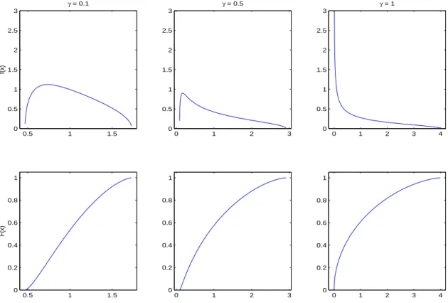
2.1 The density and distribution functions of the Marˇcenko-Pastur distribution. . . . 9 2.2 The density and distribution function of the Tracy-Widom distribution G1. . . . 11
3.1 Separable toy data in R2, with a separating hyperplane, shown as the dashed
line, and projections (dotted lines) onto the normal vector (solid line). . . 29 3.2 Visualization of a toy HDLSS data based on 1 and 2 dimensional projections
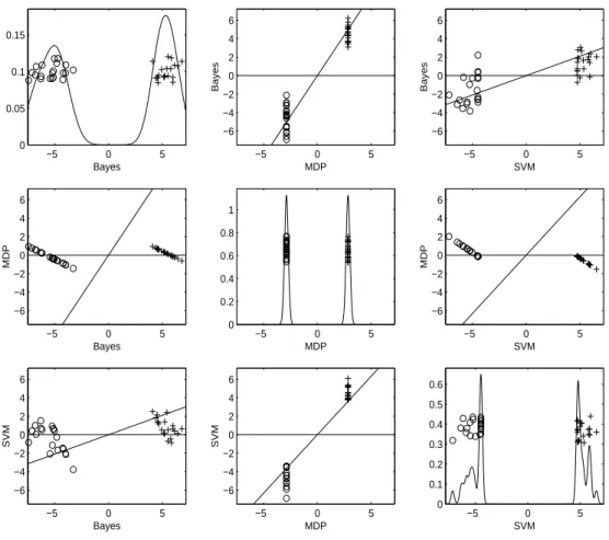
(d= 4000,n= 60). The three projection directions, used in the diagonal panels, are the first coordinate direction, the MDP direction, and the first principal component direction. The off-diagonal panels show the projected data on the plane generated by the respective two directions. . . 37 3.3 The illustration ofHX,HY, and vMDP when n1= 2,and n2 = 2. . . 42
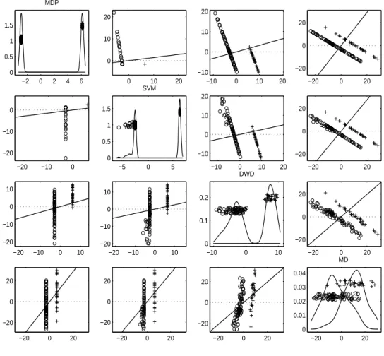
3.4 Illustration of data piling for the SVM and the MDP direction using a toy data example (d = 50, n = 40). Here the three projection directions are the the-oretically optimal Bayes rule, the MDP, and the SVM direction. Shows none, complete, and moderate data piling respectively. . . 51 3.5 Projections of microarray data onto MDP, SVM, DWD, and MD direction
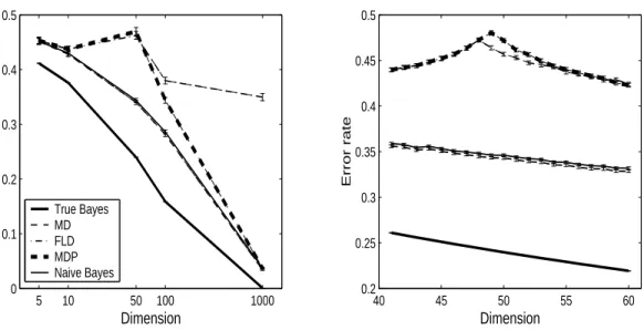
vec-tors, with 1-dprojections onto each direction vectors on the diagonal panels and 2-dprojections onto the plane generated by each pair of the direction vectors on the off-diagonal panels . . . 53 3.6 Misclassification error rate shown with error bars for the Bayes, MD, FLD, MDP,
and Naive Bayes method from the simulation withn= 50. Left hand panels are for d = (5,10,50,100,1000) with 100 repetitions and right hand panels are for d= (41,· · ·,60) with 1000 repetitions. . . 55
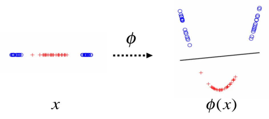
4.1 An illustration of data embedding. The data inR1 (left) becomes linearly
4.3 Two dimensional MDS representations of the target toy data in the feature space generated by the Gaussian kernels with different choices of the bandwidths. . . . 66 4.4 SVM classification result on target-shaped toy example with different
combina-tions of h and C . . . 68 4.5 Kernel MD Classification result of the maximal smoothing bandwidth hMS for
target-shaped toy example, shown with a range of h . . . 72 4.6 Pairwise distances in the feature space and the maximal smoothing bandwidth
hMS. The ‘+’ symbol and ‘o’ are used for Class +1 and Class−1, respectively.
The within pairwise distances of Class +1 (−1) are shown in the top (middle) jit-tered layer and their kernel density estimates are shown with the dotted (dashed) curve. The between class pairwise distances are shown as the x’s in the bottom jittered layer and the kernel density estimate is shown with the solid curve. The maximal smoothing bandwidthhMS= 0.68 is shown with the vertical line. . . 73
4.7 Training error of kernel MD over a range ofh, for target-shaped data and point cloud data. Data are shown in the top panels and the training errors are shown in the bottom panels. . . 75 4.8 Values of Dfor target toy example over a range of bandwidthh . . . 77 4.9 Boxplots of test errors, computing time, and selected bandwidth of kernel MD
for three data sets. . . 79 4.10 Boxplots of test errors, computing time, and selected bandwidth of kernel SVM
LIST OF TABLES
CHAPTER 1
Introduction
Data sets with more variables (i.e., attributes or entries in the data vector) than observations are now important in many fields. For example, in genetics a typical microarray gene expression data set has the number of genes ranging from thousands to tens of thousands, while the number of tissue samples (i.e., observations) is less than several hundreds (see for example Golubet al.
(1999) and Furey et al. (2000)). Data from medical imaging, and from text recognition also often have a much larger dimensiondthan the sample sizen. The term “High Dimension Low Sample Size (HDLSS)” will be used for this type of situation in this dissertation. Other terms such as “large p small n” (from the usage of p for the number of variables), appear in other references such as Bickel and Levina (2004). We view these as synonyms. As the technologies for collecting information are improving, it is quite likely that one will face HDLSS data more frequently in future applications.
the whole covariance. Chapter 2 and 3 discuss this topic in detail.
Several methods have been developed which confront the HDLSS challenge. Methods that reduce a high dimension to a lower, more manageable dimension have been developed over a number of years. For example, the dimension reduction techniques based on principal component analysis (PCA) find a set of new variables explaining most of the variability in the data. The number of these principal components can be as large as n−1, but usually one expects it to be much smaller than n or d, in practice. Feature selection or variable selection methods find a subset of variables that are most relevant to the objective of analysis. In supervised learning problems such as regression or classification, a popular solution to the model unidentifiability problem caused by the singularity of the covariance, is to put a restriction on the model space. For example, a smoothing constraint on coefficients can be added to the objective function (Hastie and Tibshirani, 2004).
Most methods discussed above were originally developed under the assumption of d < n. They have been applied to the HDLSS cases because it is plausible and seems appropriate. However, they do not consider the characteristics of HDLSS data which are quite different from typical non-HDLSS data. Especially HDLSS data are known to have some surprising and often counter-intuitive geometrical structure (Hall et al., 2005). For example, mean zero Gaussian random samples in a very high dimensional space are hardly present near the population mean. Not only that, they also tend to be farther away from the origin as the dimension increases, which appears paradoxical since the Gaussian density is largest near the origin. More detailed discussion of this topic can be found in Chapter 2.
This dissertation takes geometrical approaches to several statistical problems regarding HDLSS data analysis. Each of the problems is introduced along with a literature review and discussed in detail in separate chapters.
In Chapter 2, a non-classical type of asymptotics of the sample covariance matrix from HDLSS data is studied. Some of the results imply a shortcoming of PCA applied in HDLSS settings. Also, the asymptotical geometric representation of HDLSS data, which was first introduced in Hallet al.(2005), is established under much milder assumptions than the original work.
The binary discrimination problem in HDLSS settings is considered in Chapter 3. In particular a phenomenon called “data piling” (Marron et al., 2005) is explored. A direction vector in the data space that maximizes data piling is the main topic of the chapter and is discussed with a careful mathematical treatment and geometrical characterization. Also this direction is compared with some other popular discriminant directions as a linear classification method.
CHAPTER 2
HDLSS Asymptotics:
Sample Covariance Matrices and the Geometric Representation
2.1 Introduction
Asymptotic studies regarding HDLSS data are of increasing interest to many researchers. While the classical asymptotic analysis deals with the sample size increasing with fixed dimen-sionality, an important type of asymptotics, which is more relevant for HDLSS data, studies the case where the dimensiond increases. Sample sizencan grow with dat the same rate or it can be fixed. We will use notations such as n-, (d, n), and d-asymptotics to denote these three different kinds of asymptotics: The traditional large sample asymptotics will be denoted by n-asymptotics, the asymptotics for both simultaneously increasing dimension and sample size will be denoted by (d, n)-asymptotics, and finally the asymptotics for increasing dimension with a fixed sample size will be denoted by d-asymptotics.
Unlike the aforementioned works, Hall et al. (2005) let only d tend to infinity, i.e., take a d-asymptotic approach. They examine the geometry of HDLSS data and showed that under some conditions on the underlying distribution, pairwise distances between the data vectors become a constant as dgrows with a fixed n. This geometric representation essentially means that the randomness of data, with an extremely high dimensionality and small sample size, only lies in random rotations of a regular n-simplex in Rd. (See Section 2.5 for details.) In
their paper, they applied this to the binary classification problem and obtained some insights about asymptotic behaviors of some popular discrimination methods such as the support vector machines (Section 3.1.3) and the distance weighted discrimination (Section 3.1.4).
The original work of Hallet al.(2005) requires the variables to be “nearly independent” and the condition they imposed views the data entries (variables) as a time series. This assumption has some evident shortcomings. First, it is somewhat too strict because it is common to have a severe collinearity among variables. Second, the condition also depends on the order of the data entries, which can be arbitrary.
In this chapter, d-asymptotic properties of the sample covariance matrix are studied in Section 2.3. From this result, it is shown that the geometric representation in Hallet al.(2005) can be extended to a much more general condition in Section 2.5. The new condition is on the population eigenvalues and controls the departure from sphericity by restricting the relative size of dominating eigenvalues.
In the (d, n)-asymptotic limit, it is known that eigenvalues of the sample covariance matrix behave as if the underlying covariance were identity, which is the so-called “phase transition” phenomenon. The sufficient condition for this is that the underlying structure of the data is not far from spherical in the sense that non-unit eigenvalues are not much larger than one ( Section 2.2.4). Paul (2005) shows that sample eigenvectors also undergo the same phenomenon. It turns out that this also happens in the d-asymptotic case in Section 2.3.
eigenvalue still fails to converge to its population counterpart. This model can be considered as an extreme case of the “spiked population model” (Section 2.2.4).
2.2 (d, n)-Asymptotics of Sample Covariance Matrices
Assume a d×n data matrix X is from the multivariate Gaussian distribution with mean zero and covariance Σ, i.e., each d-length column vector, xj,j = 1,· · ·, n, are independently
and identically distributed as Nd(0,Σ). Denote the sample covariance matrix by S:
S= 1 nXX
T
. (2.1)
Note that the sample mean is not subtracted from the data matrix in (2.1). S is easier to handle than the usual sample covariance matrix with mean subtracted in this setting. Also it is the maximum likelihood estimator of Σ. In the following subsections, various topics involving S when the dimension/sample size ratio d/n approaches some constant γ ∈ (0,∞) as d increases, are reviewed. During most of those discussions, even though the entries of the matrix X depends on both d and n, we suppress the indices for the sake of simplicity of notation.
2.2.1 Hypothesis Tests for the Population Covariance Matrix
In this section, two common hypothesis testing problems, for the sample covariance matrix from the Gaussian distribution, are considered.
The first testing problem is whether the underlying distribution is spherical. The testing hypotheses of the sphericity test are
H0 :Σ=σ2I vs. H1:Σ6=σ2I, (2.2)
whereσ is not specified. The likelihood ratio criterion by Mauchly (1940) is
R1=
|A|12n
(tr(A)/d)12dn
,
The locally most powerful test for (2.2) is based on the statistic (John, 1971)
U = 1 dtr
"
S tr(S)/d−I
2#
, (2.3)
and U is well-defined even whend > n.
The second hypothesis testing problem is to test whether the underlying covariance is equal to a given positive definite matrixΣ0. This is equivalent to testing
H0 :Σ=I vs. H1:Σ6=I,
by multiplying the data byΣ−01/2. The likelihood ratio criterion (Anderson, 2003, Chapter 10) is
R2 = e
n
12dn
|A|12ne− 1 2tr(A),
which is also degenerate when d > n. A non-degenerate testing criterion (Nagao, 1973), well defined even if the dimensionality exceeds the sample size, is
V = 1 dtr
(S−I)2,
which can be derived in a similar way asU for the test ofΣ=I.
Ledoit and Wolf (2002) studied asymptotic behaviors of the tests based on U and V, as d andngo to infinity together with the ratiod/nconverging to a limitγ ∈(0,∞). They showed that the sphericity test based on the test statisticU remains consistent asd/n→γ, in the sense that the (d, n)-asymptotic limiting distribution of U is the same as its n-asymptotic limiting distribution. However, it no longer holds for the second type of test based onV.
Ledoit and Wolf (2002) modified V and introduced a new test statistic W as follows:
W = 1 dtr
(S−I)2
− d n
tr(S) d
2
+ d n.
i.e., is not only consistent in then-asymptotic sense, but also itsn-asymptotic properties remain valid in the limit ofd/n→γ. Birke and Dette (2003) investigated (d, n)-asymptotic properties of U,V, and W when the ratiod/ngoes to either zero or infinity.
2.2.2 Spectral Distribution of Sample Covariance Matrices
Let `1 > · · · > `d be the eigenvalues of a sample covariance matrix S from the spherical
Gaussian distribution, i.e., fromNd(0,I). The empirical distribution of these sample
eigenval-ues is called the empirical spectral distribution of S, and defined by
Fd(x) =
1
d×number of elements in{i:`i 6x}.
The limiting spectral distribution, i.e., the limit of Fd, if d/n goes to γ ∈ (0,1] as d → ∞,
was first obtained by Marˇcenko and Pastur (1967). Fd converges to the Marˇcenko-Pastur
distributionF, defined with the density function
f(x) =F0(x) =
(2πγx)−1p(x−a)(b−x) a < x < b
0 otherwise,
(2.4)
wherea= (1−√γ)2 andb= (1 +√γ)2. Whenγ >1, this distribution has an additional Dirac measure at x= 0 of mass 1−1
c.
The survey paper by Bai (1999) has a comprehensive review on the spectral distribution, for both the real and the complex cases. Under some conditions on moments, Bai et al.
(2003) found out that the order of the convergence in (2.4) is Op(n−2/5) when γ is not close
to 1 in the sense that γ < 1−O(n−1/8), and Op(n−1/8) when γ is close to 1 in the sense
that γ > 1−O(n−1/8). The model with Σ that has a few non-unit eigenvalues is called the
“spiked population model” (Section 2.2.4). It is known (Silverstein and Bai, 1995) that the Marˇchenko-Pastur limit still holds for this case too, with possibly different support depending on the model.
0.5 1 1.5 0 0.5 1 1.5 2 2.5 3
γ = 0.1
f(x)
0 1 2 3 4
0 0.2 0.4 0.6 0.8 1
0 1 2 3
0 0.5 1 1.5 2 2.5 3
γ = 0.5
0.5 1 1.5
0 0.2 0.4 0.6 0.8 1 F(x)
0 1 2 3
0 0.2 0.4 0.6 0.8 1
0 1 2 3 4
0 0.5 1 1.5 2 2.5 3
γ = 1
Figure 2.1: The density and distribution functions of the Marˇcenko-Pastur distribution.
skewed than the densities for smaller γ’s, with more mass around zero.
Note that this limiting spectral distribution is useful in obtaining the asymptotic behavior of a function of the form
Tn ≡
1
d{φ(`1) +· · ·+φ(`d)} =
Z ∞
0
φ(x)dFd(x),
since it converges to
Z ∞
0
φ(x)dF(x),
2.2.3 Sample Eigenvalues from the Spherical Distribution
While the results in the previous section are about the whole bulk of the sample eigenvalues, in this and the following sections we consider asymptotic properties of each eigenvalue. The identity covariance matrix is considered here and the non-identity case is considered in the next section.
Geman (1980) showed that, for a spherical Gaussian distribution, the largest sample eigen-value converges to the upper edge of the support ofF in (2.4):
`1 →(1 +
√
γ)2 almost surely. (2.5)
An analogous result for the smallest eigenvalue holds (Silverstein, 1985; Bai and Yin, 1993):
`min{d,n}→(1−√γ)2 almost surely, (2.6)
i.e., it converges to the lower edge of the support. Yinet al.(1988) generalized these results to non-Gaussian cases under the assumption of a finite fourth moment. Note that these results do not provide any information on the variability, or the distribution of the largest or the smallest eigenvalues.
For the Gaussian case, the limiting distribution of the largest sample eigenvalue`1 is derived
by Johnstone (2001). If we define the center and scaling constants as follows:
µnd = (
√
n−1 + √
d)2, (2.7)
σnd = (
√
n−1 +√d)
1 √
n−1 + 1 √ d
1/3
, (2.8)
then asd/n→γ ∈(0,1],
n`1−µnd
σnd D
−→W1∼G1. (2.9)
The limiting distribution function G1 is defined by
G1(s) = exp
−1 2
Z ∞
q(x) + (x−s)q2(x) dx
−5 0 5 0
0.01 0.02
g
1(s)
−5 0 5
0 0.5 1
G
1(s)
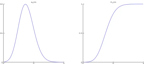
Figure 2.2: The density and distribution function of the Tracy-Widom distribution G1.
whereq(x) solves the Painlev`e II differential equation
q00(x) = xq(x) + 2q3(x), q(x) ∼ Ai(x) as x→ ∞,
and Ai(x) denotes the Airy function (Deift, 1999). Tracy and Widom (1996) first found this distribution as the limiting law of the largest eigenvalue of an n by n Gaussian symmetric matrix. Note that the mean constant (2.7) divided by ngives (√1−n−1+p
d/n)2, which is about the same as the limit (2.5) except for a slight adjustment to the quality of approximation for small n.
The distributionGhas been numerically evaluated (Pr¨ahofer and Spohn, 2003) and plotted in Figure 2.2. It is asymmetric, has mean =. −1.21 and standard deviation = 1.27 and decays. like exp(−1
24|s|
3) at the left tail and exp(−2 3s
3/2) at the right. Comparing percentiles of the
empirical distribution of the largest sample eigenvalue and its limiting distribution, Johnstone (2001) argued that this approximation is reasonable for bothn anddas small as 5.
e
X = [˜x1,· · ·,x˜p]T where ˜xj =rjkxxjjk and rj is iid
1 nχ
2
n. Now the above approximation holds
for the largest eigenvalue of 1nXeXeT.
2.2.4 Sample Eigenvalues from the Spiked Population Model
The assumption of identity covariance is sometimes unrealistic since there are many cases where a few sample eigenvalues are separated from the rest of the eigenvalues. Such exam-ples include speech recognition (Johnstone, 2001; Buja et al., 1995), wireless communication (Telatar, 1999), and statistical learning (Hoyle and Rattray, 2004). In this section the spiked population model (Johnstone, 2001), where all but finitely many eigenvalues of the population covariance matrix are one, is considered as the underlying distribution.
Paul (2005) and Baik and Silverstein (2004) independently derived the almost sure limit of the largest sample eigenvalue from the spiked population model. The former work assumes the real Gaussian model, derives the asymptotic distribution of the largest eigenvalue, and also examines asymptotic properties of the corresponding eigenvector. Baik and Silverstein (2004) have a focus on the almost sure limits of the largest and the smallest eigenvalues in real/complex non-Gaussian cases.
Assume that the population distribution is Gaussian with mean zero and diagonal covariance matrix
Σ=diag(λ1,· · · , λ1, λ2,· · ·, λ2,· · ·, λM,· · ·, λM,1,· · ·,1),
where λ1 > · · · > λM > 0 with multiplicity k1,· · ·, kM, respectively. Set k0 = 0. Thus if
r=k1+· · ·kM, thend−rnumber of eigenvalues are one’s. Let us assume that`1 >· · ·>`d>0
are the sample eigenvalues and the ratiod/nconverges toγ asd, n→ ∞. Baik and Silverstein (2004) showed the following. Note that all the convergence results below are almost sure convergence.
(1) Case 0< γ <1.
Let M0 be the number of j’s such that λj >1 +
√
j’s such thatλj <1−
√
γ. Then, for each 16j 6M0,
`k1+···+kj−1+i→λj
1 + γ λj−1
, 16i6kj. (2.10)
For eachM1+ 16j6M,
`d−r+k1···+kj−1+i →λj
1 + γ λj−1
, 16i6kj. (2.11)
Also
`k1+···kM0+1 → (1 + √
γ)2, and (2.12)
`d−r+k1+···+kM1 → (1−
√
γ)2. (2.13)
Note that (2.10) is for the largestk1+· · ·+kM0 eigenvalues and (2.11) is for the smallest
kM1+1 +· · ·+kM eigenvalues. The results (2.10) and (2.12) are proved also by Paul
(2005). (2) Caseγ >1.
LetM0 be the number ofj’s such that λj >1 +
√
γ. Then, for each 16j 6M0,
`k1+···+kj−1+i→λj
1 + γ λj−1
, 16i6kj.
Also
`k1+···kM0+1 → (1 + √
γ)2,
`n → (1−
√
γ)2, and `n+1 =· · ·=`d = 0.
(3) Caseγ = 1.
LetM0 be the number ofj’s such that λj >2. Then for each 16j6M0,
`k1+···+kj−1+i→λj
1 + γ λ −1
Also
`k1+···kM0+1 → 4, and `min{n,d} → 0.
The overlapping results of Baik and Silverstein (2004) and Paul (2005) say that if the population eigenvalue λj is larger than 1 +
√
γ then the corresponding sample eigenvalue `j converges to
λj
1 +λγ j−1
almost surely, and if λj is less than 1 +
√
γ then`j converges to (1 +
√ γ)2. Note that the limits in (2.12) and (2.13) are the same as the limits in (2.5) and(2.6). In other words, the limit of the largest (or smallest) eigenvalue from a non-identity underlying covariance is the same as the limit from the identity covariance. This “phase transition” phenomenon means that if the deviance from sphericity is not strong enough, in the sense that the largest true eigenvalue is less than 1 +√γ or the smallest one is bigger than 1−√γ, then the sample eigenvalue behaves as if it is from the identity covariance.
Now let us consider asymptotic distributions of sample eigenvalues. The (d, n)-asymptotic normality of the largest sample eigenvalue is shown by Paul (2005), in the case of a severe spiked Gaussian population model: Ifλj >1 +
√
γ with multiplicity one and nd−γ =o(n−1/2), then
√
n(`j−µj) D
−→N(0, σj2),
whereµj =λj
1 +λγ j−1
andσ2j = 2λ2j
1− (λ γ j−1)2
.
The phase transition phenomenon also happens in sample eigenvectors (Paul, 2005). Sup-pose thej-th population eigenvectorvj,j= 1,· · ·, disd×1 vector with 1 in thej-th coordinate
and zeros elsewhere and let ej be the corresponding sample eigenvector. Then the following
results hold whend/n→γ ∈(0,1):
(a) Ifλj 61 +
√ γ,
<ej,vj > a.s.
(b) Ifλj >1 +
√
γ and of multiplicity one, then
|<ej,vj >| a.s.
−−→
s
1− γ
(λj−1)2
/
1 + γ λj−1
as n, d→ ∞.
The inconsistency of principal component analysis in a high dimensional setting has been ob-served (Johnstone and Lu, 2004). The above result in (a) proves a stronger version of the inconsistency for the mildly spiked population model.
2.3 d-Asymptotic Properties of Sample Covariance Matrices
In this section we examine the asymptotic properties of the sample covariance matrix when only the dimension d tends to infinity while the sample size n is fixed, since the order of magnitude of dis much larger thann in many real data sets.
Suppose we have a d×n(d > n) data matrix
X≡[x1,· · · ,xn],
wherexj = (x1j,· · · , xdj)T are iid from a d-multivariate distribution with mean zero and
non-negative definite covariance matrix Σ. Note that [,] is for the horizontal concatenation of vectors/matrices. The eigenvalue decomposition of Σ is Σ= VΛVT, where Λ is a diagonal
matrix of eigenvaluesλ1>· · ·>λd>0 andV is the matrix of corresponding eigenvectors. A
“factor matrix”, which is essentially the square root ofΣ, is defined asF≡VΛ1/2, which gives Σ=FFT. Using the factor matrixF, we can write X=FZ where
Z=Λ−12VTX
is ad×nrandom data matrix from d-multivariate distribution with identity covariance matrix. Note that ifXis from the multivariate Gaussian distribution, the elements ofZare independent standard univariate normal variables.
Using the factor matrix F, the sample covariance matrixS is decomposed as
S≡ 1 nXX
T= 1
nFZZ
A “dual” approach switches the columns and rows of the data matrix, replacingXbyXT. The
n×ndual sample covariance matrix
SD ≡
1 nX
TX.
Note that SD has the same eigenvalues asS. If we writeX asFZ and use the fact thatVTV
is the identity matrix,
nSD = (ZTFT)(FZ)
= ZTΛZ
=
d
X
i=1
λiWi, (2.14)
where the n×nmatrix Wi =zTizi and zi’s, i= 1,· · · , d, are row vectors of the matrixZ. If
X is Gaussian,Wi’s are independently from Wishart distributionWn(1,In).
Remark. If a matrix A has the Wishart distribution Wm(ν,G), then A = Pνi=1zizTi, where
z1,· · ·,zν are random vectors with an iid m-dimensional multivariate Gaussian distribution
with mean 0 and covariance matrix G. See Muirhead (1982) or Anderson (2003) for more details on this distribution.
The main theorem in this chapter states that under mild conditions on the population eigenvalues, SD becomes a scaled identity matrix for very large d with a fixed n. Thus all
the eigenvalues of SD (also those of S) approximately are the same. In a sense, extreme
HDLSS data behave as if the underlying distribution were spherical. This means that the phase transition phenomenon, observed for (d, n)-asymptotics in Section 2.2.4 also happens for d-asymptotics.
The assumption for this theorem can be conveniently characterized by a well-known measure of sphericity (Mulleret al., 2005)
≡ tr
2(Σ)
dtr(Σ2)
=
Pd
j=1λj 2
dPd
i=1λ2j
The empirical version of (2.15)
ˆ = tr
2(S)
dtr(S2),
is a locally most powerful invariant test statistic of sphericity of multivariate Gaussian distri-butions (John, 1972). Note that test statistics (2.3) in Section 2.2.1 can be expressed as a function of ˆ:
U = 1−ˆ ˆ .
Also note that these inequalities always hold:
1
d 661.
Note that perfect sphericity of the distribution occurs only when = 1. Our key assumption concerns the other end of thespectrum, in particular, we need d1 for larged, in the sense that −1 =o(d). In other words, the underlying distribution needs to be not too close to the most singular case, where only the first eigenvalue is nonzero.
Theorem 2.3.1. For a fixedn, consider a sequence ofd×nrandom matrices X1,· · ·,Xd,· · · from multivariate distributions with dimension d, with zero means and covariance matrices
Σ1,· · · ,Σd,· · ·. Let λ1,d > · · · > λd,d be the eigenvalues of the covariance matrix Σd, and
SD,d be the corresponding dual sample covariance matrix. Suppose the eigenvalues of Σd are sufficiently diffused, in the sense that
1 d =
Pd j=1λ2j,d
Pd
j=1λj,d
2 →0 as d→ ∞. (2.16)
Then the sample eigenvalues behave as if they are those of the identity covariance in the sense
that
SD,d
Kd
where Kd= n1Pdj=1λj,d.
Proof. By (2.14), any diagonal element of nSD,d can be expressed as Pdj=1λj,dZj2 where the
Zj’s are iid from univariate distribution with unit variance. Define the relative eigenvalueseλj,d
as
e
λj,d ≡
λj,d
Pd
j=1λj,d
.
Then by Chebyshev’s inequality and the assumption (2.16), for anyτ >0,
Pr d X j=1 e
λj,dZj2−1
> τ 6
varPd
j=1eλj,dZj2
τ2
= 2
Pd
j=1eλ2j,d
τ2 →0 as d→ ∞.
Thus a diagonal elementPd
j=1eλj,dZj2 converges to 1 almost surely.
The off-diagonal elements of nSD,d can be expressed as
Pd
j=1λj,dZjZj0 where theZj’s and
theZj0 are independent.
Pr d X j=1 e
λj,dZjZj0
> τ 6 var Pd
j=1λej,dZjZj0
τ2
=
Pd
j=1λe2j,d
τ2 →0 as d→ ∞.
Thus an off-diagonal element converges to 0 almost surely.
The condition (2.16) holds for quite general settings, including the following.
(a) Constant: λ1,d =· · · =λd,d =C, where C is a constant. This is a spherical case where
all the eigenvalues are the same. Since,
Pd
j=1λ2j,d
Pd
j=1λj,d
2 =
dC2 (dC)2 =
1
d →0 as d→ ∞.
k < d, α < 1, C1, C2 > 0. The first k eigenvalues are moderately larger than the rest.
Since,
Pd
j=1λ2j,d
Pd
j=1λj,d
2 =
kC12d2α+ (d−k)C22 (kC1dα+ (d−k)C2)2
= O(d∨d
2α)
O(d2) →0 as d→ ∞.
(c) Polynomial: λj,d =j−β, j = 1,· · · , d, ∀β >0. The eigenvalues decrease in polynomial
order. Since,
Pd
j=1λ2j,d
Pd
j=1λj,d
2 = Pd
j=1j
−2β
(Pd
j=1j−β)2
= O(d
−2β+1)
O(d−2β+2) →0 as d→ ∞.
The cases where the condition (2.16) fails include the following.
(d) Fixed Block, Large: λ1,d = · · · = λk,d = C1dα, λk+1,d = · · · = λd,d = C2, where
k < d, α>1, C1, C2>0. The firstkeigenvalues are greatly larger than the rest. Since, Pd
j=1λ2j,d
Pd
j=1λj,d
2 =
kc21d2α+ (d−k)C22 (kC1dα+ (d−k)C2)2
→C1 as d→ ∞.
(e) Exponential: λj,d =γj, j = 1,· · · , d, ∀ 0< γ < 1. The eigenvalues decrease
exponen-tially. Since,
Pd
j=1λ2j,d
Pd
j=1λj,d
2 =
(1−γ)2(1−γ2d)
(1−γ2)(1−γd)2 →
1−γ
1 +γ as d→ ∞.
(f) Finite Support: λj,d =C, j = 1,· · ·, k, λk+1,d =· · ·=λd,d= 0, k < d, C >0. Only the
first keigenvalues are nonzero. Since,
Pd
j=1λ2j,d
Pd
j=1λj,d 2 =
1 k.
2.4 An Extremely Spiked Population Model
For high dimensional data, PCA often fails to estimate the true directions and the variances of principal components, due to the phase transition phenomenon as explained earlier. The condition (2.16) characterizes an underlying structure of the data, which makes the PCA fail in providing reasonable estimates. While this condition is quite mild, there are some distribution models that do not satisfy (2.16). In this section we consider such an extreme case of the spiked population model, in order to see if the PCA can work well under this model. Specifically, we will look at whether the first sample eigenvalue and eigenvector can estimate their population analogs.
We assume that the extremely spiked population models considered here are a sequence of Gaussian distributions, i.e.,Nd(0,Σd), d= 1,2,· · ·. The diagonal covariance matrix Σd has a
dominating first eigenvalue, i.e.,
Σd≡Λd≡diag(dα,1,· · ·,1), (2.17)
whereα >1. Also the eigenvectors ofΣdare assumed to bed-dimensional unit vectors. Thus
the first eigenvalue and eigenvector for this model are dα and (1,0,· · ·,0)T, respectively. In a
factor analysis context, this model corresponds to single common factor model with uniqueness diminishing as d → ∞. It also can be seen as a special case of example (d) in Section 2.3. Note that we already looked at the case where 0< α <1 in the example (b) in that section. 2.4.1 The First Sample Eigenvalue
Let`1,d >· · ·> `n,dbe nonzero eigenvalues of the sample covariance matrixS(orSD). By
(2.14), the dual sample covariance matrix
SD =
1 n
d
X
j=1
λjWj
= 1
n
dαW1+ d
X
j=2
Wj
whereWj’s are iid Wn(1,In). If we define
U ≡ W1,
V ≡
d
X
j=2
Wj,
then U ∼ Wn(1,In) and V ∼ Wn(d−1,In), independently. Here the subscript ,d is being
omitted for the sake of simplicity in notation. Dividing SD by dα gives
1 dαSD =
1 nU+
1
ndαV. (2.18)
U can be expressed as the outer product of a random vector from the Nn(0,In) distribution
with itself. Thus it has rank one and the only nonzero eigenvalue is the inner product of that random vector with itself, which is a χ2n random variable. Also as d becomes large, V approximates (d−1)In. Hence ifα > 1, (2.18) converges to n1U as d→ ∞, since the second
term nd1αV tends to 0.
The first sample eigenvalue `1,d is approximately distributed as n1dαχ2n when d is large.
This means for fixed sample size n, the first sample eigenvalue is the product of the true eigenvalue and a random quantity depending on the specific realization of data. However, with a reasonably large n, n1χ2n is expected to be close to 1 by the law of large numbers, which makes the first sample eigenvalue close to the population counterpart. Note that the other eigenvalues converge to 0 asdincreases since U has rank one.
2.4.2 The First Sample Eigenvector
Consider the eigenvalue decomposition of S=GLGT, where
G={gij :i, j= 1,· · ·, d}
is the matrix of corresponding eigenvectors, ej = (g1j,· · · , gdj)T, j = 1,· · ·, d, are the
eigen-vectors, and
Now writing Λd in (2.17) asΛ to simplify the notation, define a standardized version ofS as
e
S ≡ Λ−12SΛ− 1 2
= Λ−12GLGTΛ− 1
2. (2.19)
Using the fact that
S = 1
nFZZ
TFT
= 1
nΛ
1 2ZZTΛ
1 2,
we have
e
S = 1
nΛ
−1 2Λ
1 2ZZTΛ
1 2Λ−
1 2
= 1
nZZ
T
∼ 1
nWd(n,Id), (2.20)
where Zis ad×ndata matrix whose elements are iid from the standard univariate Gaussian distribution. Note that Se is independent of the underlying covariance matrix Σd and its
diagonal elements are independently distributed as 1nχ2n. Also by (2.19), the i-th diagonal entry ofSe is
˜ sii=
g2i1`1,d+· · ·+gin2 `n,d+ 0 +· · ·+ 0
λi,d
.
If we plug in the underlying eigenvalues, then
˜ s11 =
g211`1,d+· · ·+g12n`n,d
dα ,
˜
sjj = g2j1`1,d+· · ·+g2jn`n,d, j= 2,· · ·, d.
From the result of Section 2.4.1, for a larged,
˜ s11 ≈
[limd→∞g112 ]dαχ2n
˜ sjj ≈
[limd→∞gj21]dαχ2n
n , j= 2,· · · , d.
Since by (2.20) ˜sjj ∼ n1χ2n, j= 1,· · · , d,
g211 → 1 as d→ ∞,
gj21 → 0 as d→ ∞, j= 2,· · · , d.
Thus, under the identifiability restriction that the first component of the eigenvector must be positive, e1 → (1,0,· · ·,0)T, i.e., the first sample eigenvector converges to the population
counterpart as dincreases.
2.5 HDLSS Geometric Representation
Understanding the geometric structure of HDLSS data is a challenging task due to the limitation of visualizing the data. In fact it is known that they have quite different geometry from low dimensional data. In their (d, n)- asymptotic study on simplices in high dimensional space, Donoho and Tanner (2005) found out that the convex hull ofnGaussian data vectors in Rd“looks like a simplex” as the ratiod/nconverges toγ ∈(0,1), in the sense that all points are
on the boundary of the convex hull. Furthermore, depending on the value ofγ, all the pairwise line segments, triangles, quadrangles, etc., are also on the boundary of the convex hull. In this section we focus on the geometry of HDLSS data using thed-asymptotic approach, letting only dtend to infinity, while fixing n.
Supposezd= (z1,· · · , zd)Tis ad-dimensional random vector from the Gaussian distribution
with mean zero and identity covariance matrix. Since the sum of squared entries of zd has
Chi-square distribution with degrees of freedomd, it can be shown that
kzdk=d12 +Op(1).
two is
kz1,d−z2,dk= (2d)
1
2 +Op(1). (2.21)
Note that data vectors tend to have a deterministic distance apart. Also they are approximately perpendicular because the angle between them
ang(z1,d,z2,d) =
1
2π+Op(d
−1
2). (2.22)
Both equations (4.7) and (2.22) hold for nrandom vectorsz1,d,· · ·,zn,d. This implies that all
pairwise distances are approximately equal and all pairwise angles are approximately perpen-dicular.
Hall et al. (2005) extended the above argument to the non-Gaussian case. Suppose xd=
(x1,· · · , xd)T is a random vector from a d-dimensional multivariate distribution. Assume the
following:
(1) The fourth moments of the entries of the data vectors are uniformly bounded. (2) For a constantσ2,
1 d
d
X
j=1
var(xj)→σ2.
(3) Viewed as a time series, x1,· · · , xd,· · · is ρ-mixing for functions that are dominated by
quadratics. That is, fori, j= 1,· · · , dwith|i−j|>r,
sup
|i−j|>r
|E(xixj)|6ρ(r)→0 as r→ ∞. (2.23)
Ifx1,d,· · ·,xn,d are random vectors from the distribution satisfying the conditions above, then
the distance betweenxi,d andxj,d,i6=j, is approximately (2σ2d)
1
2, in the sense that
d−12kxi,d−xj,dk →(2σ2) 1
Thus after scaling by d−12, the data vectorsxi,d are asymptotically located at the vertices of a
regular n-simplex where all the edges are of length (2σ2)12.
Hall et al.(2005) applied the above result to the two sample case in the context of binary classification. They also obtained some insights about limiting behaviors of some popular discrimination methods such as the support vector machines (see for example Cristianini and Shawe-Taylor (2000)) and the distance weighted discrimination (Marronet al., 2005).
The condition (3) requires entries in the data vector (variables) to be nearly independent. If the entries are far from each other in their locations in the data vector, the correlation between them should diminish. This condition is somewhat too strict because it is common to have a severe collinearity among variables and the condition also depends on the order of the data entries, which can be arbitrary. In this section we establish the same HDLSS geometric representation using Theorem 2.3.1 and show that our assumption (2.16) is more general than that of Hallet al. (2005).
Let xj,d = (x1j,· · ·, xdj)T, j = 1,· · ·, n, be j-th column of the data matrix X, i.e., j-th
sample, from thed-dimensional multivariate distribution with mean zero and covariance matrix Σd. Suppose the eigenvalues ofΣdsatisfy the condition (2.16). The squared distance between
xi,d andxj,d is
kxi,d−xj,dk2 = d
X
k=1
(xki−xkj)2
=
d
X
i=1
x2ki+
d
X
i=1
x2kj−2
d
X
i=1
xkixkj. (2.24)
Note that the first two terms in (2.24) are thei-th andj-th diagonal entries ofnSD respectively.
Thus for a sufficiently large d, both terms become close to Pd
j=1λj by Theorem 2.3.1. Also
since the third term is the (i, j)-th entry ofnSD, it diminishes to zero as dgrows. Thus, for
sufficiently large d, the pairwise distances become approximately
kxi,d−xj,dk ≈
2
d
X
j=1
λj
1 2
.
1,· · · , d,
E[xixj]→0 as |i−j| → ∞. (2.25)
Note that
d
X
k=1
λk,d = d
X
k=1
E[x2k], and
d
X
k=1
λ2k,d = tr(Σ2d) =
d
X
i,j=1
E[xixj]2.
Then the left hand side of (2.16) becomes
Pd
j=1λ2j,d
Pd
j=1λj,d
2 = Pd
i,j=1E[xixj]2 Pd
i,j=1E[x2i]E[x2j]
= o(d
2)
O(d2) →0 as d→ ∞,
CHAPTER 3
The Direction of Maximal Data Piling in High Dimensional
Spaces
3.1 Introduction to Linear Discrimination
Suppose we are given two classes of objects. We are then faced with a new object with unknown class information, which we are to assign to one of the two classes. The given objects with the known classes are called training data. This binary discrimination problem can be formulated as follows. Assume we are given the training data
(x1, t1),· · · ,(xn, tn)∈ X × {±1}.
Here,xi are called inputs or patterns, the class variabletiare sometimes called targets or labels,
and X is called the feature space where the xi are taken from.
It is commonly assumed that X is d-dimensional Euclidean space Rd and x
i are
indepen-dently and identically distributed random vectors onRd. We call each dimension of the feature
space a feature or a variable. Whenever it is easier to convey a particular idea, we will use x for the input vectors with Class +1 and yfor Class −1.
A discriminating function, or a classifierf(x) is a real valued function of a new data vector x∈ Rd. We assign x according to the sign of f(x), i.e., if f(x)>0 (<0) then we classify it
to the Class +1 (−1). The process of obtaining such classifiers is called a classification rule. A possible measure to evaluate a classifierf(x) is the training error
[ error =
Pn
i=11(sign(f(xi))6=ti)
where 1(·) is the indicator function. That is, the relative frequency of the training data points which have a discrepancy between the label predicted by f(x) and its actual label. However, we want our classifier to work well eventually for future observations as well as the observations at hand, i.e., to have a good generalizability (Cristianini and Shawe-Taylor, 2000). Thus it is always desirable that we use the misclassification error evaluated from a separate test data set, i.e., the data independently generated from the same distribution as the training data. The misclassification error from the test data can be used to approximate the classification error, which is the expected relative frequency over all the possible test data sets. When the test data set is not available, the V-fold cross validation (Burman, 1989; Wahba et al., 2000) can approximate the test error. See Chapter 4 for more discussion of cross-validation.
Duda et al. (2000) gives broad reviews on various discrimination methods, also covering some recent topics in the context of machine learning. Standard textbooks on multivari-ate data analysis such as Mardia (1980) and Kachigan (1991) have discussions on traditional approaches for discriminant analysis, such as Fisher’s linear discrimination. For recently devel-oped classification algorithms such as CART, Hastieet al.(2001), Sch¨olkopf and Smola (2001), and Shawe-Taylor and Cristianini (2004) give good overviews of the many references that are available.
We call a classifier linear/nonlinear if the discriminating function f(x) is a linear/nonlinear function ofx. In this chapter only linear classifiers are considered. In the classification problem in a HDLSS setting, a linear classifier often gives better performance than most standard nonlinear classifier in many applications (Hastie et al., 2001, Chapter 5), even though the nonlinear classifier rules are generally more flexible (Chapter 4). We can explain this by the HDLSS asymptotics in Section 2.5, since the data vectors approximately form two simplices for each class, where a linear classifier can be a heuristically reasonable choice.
The classification boundary generated by a linear classifier is a linear separating hyperplane between the two classes. A linear classifier inRd can be expressed
f(x) =wT
x+b, (3.1)
Class +1
Class −1
Normal Vector
Separating Hyperplane
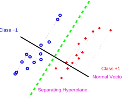
Figure 3.1: Separable toy data in R2, with a separating hyperplane, shown as the dashed line, and
projections (dotted lines) onto the normal vector (solid line).
b is called the bias or the shift parameter. Figure 3.1 shows a toy data set in R2 with a
separating hyperplane. It also shows the projections of the data points onto the normal vector of the hyperplane, which will be discussed in Section 3.2. In the following subsections, we will look at some basic and some widely used linear classification methods.
3.1.1 Mean Difference
The Mean Difference (MD) method comes from a very simple idea which uses the sam-ple means as representatives for each class. It is the optimal method when the underlying distributions of the two classes are Gaussian and spherical, and differ only in their means.
The normal direction vector of the mean difference method wis proportional to the differ-ence vector between the sample means of each class. If we normalize the direction vector,
w≡ x¯−y¯ k¯x−yk¯ ,
the probability of w being degenerate is zero due to the continuous distribution assumption. The classifier bisects the difference vector ¯x−y, thus the threshold¯ b is determined as
b=−wT
¯ x+ ¯y
2
. (3.2)
The MD method is also called the nearest centroid method since it classifies a new data vectorxto the class whose centroid (sample mean) is closer to it. Sch¨olkopf and Smola (2001, Chapter 1) gives an overview on this method in the context of machine learning. A recent work with an application to a microarray gene expression analysis can be found in Tibshirani
et al. (2003). They identified the subsets of genes that best characterize each class and then apply the MD method, called the nearest shrunken centroid method.
3.1.2 Fisher’s Linear Discrimination
The Fisher’s Linear Discrimination (FLD), also known as linear discriminant analysis, uses the sample covariance structure as well as the sample means. Let Xd×n1 and Yd×n2 be the
training data matrices of Class +1 and Class −1, respectively. Let n=n1+n2 be the total
number of training samples. The direction vector of FLD is
w≡ Σb
−(¯x−y)¯
kΣb−(¯x−y)k¯
, (3.3)
whereA−is the Moore-Penrose generalized inverse of the matrixAandΣb is the pooled sample
covariance matrix, i.e.,
b
Σ= 1
n−2
(X−X)(X¯ −X)¯ T
+ (Y−Y)(Y¯ −Y)¯ T
. (3.4)
Here ¯X = ¯x1T
n1 and ¯Y = ¯y1 T
n2, where 1n is a n-column vector of ones. The threshold b
is determined the same way as in the mean difference method (3.2). Note that the Moore-Penrose generalized inverse operation is equivalent to the regular matrix inverse when the matrix is nonsingular. This can happen ford6n−2. See Hastie et al.(2001, Chapter 5 and 12) for a detailed discussion and some extensions of the FLD.
b
Σ(Dudaet al., 2000, p.62), i.e. using only the variance estimates of the variables. Essentially this method assumes the independence of variables, ignoring the covariance structure between them. Bickel and Levina (2004) showed that in certain HDLSS situations, ignoring covariance structure can give a better asymptotic classification performance than trying to estimate the whole covariance matrix (Section 3.4.3).
3.1.3 Support Vector Machine
While the previous two methods, the MD and FLD, are classical methods, the methods which will be presented in this and the following sections, are relatively recently developed. Let us first assume that the training data set at hand is linearly separable, i.e., there is a linear classifier that can have zero training error. Consider the convex hulls of training data vectors of Class +1 and Class −1, respectively. Define the margin as the minimum distance between these two convex hulls, which can be viewed as the shortest distance between the classes. The Support Vector Machine (SVM) method (Vapnik, 1998; Cristianini and Shawe-Taylor, 2000; Burges, 1998) seeks a separating hyperplane (3.1) that maximizes this margin between the classes.
Let a linear classifier, f(x) = wTx+b, be such that f(x) >1(6 −1) if x is inside or on
the convex hull of Class +1 (−1). For this classifier, the margin is 2/kwk. To obtain the hyperplane maximizing this, one solves the following optimization problem
minimize
w,b
1 2kwk
2
subject to ti·(wTxi+b)>1, i= 1,· · ·, n. (3.5)
of violations, is limited by a constant. Now the problem becomes
minimize
w,b,ξ
1 2kwk
2
subject to ti(wTxi+b)>1−ξi, (3.6)
ξi >0, n
X
i=1
ξi6constant, ∀i,
which is equivalent to
minimize
w,b,ξ
1 2kwk
2+C
n
X
i=1
ξi
subject to ti(wTxi+b)>1−ξi, (3.7)
ξi>0, ∀i,
where C > 0 replaces the constant in the previous condition (3.6). C is called the penalty parameter and needs to be chosen. A larger value of C allows less violations thus forces the classifier to have smaller training errors, while a smaller value of C has the opposite effect. This constrained optimization problem in (3.7) can be dealt with by a Lagrangian. The primal Lagrangian is
LP =
1 2kwk
2+C
n
X
i=1
ξi n
X
i=1
αi[ti(wTxi+b)−(1−ξi)]− n
X
i=1
µiξi, (3.8)
where αi > 0, µi > 0, i = 1,· · ·, n, are the Lagrange multipliers. We minimize LP with
respect to the normal vector w, the intercept b, and the slack variable ξ, while maximizing it with respect toαi>0 andµi >0.
The following conditions are obtained by differentiating (3.8):
w =
n
X
i=1
αitixi, (3.9)
0 =
n
X
i=1
αiti, (3.10)
If we substitute (3.9)-(3.11) into (3.8), then the dual Lagrangian is:
LD = n
X
i=1
αi−
1 2
n
X
i,j=1
αiαjtitjxTixj . (3.12)
We maximize LD subject to 0 6 αi 6 C and Pni=1αiti = 0. The Karush-Kuhn-Tucker
conditions for this problem are
αi[ti(wTxi+b)−(1−ξi)] = 0,
µiξi = 0,
ti(wTxi+b)−(1−ξi) > 0, ∀i.
With these conditions, the solution to this convex optimization problem is uniquely defined. Note that plugging (3.9) into (3.1), the separating hyperplane becomes
f(x) =
n
X
i=1
ˆ
αitixTix+ ˆb, (3.13)
where ˆαiand ˆbare from solving the above optimization problem. The data vectors with nonzero
corresponding α are called the support vectors. The SVM direction vector w is represented solely by support vectors as seen in (3.9) and consequently the SVM classifier (3.13) only depends on them.
While SVM is one of the most celebrated discrimination methods, there have been many studies to improve the method. For example, Bradley and Mangasarian (1954), Zhu et al.
(2003) and Zhang et al. (2005a) minimize different norms on wv to select important features, and Shen et al. (2003) proposed a robust version of SVM.
3.1.4 Distance Weighted Discrimination
The Distance Weighted Discrimination (DWD) method (Marron et al., 2005) is a recently developed classification method that aims primarily at HDLSS data. For a recent application of DWD on the microarray gene expression analysis, see Benitoet al. (2004).
the hyperplane from the data pointxi by ¯ri, i.e.,
¯
ri =ti(wTxi+b).
The DWD method finds the separating hyperplane that minimizes the sum of the inverse distances, i.e.,P
1/¯ri. In this way, the data points that are close to the hyperplane have large
influence on the decision boundary, and those that are far away have little impact.
Introducing the slack variable ξ for good generalizability, the new distance, whose sum of inverse is to be minimized is
ri = ¯ri+ξi=ti(wTxi+b) +ξi.
Thus the DWD optimization problem is minimize
w,b,ξ
Pn
i=1(r
−1
i +Cξi)
subject to ri>0, ξi >0, ∀i,
whereC >0 is the penalty parameter. This problem can be formulated as a second-order cone programming (SOCP) problem and solved by software packages such as SDPT3 (for Matlab), which is web-available at: http://www.math.nus.edu.sg/∼mattohkc/sdpt3.html.
3.2 The MDP Direction Vector
This section introduces the main topic of this chapter, the Maximal Data Piling direction vector, and demonstrates the vector with a toy data example.
3.2.1 Introduction to MDP
Suppose we have a HDLSS data set with sample size n in d-dimensional Euclidean space Rdand the underlying distribution of the data is continuous. Let us consider one dimensional
Consider the case where we have two data sets from two different continuous distributions in Rdand the combined sample sizenis less thand, i.e., we have a HDLSS binary discrimination
problem (Section 3.1). We will show that there exists a direction vector with a property that when the data are projected on that direction, they fall completely on just two points, one for each class. We call this direction theMaximal Data Piling (MDP) direction.
In Section 3.3, the formula for the MDP direction vector is characterized as the product of the generalized inverse of the global sample covariance matrix and the mean difference vec-tor. Here, the global sample covariance matrix is obtained by using the global sample mean calculated from the whole data instead of two sample means from each class. In Section 3.3.1, we show that the MDP direction is uniquely determined within the subspace generated by the data, and furthermore, it lies within the hyperplane generated by all the training samples, yet is orthogonal to both of the hyperplanes generated by the separate training samples from each class. Note the formula of MDP only replaces the pooled sample covariance matrix by the global one in the FLD formula. It turns out that these two direction vectors are exactly the same for non-HDLSS data in Section 3.3.2.
In Section 3.4, the classification performance of the MDP is discussed. It is compared with SVM, with a simulated toy example and a microarray gene expression data set in Sections 3.4.1 and 3.4.2. A systematic comparative study to other simple directions in linear classification such as MD, FLD, and NB is done by a simulation in Section 3.4.3. In this simulation we consider a broad range of dimensions with a fixed sample size in a spherical Gaussian setting. It is observed that the MDP shows much better performance than FLD in a very high dimensional space, even slightly better than the NB. The performance of the MDP compared to that of other methods is discussed in detail. In particular, an unexpected behavior of the MDP and FLD, when the dimension is close to the sample size, is discussed.
3.2.2 A Toy Data Example
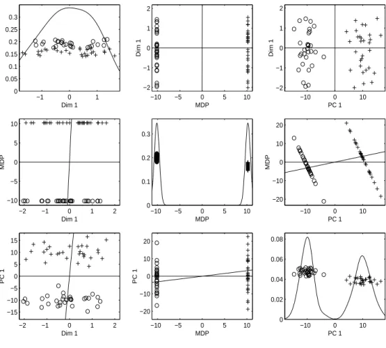
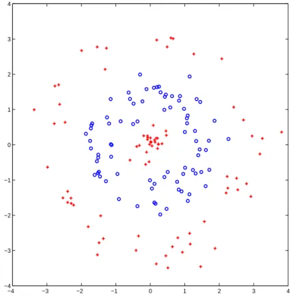
As it is difficult to visualize HDLSS data, projecting the data vectors to low dimensional spaces, especially to a one dimensional vector or to a two dimensional plane can provide a limited, but useful way to look at the data set. Projections on three direction vectors of interest for a simulated HDLSS data set are shown in Figure 3.2. This toy data set has the dimension d = 4000 and sample size n = 60, generated from the multivariate Gaussian distribution with identity covariance matrix, with 30 observations from mean (0.1,· · ·,0.1)T,
shown with ‘+’ in the figure, and the other 30 from mean (−0.1,· · ·,−0.1)T, shown with ‘o’.
The three projection directions are the first coordinate direction (X1), i.e., (1,0,· · · ,0)T , the
MDP direction, and the first principal component direction (PC1). Note that PC1 is the direction with the largest variation in the whole data set. With the sample size increasing, the PC1 direction converges to √1
d(1,· · · ,1)
T, which is the optimal direction to discriminate the
two classes.
Projections onto each of these three directions are shown in the three diagonal panels. In each diagonal panel, a “jitter plot” (Tukey and Tukey, 1990) is displayed for each class: The projected data are shown with random vertical coordinates for visual separation of the data. Also kernel density estimation curves are drawn to show how the projected values are distributed. The off-diagonal panels show the projections onto the planes spanned by each pair of directions, which are shown with two solid lines in the panel. This type of display is called “draftsman’s view”.
Let us denote the panel in the r-th row and c-th column by “[r, c]”. For example, [1,2] is the (top, center) off-diagonal panel showing the projected data on the plane spanned by theX1
direction and the MDP direction. The first diagonal panel [1,1] of Figure 3.2 indicates that the difference between the two classes is not discernible in the X1 direction. The projected
data on the MDP direction shown in [2,2] are piled up completely at two points, one for each class. The panel [3,3] shows nice separation of the two classes by projecting the data onto the PC1 direction. The panels [1,2] and [2,1] show that the X1 direction is almost orthogonal to
−1 0 1 0 0.05 0.1 0.15 0.2 0.25 0.3 Dim 1
−10 −5 0 5 10
0 0.1 0.2 0.3
MDP
−10 0 10
0 0.02 0.04 0.06 0.08 PC 1
−10 −5 0 5 10
−2 −1 0 1 2 MDP Dim 1
−10 0 10
−2 −1 0 1 2 PC 1 Dim 1
−2 −1 0 1 2
−10 −5 0 5 10 Dim 1 MDP
−10 0 10
−20 −10 0 10 20 PC 1 MDP
−2 −1 0 1 2
−15 −10 −5 0 5 10 15 Dim 1 PC 1
−10 −5 0 5 10
−20 −10 0 10 20 MDP PC 1
plane of MDP and PC1 ([2,3] and [3,2]) show that these two directions are much closer to each other, which means the geometric representation of HDLSS data in Chapter 2 applies well for this toy data set.
3.3 Mathematics of the MDP Direction
In this section we express the MDP direction vector in a closed form and show that it is uniquely determined within the subspace generated by the data. Also, we show that it is equivalent to the FLD direction vector when the dimensiondis less than or equal to the sample size minus two, i.e., when d6n−2.
Let X = (x1,· · ·,xn1) be the matrix of the training data from Class +1, where the xi’s
are random column vectors from a continuous probability distribution in Rd, and defineY =
(y1,· · ·,yn2) for Class−1 in a similar way. Letn=n1+n2. Define thed×ncombined data
matrix Zas [X,Y], the horizontal concatenation of the matrices X and Y, using Matlab-like notation. Denote the global sample mean vector of the combined data by ¯z. Then the sample covariance matrix ofZis
e
Σ≡ 1
n−1{(Z−Z)(Z¯ −Z)¯
T},
(3.14)
where ¯Z= ¯z1T
n. We will call the matrix Σe the global sample covariance matrix.
The MDP direction vector is defined as
vMDP≡
˜
Σ−(¯x−y)¯
kΣ˜−(¯x−y)k¯ , (3.15)
whereA− is the Moore-Penrose generalized inverse of a matrixA. The MDP direction vector exists if the data vectors are linearly independent, which is satisfied with probability one when the underlying distribution of the data is continuous inRd.
3.3.1 Characterization of the MDP Direction Vector in the Data Space
subspace inRd and this subspace is expressed as
SZ={Zw:w∈ Rn}. (3.16)
In other words, SZ is the set of all linear combinations of the data vectors. If we let HeZ be
the hyperplane generated by Z, then we can write
e
HZ={Zw:wT1
n= 1,w∈ Rn}. (3.17)
Note thatHeZ is a set of linear combinations of data points of which the sum of the coefficients
is one. The parallel subspace can be found by shifting the hyperplane so that it goes through the origin. A natural shift is via the point inHeZthat is closest to the origin which is calculated
in the following lemma.
Lemma 3.3.1. Let vZ be the point in HeZ that is nearest to the origin. Then,
vZ= Z(Z
TZ)−11 n
1T
n(ZTZ)−11n
.
Proof. Since vZ is on the hyperplane HeZ, it can be expressed in the form vZ = Zw, where
wT1
n= 1,w∈ Rn by (3.17). The squared distance from the origin tovZ is wTZTZw and we
need to find w that minimizes this distance. The Lagrangian (Cristianini and Shawe-Taylor, 2000, Chapter 5) of this minimization problem is
L(w) = 1 2w
TZTZw−α(1T
nw−1),
whereα>0 is the Lagrangian multiplier. From ∂L(w)/∂w= 0,
FromwT1
n= 1,
α = 1
1T
n(ZTZ)−11n
.
Thus,
vZ=
Z(ZTZ)−11 n
1T
n(ZTZ)−11n
.
Now let us shift the hyperplane HeZ so that it contains the origin and call the new shifted
hyperplaneHZ. Because HZ =HeZ−vZ,
HZ =
Zw:w∗=w− (Z
TZ)−11 n
1T
n(ZTZ)−11n
,wT
1n= 1,w∈ Rn
= {Zw∗ :w∗T1
n= 0,w∗∈ Rn}. (3.18)
Note that HZ is a subspace of Rd with dimension n−1 and we can decompose S
Z into an
orthogonal sum of HZ and {vZ}, i.e., SZ = HZ⊕ {vZ}. In the same fashion we can define subspaces parallel to the hyperplanes of X andY, call them HX and HY, respectively. They
have the following expressions:
HX =
Xw∗1 :w1∗=w1−
(XTX)−11 n1
1T
n1(X
TX)−11 n1
,wT
11n1 = 1,w1 ∈ R
n1
= {Xw∗1 :w∗T
1 1n1 = 0,w
∗
1∈ Rn1}, (3.19)
HY =
Yw∗2 :w∗2 =w2−
(YTY)−11 n2
1T
n2(Y
TY)−11
n2
,wT
21n2 = 1,w2 ∈ R
n2
= {Yw∗2:w∗T
2 1n2 = 0,w
∗
2 ∈ Rn2}. (3.20)