The Impact of Health Insurance on Medical Care,
Lifestyle Behaviors and Health of Non-Elderly Diabetics
by Betty T. Tao
A dissertation submitted to the faculty of the University of North Carolina at Chapel Hill in partial fulfillment of the requirements for the degree of Doctor of Philosophy in the Department of Economics.
Chapel Hill 2007
Approved by:
c
2007
Betty T. Tao
ABSTRACT
BETTY T. TAO: The Impact of Health Insurance on Medical Care, Lifestyle Behaviors and Health of Non-Elderly Diabetics
(Under the direction of Donna B. Gilleskie)
This dissertation examines the impact of health insurance coverage on diabetics’ decisions to monitor, treat and manage their condition and gauges the effect of these decisions on their health. Diabetics can experience serious or fatal complications with-out regular monitoring (of blood glucose and other indicators of disease severity) and, in some cases, prescription medication. These activities can present a significant fi-nancial burden that could be substantially attenuated by health insurance. Through cross-price effects, insurance may also influence important lifestyle choices such as ex-ercise and diet. However, insurance status is likely to be determined simultaneously with these behaviors in shaping health. Using a sample of non-elderly diabetics from the Medical Expenditure Panel Survey, I jointly estimate demand equations for health insurance, medical treatment, lifestyle decisions and health, controlling for their com-mon unobserved determinants. I find that insurance with drug coverage leads to better adherence to diabetic care guidelines. Furthermore, the presence of insurance lowers the probability of eye and kidney problems. I estimate that individuals value the for-mer at over $40,000. There is, however, some evidence of ex ante moral hazard: those covered by insurance with a drug plan show slightly lower probabilities of exercising regularly. I also use alternate model specifications to test the robustness of results.
ACKNOWLEDGMENTS
I am extremely grateful to my advisor, Donna Gilleskie, who not only guided my research for the past five years, but provided inspiration by showing me that some-one can be successful in such a competitive field while maintaining a balanced life. I am indebted to Tom Mroz, whose knowledge and encouragement always gave me the motivation to continue, even when I thought things were bleak. I must thank John Akin as I always leave his office with a new, improved perspective on research and life. I cannot thank Helen Tauchen enough- her dedication to students and ability to ex-plain complex ideas in an understandable manner epitomizes my image of a university professor. I would like to also thank Edward Norton and Peter Lance, whose input has been invaluable to me.
My family deserves special acknowledgement. They have always been so proud of anything I accomplished, no matter what it was. Thank you Mom, Dad, Juliane, Brian and Tyler. I would also like to give a special thanks to Hamilton Fout, Emil Rusev, the Rowdies and all my friends who have made the last five years worth it.
TABLE OF CONTENTS
LIST OF TABLES
x
LIST OF FIGURES
xiv
1 Introduction 1
1.1 Motivation . . . 1
1.2 My Contribution . . . 4
1.3 Overview of Chapters . . . 4
2 Background 5
2.1 Health Insurance . . . 5
2.2 Effects of Health Insurance on Health . . . 6
2.3 Diabetes . . . 9
3 Theoretical Model 11
3.2 Individual Choices . . . 12
3.3 Utility . . . 12
3.4 Constraints . . . 13
3.5 Health Production . . . 14
3.6 Bellman Equation . . . 14
4 Data 17 4.1 Medical Expenditure Panel Survey . . . 17
4.1.1 Health Insurance . . . 18
4.1.2 Health Inputs . . . 20
4.2 Health Outcomes . . . 21
4.3 Variation in Health Outcomes and Behaviors by Insur-ance Type . . . 22
5 Empirical Framework 28 5.1 Equation Specification . . . 28
5.2 Estimation Strategy . . . 31
5.2.1 Identification . . . 33
5.2.2 MEPS Primary Sample Units . . . 34
6 Results and Simulations 38
6.1 Goodness of Fit . . . 38
6.2 Empirical Findings . . . 39
6.2.1 Insurance Effects . . . 39
6.2.2 Health Production . . . 41
6.3 Health Insurance Simulation . . . 43
7 Other Specifications 56 7.1 Alternative Health Insurance Definition . . . 56
7.2 Omitting Those On Insulin . . . 56
7.3 Exclusion of Medicaid and Medicare Enrollees . . . 57
7.4 Additional Measures of Health . . . 58
7.4.1 Including Heart Attacks and Strokes . . . 58
7.4.2 Including Hospital Nights . . . 60
7.5 Effects of Diagnostic Care on Lifestyle Practices . . . 60
7.6 Medical Care Utilization . . . 61
7.7 Education . . . 61
8.1 Discussion . . . 73
8.2 Future Work . . . 74
A Estimation Results 76
LIST OF TABLES
4.1 Sample Determination . . . 23
4.2 Summary Statistics: Exogenous Variables . . . 24
4.3 Summary Statistics: Insurance, Health Inputs and Health Outcomes . . . 25
4.4 Percentage of Each Insurance Type in Time 1 and 2 . . . 26
4.5 Percentage of Each Insurance Type in Time 1 and 2 . . . 26
4.6 Percentage with Eye Problems in Time 1 and 2 . . . 26
4.7 Percentage with Kidney Problems in Time 1 and 2 . . . 26
4.8 Means of Key Variables By Insurance Type . . . 27
6.1 Comparison of Model Mean Predicted Values and Actual Mean Values . . . 47
6.2 Distribution of Unobserved Heterogeneity from Estimation . . . 47
6.3 Marginal Effect of Insurance with Drug Coverage on Di-agnostic, Medical Care and Lifestyle Behaviors . . . 48
6.5 Marginal Effects of Diagnostic Care and Input Behaviors
on the Probability of Eye and Kidney Problems . . . 50
6.6 Unobserved Heterogeneity Coefficients from the Joint
Es-timation . . . 51
6.7 Insurance Simulation on Diagnostic, Medical and Lifestyle
Behaviors: Level and Percentage Point Changes . . . 52
6.8 Insurance Simulation on Diet, Exercise and Medications
Trade-off: Level Percentages and Percentage Point Changes . . . 53
6.9 Insurance Simulation on Health Outcomes: Level
Per-centages and Percentage Point Changes . . . 54
7.1 Insurance Simulation: Level and Percentage Point Changes
with Alternative Insurance Definition . . . 63
7.2 Simulation: Level Percentages With Only Those Not on Insulin . . . . 64
7.3 Insurance Simulation: Level Percentages Without
Med-icaid and Medicare Enrollees . . . 65
7.4 Heart Attack: Selected Logit Results . . . 66
7.5 Stroke: Selected Logit Results . . . 67
7.6 Insurance Simulation: Level Percentages Including
Addi-tional Health Outcomes . . . 68
7.7 Hospital Nights: Selected Logit Results . . . 69
7.8 Insurance Simulation: Level Percentages With
Alterna-tive Insurance Pathway . . . 70
7.9 Insurance Simulation: Level Percentages Including Addi-tional Health Inputs . . . 71
7.10 Diagnositc Care Interacted With Education: Health Pro-duction Logit Results . . . 72
A.1 Estimation Results for Initial Health . . . 76
A.2 Estimation Results for Health . . . 77
A.3 Estimation Results for Eye Problem . . . 79
A.4 Estimation Results for Kidney Problem . . . 81
A.5 Estimation Results for Insurance . . . 83
A.6 Estimation Results for HBA1c Blood Glucose Test . . . 84
A.7 Estimation Results for Feet Checked . . . 85
A.8 Estimation Results for Cholesterol Checked . . . 86
A.9 Estimation Results for Eyes Checked . . . 87
A.10 Estimation Results for BP Checked . . . 88
A.12 Estimation Results for Input Behaviors: Exercise Only
vs. None . . . 90
A.13 Estimation Results for Input Behaviors: Oral
Medica-tions Only vs. None . . . 91
A.14 Estimation Results for Input Behaviors: Diet and
Ex-ericse Only vs. None . . . 92
A.15 Estimation Results for Input Behaviors: Diet and Oral
Medications Only vs. None . . . 93
A.16 Estimation Results for Input Behaviors: Exericise and
Oral Medications Only vs. None . . . 94
A.17 Estimation Results for Input Behaviors: Diet, Exericise
and Oral Medications vs. None . . . 95
LIST OF FIGURES
3.1 Timing of key variables. . . 13
5.1 Variation in Insurance by PSU . . . 36
5.2 Variation in Insurance Without Drug Coverage by PSU . . . 36
5.3 Variation in Union Penetration by PSU . . . 37
6.1 Simulation: Percentage with Eye Problems Over 40 Years . . . 55
Chapter 1
Introduction
1.1
Motivation
Over 20 million people in the United States suffer from diabetes mellitus and the number is projected to increase rapidly, as an estimated 41 million Americans are pre-diabetic.1 Diabetics produce either low levels of insulin or insulin that cannot regulate
blood sugars. The resulting higher levels of blood glucose can compromise a wide range of body tissues and organs. For example, diabetes is the leading cause of adult blindness, kidney failure and amputations.
Type 2 diabetes, which accounts for over 90 percent of diabetes cases, requires ongoing medical attention both to limit complications and to manage them when they do occur. Diabetes care guidelines mandate regular measurement of blood glucose levels, foot and eye examinations and regular checkups, all of which can become quite costly. Furthermore, over 60 percent of diabetics require oral medications to lower blood sugar levels and many need additional medicines to help control cholesterol and
1According to the CDC’s “National Diabetes Fact Sheet,” 14.6 million people have been diagnosed
blood pressure.2 As a result, they experience much higher health expenditures than the
general population. For instance, in 2002 total per capita medical care expenditures were $13,243 for diabetics and $2,560 for non-diabetics (American Diabetes Association 2002). Successful management also requires lifestyle changes, such as exercise and improved nutrition, that may delay or even completely prevent diabetes complications.3 However, these can be costly as well.
Adherence to these guidelines has important implications for the course of the dis-ease. Detection and treatment of diabetic eye disease can reduce severe vision loss by an estimated 50 to 60 percent, while controlling blood pressure limits the decline in kidney function by 30 to 70 percent. Comprehensive foot care programs can reduce amputation rates by 45 to 85 percent. Indeed, these interventions could ultimately be cost saving. Diabetes management programs such as the Asheville Project and the more recent Diabetes Ten City Challenge enlist employers to actively encourage their workers to care for their diabetes by providing regular exposure to trained pharmacists and waiving co-payments on medication and monitoring supplies. Although total med-ical costs increased initially, they fell in subsequent years and job absenteeism was cut by 50 percent.
Health insurance lowers the out-of-pocket price of medical care and in the process, possibly influences lifestyle choices via cross-price effects. For example, some may use more medical care when insured, but devote fewer resources to exercising and preparing healthy foods, dampening any positive effects of insurance on health. This
2This figure is compiled by the Centers for Disease Control and Prevention (CDC) using data from
the National Health Interview Survey in 2005. Those with type 1 and more severe cases of type 2 diabetes require insulin.
3Even for people already diagnosed with diabetes type 2, weight loss may make insulin more effective
paper examines the role of insurance in determining the medical care consumption, health behaviors and health of non-elderly diabetic adults. I focus on the non-elderly since over three-fourths of diabetics age 18 through 79 are diagnosed before age 60 and half are diagnosed between 40 and 59 (Centers for Disease Control and Prevention 2004). Their decisions will have a substantial impact on the trajectory of the disease as they age. Using the diabetes care supplement to the Medical Expenditure Panel Survey, I investigate the impact of health insurance and prescription drug coverage on diabetics’ decision to monitor the disease, to use various treatments recommended under the diabetic care guidelines and, indirectly, to modify their lifestyle. Since policymakers ultimately care about health, I also estimate a health production function that captures the relative productivity of different types of health behaviors in determining health. I examine a measure of overall health as well as more specific diabetes-related outcomes, such as the presence of eye and kidney problems.
I compare several methods to account for the endogeneity of insurance, health inputs and health, ranging from a two-stage least squares instrumental variables approach to a joint estimation of the demand for health insurance, medical care, health behaviors and health. Through simulations, I assess the effect of insurance on the frequency of checkups and examinations, the use of medications, lifestyle choices and, through these inputs, on health. Additionally, I include various different specifications to test the robustness of the model.
Joint estimation of insurance, medical care demand, lifestyle behavior and health production equations that account for time invariant unobserved heterogeneity reveals that the presence of insurance increases the likelihood of adhering to diabetes care guidelines and that these behaviors do indeed improve health. Simulations show that insurance with drug coverage leads to a three percentage point decrease in the probabil-ity of diabetic eye problems and a two percentage point decrease in the probabilprobabil-ity of a
kidney problem. Using figures from the literature on the disutility of blindness and the value of life, this reduction in the probability of blindness is valued at approximately $40,000. However, I find some evidence of ex ante moral hazard in that insurance with drug coverage is associated with a drop in the probability of exercising regularly.
1.2
My Contribution
This paper contributes to the literature by determining the impact of health insur-ance on the behavior of diabetics and health outcomes through an estimation procedure that accounts for the joint nature of the insurance, medical care and lifestyle behavior decisions. I use a sample of diabetics from a nationally representative survey, allowing for more objective measures of health outcomes. Furthermore, I examine cross-price effects of insurance coverage on medical care demanded and lifestyle behaviors that are believed to play a major role in the health of diabetics.
1.3
Overview of Chapters
Chapter 2
Background
2.1
Health Insurance
not vary much by insurance coverage (Manning et al., 1987). Other studies have found a significant impact of health insurance on medical care demand. Using Australian data from 1977-1978 Cameron et al. (1988) find evidence that more generous insurance coverage increases the use of health services after controlling for selection into different plans.
More recently, focus has turned to the effects of insurance policies with differen-tial cost-sharing by service type. In particular, several studies examine the cross-price effects of increased prescription drug cost-sharing. A Canadian study finds that an in-crease in drug copayments among the elderly is associated with a reduction in utilization that leads to greater use of hospital emergency rooms and increased hospitalizations and a rise in overall health care costs (Tamblyn et al., 2001). Yang, Gilleskie and Norton (2004) estimate a dynamic model of medical care demand and health using data from the Medicare Current Beneficiary Survey to examine cross price effects be-tween prescription drugs, physician services, hospital care and the subsequent impact on health from the presence of prescription drug coverage. They show that universal prescription drug coverage would increase drug expenditures by 20 to 35 percent over five years while inpatient and physician service use would increase only slightly. Most of this increase is attributed to reduced mortality.
2.2
Effects of Health Insurance on Health
for myopia correction and dental problems. Although the study found no significant benefits for the average person, the authors admit that the health outcomes examined were relatively common chronic conditions where a diagnostic test was rather inexpen-sive.1 Most other studies that examine the health effects of insurance policy changes focus on supply-side cost sharing mechanisms, such as Medicare’s prospective payment of hospital services, and the results have not been conclusive (Cutler and Zeckhauser, 2000).
Furthermore, moral hazard in health insurance adds complications by reducing in-centives for prevention.2 Ehrlich and Becker (1972) use an expected utility model in
which individuals can respond to any type of uncertainty by purchasing market in-surance that provides income should a bad state occur, by engaging in self-protection activities that reduce the probability of a bad state and by engaging in self-insurance activities that reduce the loss from a bad state. This model can be easily applied to health. Self-protection that reduces the probability of a bad state refers to self-preventative measures such as brushing teeth and losing weight whereas self-insurance involves diagnostic medical care such as mammograms and physicals. Market insur-ance, in the extreme case, refers to health insurance that covers catastrophic health outcomes such as cancer. If market insurance premiums are actuarially fair and ac-count for self-protection activities, individuals will have the correct incentives, since spending on self-protection lowers the cost of market insurance and individuals will purchase the optimal amount of both. However, the informational asymmetry that oc-curs from insurers’ inability to observe self-protection activities leads to underspending on self-protection and overspending on market insurance. With this type of
external-1Manning et al. thus argue that money spent on better screening for the poor would be more cost
effective than full insurance.
2Moral hazard here refers to ex ante moral hazard, since the concern is the effect of insurance
on actions the individual takes before knowing his health state. Ex post moral hazard refers to the behavior of individuals once the health state is known, such as purchasing too much curative care.
ity, an insured individual ignores the effect of his own self-protection spending on the premiums paid by others in the insurance pool. Empirical evidence points towards a small moral hazard effect of purchasing market insurance, but is not conclusive (Kenkel, 2000). Additionally, Ehrlich and Becker argue that since the price of self-insurance is not related to the probability of the negative event, it is likely to create a moral hazard as well. They find market insurance and self-insurance to be substitutes, but in practice health insurance coverage for each of them are commonly under one contract with the same insurer, making it more difficult for individuals to choose the optimal amount of both.
It may not always be the case that individuals substitute medical care for self-protection because it is possible that market insurance and self-self-protection may be complements. More self-protection can increase the marginal product of market insur-ance in that increased self-protection can lower the probability of a bad state, which may be rewarded by market insurance. Self-protection is encouraged if the price of market insurance is negatively related to the amount spent on protection. This occurs in the automobile industry where time spent accident-free commonly lowers premiums, but it is not common in health insurance markets (although the presence of a pre-existing conditions makes it more difficult to switch insurers and this can be viewed as an increase in price.)
2.3
Diabetes
Another difficulty in estimating effects of health insurance on health outcomes is choosing the proper measure of health. If health is defined as the mortality rate or life expectancy, one might be led to conclude that the marginal contribution of medical care use has been zero in the past few decades in developed nations. Other measures such as Quality Adjusted Life Years (QALYs) have been used, but these also have limitations since translating additional years of life into QALYs can be difficult with chronic conditions that lower the quality of life, but are not fatal.
Using diabetics for analysis mitigates the problems with finding an adequate health definition, since more “objective” measures of health can be used, such as the pres-ence of diabetic-related eye and kidney problems. Furthermore, the lifestyle choices of type 2 diabetics factor heavily in the likelihood of contracting the disease as well as in controlling the severity of the symptoms. Self-prevention in diabetics via better lifestyle habits is relatively low cost and highly beneficial. Although the results will not translate to the average individual in average health, diabetes is a rapidly growing problem affecting more and more of the world population.3 According to the
Amer-ican Diabetes Association, the total cost of diabetes, including direct costs in terms of medical expenditures and indirect costs in terms of lost work days and permanent disability, was $132 billion in 2002. The true burden of diabetes is likely to be even higher as an estimated 6.2 million people went undiagnosed with diabetes in 2005.
Delays or noncompliance in recommended health care behavior may result in a substitution toward other types of medical care that may be costlier and less effective. A recent study of a group of diabetics finds that 17-33 percent receive no diabetes medication whatsoever. Those who do not use any drug medication have 18 percent
3For example, with more sedentary lifestyles, China is facing an explosion in the prevalence of
obesity-related diabetes. In a survey from 19 provinces of China, the prevalence has tripled from 1970 to 1990.
more physician visits and 15 percent more days in the hospital (Pharmetrics, 2004). All individuals in this study are covered by some type of insurance, indicating that these results represent a lower bound on the noncompliance of diabetics. In fact, 20 percent of diabetics 18 through 64 were completely uninsured in 2002.4 Furthermore, Niefeld et al. (2003) find that seven percent of all hospitalizations among type 2 diabetics can be avoided by improved outpatient care of comorbidities. This is likely an upper boundary on preventable hospitalizations, as they examine elderly diabetics, where comorbidities are much more common.
Multiple studies find that medical care and self-care practices are sub-optimal and that the majority of type 2 diabetics are overweight and do not follow dietary guidelines (Hiss, 1996; Harris, 1996; Nelson et al., 2002). Using claims data from nine large firms, Dor and Encinosa (2004) estimate that an increase in the coinsurance rate from 20 percent to 75 percent results in an increase in the share of diabetics who never comply with prescriptions by 9.9 percent. It reduces the share of fully compliant diabetics by 24.6 percent. They find that this decrease in drug expenditures amounts to $125 million nationally, but leads to health complications that would cost an additional $360 million in treatment. This number comes from a rough estimate of the higher expenditures of diabetics with poor glycemic controls.
I use a sample of diabetics from a nationally representative survey to examine the cross-price effects of insurance coverage on medical care demanded and lifestyle behaviors that are believed to play a major role in the health of diabetics. The next section describes the theoretical model, which is the basis for the empirical results.
Chapter 3
Theoretical Model
3.1
Motivation
The seminal work by Grossman (1972), describing a human capital approach to health, provides a framework for examining individual-level health care demand and health production. In Grossman’s model, health is a depreciating stock in which indi-viduals must invest over time. Indiindi-viduals do not receive utility from medical services directly, but only through their positive effects on health.
behaviors subject to a per period budget constraint and time constraint.
3.2
Individual Choices
At the beginning of each period t, the individuali observes his health entering the period and selects among health insurance alternativesj, denoted byIitj, where
j =
0 uninsured
1 health insurance without drug coverage 2 health insurance with drug coverage
(3.1)
and P2
j=0I j it = 1.
The individual also chooses the level of several health behaviors. These include diagnostic medical care Dit =d, medical care Mit =m and lifestyle behaviors Lit =l,
conditional on his choice of insurance. Figure 3.1 depicts the timing of choices. For simplicity, I drop the isubscript from all variables from here on.
3.3
Utility
The individual receives utility from consumptionCt, healthHtand leisureSt. Utility
is described as
Ut=U(Ct, Ht, St) (3.2)
where ∂Ut ∂Ct >0,
∂Ut
∂Ht >0 and ∂Ut
Figure 3.1: Timing of key variables.
Note: An individual enters the period with health status Htand chooses his insurance plan Itbefore
observing health shock,t. He then chooses health inputs,Dt,MtandLt. Based on these choices
andt, health is updated toHt+1 through the health production function.
3.4
Constraints
The individual allocates income between a composite consumption good and medical services. The budget constraint is
Yt=Ct+P rjtI j t +a
j
tDt+bjtMt+ctLt (3.3)
whereYtis income of the individual at timet. Ctis a composite consumption good with
the price normalized to 1, P rtj is the per period premium associated with plan j where
P r0
t = 0 and a j t and b
j
t represent the out-of-pocket responsibility of the consumer with
insurance planj where a0 = 1 and b0 = 1. IfM
t is viewed as prescription medications,
then b1 = 1. c
t represents the monetary cost associated with lifestyle behaviors. Let
Pt= (P rjt, a j t, b
j
t, ct) be a vector of exogenous monetary price variables.
The individual also faces a time constraint. Since I do not model the decision on the amount of hours worked, I abstract from the work decision and ¯T represents the amount of time left over in a period after work. The remaining hours can be split on leisure and on lifestyle behaviors: ¯Tt=St+Lt.
3.5
Health Production
Health in the next period is determined by health and health inputs in the current period. That is,
P(Ht+1=h) = fh(Ht, Dt, Mt, Lt, Xt, t) h= 1, ..., H (3.4)
where t represents a health shock that affects the probability of entering each health
state. ∂H∂f
t > 0, ∂f
∂Dt > 0, ∂f
∂Mt > 0, ∂f
∂Lt > 0 and all second derivatives are negative
(diminishing marginal returns). Xt is a set of exogenous socio-demographic variables
such as education, marital status, race and age.
3.6
Bellman Equation
Individuals in this model begin at time t = 1 and continue until t = T+1 at which time they die. The objective of the individual is to choose a level of diagnostic care, medical care, lifestyle activity and insurance plan so as to maximize his lifetime utility. He must choose his insurance plan prior to the realization of his health shock, but chooses the level of health inputs after the realization. Health evolves through a production function that depends on the health shock and level of health inputs. State variables include Ht, Xt, Pt and t. Written as a Bellman equation and substituting
Dt =d, Mt=m, Lt=l at time att conditional on Itj = 1 and with t known is
Vjt(Ht, Xt, Pt|Itj, t) = Ut(Yt−P rtjI j t −a
j
tDt−bjtMt−ctLt, Ht,T¯t−Lt)+
+β
H X
h=1
P(Ht+1 =h|Ht, Dt, Mt, Lt, Xt, t)Wt+1(Ht+1, Xt+1, Pt+1)
.
(3.5)
At the beginning of time t, t is not known. The maximal expected value of lifetime
utility conditional on a particular insurance alternative is
Vjt(Ht, Xt, Pt|I j t) = Et
max
Dt,Mt,Lt
Vjt(Ht, Xt, Pt, t|I j t)
(3.6)
The maximal expected lifetime utility unconditional on a particular insurance alterna-tive (the last component of 3.5, but in time t) is
Wt(Ht, Xt, Pt) = max Itj
V0t(Ht, Xt, Pt),V1t(Ht, Xt, Pt),Vt2(Ht, Xt, Pt)
where Itj ∈ {0,1},
2
X
j=0
Itj = 1.
(3.7)
At t = T, the individual knows he will die the next period and therefore will not buy insurance (IT0 = 1), will not use diagnostic care and medical care and will not spend any time on lifestyle activities. T is thus a high age such as 125 years. The value of lifetime utility at time T is thus
VT =UT(YT, HT =h,T¯T). (3.8)
Solving this optimization problem requires imposing functional forms for health production and utility and leads to demand equations for Dt, Mt, Lt and insurance
Chapter 4
Data
4.1
Medical Expenditure Panel Survey
The Medical Expenditure Panel Survey (MEPS), which first began in 1996, collects data on medical care utilization, costs, and the sources of payment of a nationally rep-resentative sample of Americans. The data contain health status measures, utilization and expenditure by medical service, income and demographic measures. The MEPS household survey follows individuals over two years with five rounds of interviews. In each round, sample members are asked to recall medical conditions and expenditure events since the last interview, with supplemental information collected from medical providers identified by household respondents. Data collection rounds are launched with a new sample each year, providing overlapping panels of survey data. Currently, Panels 1 to 7, which cover 1996 to 2003 and include over half a million individual interviews, are available.
caused any kidney or eye problems. Information is gathered twice from each individual over the two years. MEPS first began administering the DCS in 2000, with Panel 4, and continued through Panel 7. Using information from the DCS combined with the MEPS household survey allows for detailed analyses of the health care decisions of di-abetics between 1999 and 2003. I am aware of only one other nationally representative data set with information on diabetics- the National Health Interview Survey (NHIS), administered by the Centers for Disease Control and Prevention. The NHIS interviews individuals only once, making analysis on the effects of insurance on health inputs and health outcomes difficult due to the timing of decisions.
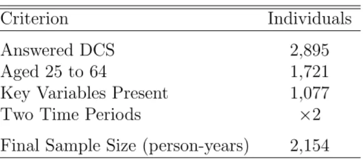
Data from the DCS are collected once a year over two years providing two observa-tions for each individual, but other variables are collected five times over the two years, allowing for the definition of an initial health condition. The total number of diabetics that answered all or some of the DCS is 2,895. After restricting the sample by age and the presence of key variables, the final sample of 2,154 person-years is comprised of 1,077 individuals observed twice and covering years 1999 to 2003. Table 4.1 displays the sample selection details.
The summary statistics of exogenous variables are in Table 4.2. Average age is 51 and the sample is evenly distributed with males and females. Fifty percent of the sample report finishing High School as their highest degree. The latter portion of the table report the means of exclusion restrictions.
4.1.1
Health Insurance
drug coverage. Those on Medicaid are considered insured with drug coverage. Table 4.3 lists the sample means for the key variables. Five and a half percent report being insured with no drug coverage. Twenty-four percent of the sample report purchasing no insurance plan whatsoever.1
Table 4.4 shows how insurance changes over the two time periods. The majority (82%) retain health insurance with drug coverage over the two time periods. Thirteen percent remain uninsured both years and the remaining six percent switch coverage over the two years. Health insurance here is defined using a variable in MEPS that turns on if the individual was uninsured the entire year.
MEPS does not collect information on whether the individual did or did not have prescription drug coverage the entire year. Instead, the information is collected for each round of the 5 rounds MEPS interviews sample members. Thus, as an alterna-tive health insurance variable, I use information from the rounds in each year. If an individual had insurance in the first round of one year, but not the next two, he was considered uninsured. Table 4.5 shows the percent of individuals who switch insur-ance coverage between there two years including insurinsur-ance without drug coverage as a separate category.
The diabetics individuals in my model choose their insurance type. However, in-dividuals in my sample are all diabetics and it is possible the uninsured were unable to obtain insurance. Under the Health Insurance Portability and Accountability Act of 1996, it was made illegal to be refused coverage into a group plan based on an pre-existing condition if one had “credible” coverage for the previous 12 months. However, there is no protection when moving from one individual (privately purchased) plan to another. MEPS gathers information on whether an individual was ever denied insur-ance. Very few people (18) in my sample reported ever being denied insurance due
1Based on Census data, 19 percent of individuals age 18-64 were uninsured in 2004.
to their diabetes and of these only 5 reported to actually be uninsured. Furthermore, these individuals appear to be evenly distributed across health outcomes.
Employer-provided insurance remains the most common way to obtain insurance in this country. It is therefore arguable that individuals choose their job and health insurance is ancillary. However, there is evidence that individuals who are offered health insurance through the employer may not take it. I find that 35% of those who are insured are not employed and 45% of uninsureds are not employed. Of the 35% who are insured but are not employed, about 40% are not married and thus would not be receiving health insurance through a spouse. I found very few people in my sample to be self-employed.
4.1.2
Health Inputs
Diagnostic outcomes include variables on whether the individual obtained a blood glucose HbA1c test at least twice in the last year, a foot examination in the last year, an eye examination (with pupils dilated) in the last year, a blood pressure checkup in the last three months and a cholesterol test in the last year. As shown in Table 4.3, 76 percent of the sample checked their blood glucose using a Hemoglobin A1c test at least twice in the past year. The American Diabetes Association recommends a frequency of two to four tests a year. According to a study administered by the Centers for Disease Control and Prevention in 2004, 72 percent of adults with diabetes had their A1c tested at least twice.2 The figures for the other diagnostics are similar as well.
Input behaviors in Table 4.3 include whether the individual currently treats diabetes with diet modifications and/or whether he exercises at least three times a week. While 80 percent of the sample say they have modified their diet to treat their diabetes, only 40 percent exercise at least three times a week. Three quarters of the sample
2The source is the Centers for Disease Control and Prevention’s National Diabetes Surveillance
report the use of oral medications for diabetes treatment. I create eight mutually exclusive combinations of the three input behaviors in order to examine relative trade-offs between each category. Fewer than 10 percent of the sample engage in only one activity and five percent report engaging in none of the behaviors. Almost 40 percent use oral medications in conjunction with diet modifications, but only four percent supplement oral medications with regular exercise. Twenty-seven percent of the sample exercise regularly, modify their diet and use oral medications.
4.2
Health Outcomes
Health is measured by general health status and the presence of eye or kidney problems. Diabetic-retinopathy is the most common diabetes related eye condition and is found when diabetes has caused weaknesses and leakages in the blood vessels of the retina. In the worst case, new blood vessels form around the retina, which causes bleeding and swelling in the eye and results in partial or full blindness. Twenty-five percent report the presence of an eye problem. This figure is consistent with the CDC’s estimate that 20 percent of diabetics in the U.S. have moderate to serious eye problems. Diabetes is also the leading cause of kidney failure. Fourteen percent of the sample report the existence of kidney problems. This figure consistent with the 10 to 40 percent cited by the National Kidney Foundation. Forty percent of the sample report being in fair or poor health.
Table 4.6 presents the percentage of individuals who reports eye problems by year. Of the individuals with available observations in both years, 67 percent have an eye problem in both time periods and 16 percent do not have eye problems in both time periods. Eight percent report an eye problem in the second year and seven report not having an eye problem in the second after having one in the first year. Approximately
90 individuals do change eye status over the two years. Table 4.7 shows the same information for kidney problems. Kidney problems are less common than eye problems and 83 percent of individuals do not exhibit these problems in either year. Seven percent do have kidney problems in both years and the remaining ten percent change status over the two time periods.
4.3
Variation in Health Outcomes and Behaviors by
Insurance Type
Since my study examines the effects of insurance on behavior, it is interesting and important to descriptively see how health outcomes and behavior varies between those with and without insurance. The first part of Table 4.8 shows how health varies by insurance. A higher percentage of uninsureds report eye problems and being in worse health, though those with kidney problems appear to be equally distributed by insur-ance type. Diagnostic tests are more common among those who are insured. Surpris-ingly, the percentage of insureds who take oral medications to treat diabetes is not much higher than the uninsureds who use oral medications. A higher percentage of insureds modify their diet and exercise habits appear to be similar by insurance.
mean income for uninsureds of $35,000. The poverty line for a family of four in 2005 is $19,350. About 50 percent of the uninsured do have an income less than $25,000, which would in general quality them or their children for welfare benefits including Medicaid. However, they do not report being on Medicaid, but much of this might be due to low Medicaid take-ups rates (Aizer 2003).
Table 4.1: Sample Determination
Criterion Individuals
Answered DCS 2,895
Aged 25 to 64 1,721
Key Variables Present 1,077
Two Time Periods ×2
Final Sample Size (person-years) 2,154 Note: Sample size is the number of individuals after selecting for each criterion. The final sample is 1077 individuals over two time periods, or 2,154 person-years.
Table 4.2: Summary Statistics: Exogenous Variables
Variable Mean S.D.
Socio-demographic and Year Variables
Age 51.2 8.7
Family size 3.1 1.7
Income logged $45,474 37,870
Female 49.0
Black 17.0
Urban 74.6
Married 65.2
No degree 28.1
High school degree 50.3
College degree 11.0
MS or PhD 5.8
Other degree 4.7
Year 2000 26.4
Year 2001 27.4
Year 2002 32.1
Year 2003 14.1
Exclusion Restrictions Insurance
Market level: uninsured 28.1
Market level: insured without drug coverage 6.1 Market level: insured with drug coverage 65.8 Diagnostic Care and Input Behaviors
Distance to doctor: less than 15 minutes 45.4 Distance to doctor: less than 15 minutes 39.7 Distance to doctor: greater than 30 minutes 14.9 Transport to doctor: drives or is driven 94.4 Transport to doctor: drives or is driven 4.2
Transport to doctor: walks 1.4
Input Behaviors
Market level: Exercise 3 times per week 55.2 Initial Health
More likely to take risks† 1.1
No meds to get over illness† 0.7
Table 4.3: Summary Statistics: Insurance, Health Inputs and Health Outcomes
Variable (%) Mean
Insurance
Insurance, Drug 70.4
Insurance, no drug 5.5
No insurance 24.1
Diagnostic†
HBA1c test 2+ 75.7
Check feet 66.1
Check eyes 68.1
Check cholesterol 85.4
Check blood pressure 74.0
Input Behaviors
Modify diet 81.3
Exercise 3×per week 41.7
Use oral meds 74.3
Input Behaviors - Categories
None 5.3
Diet only 9.3
Exercise only 2.6
Oral meds only 7.2
Diet and exercise only 8.6
Diet and oral meds only 36.5
Exercise and oral meds only 3.7
Diet, exercise and oral meds 26.9
Health
Eye problem 25.5
Kidney problem 13.9
Health is excellent 22.3
Health is good 37.4
Health is poor/fair 40.1
†Diagnostic care variables are all yearly check-ups
except for blood pressure, where measurement is rec-ommended every three months.
Table 4.4: Percentage of Each Insurance Type in Time 1 and 2
Insurance in t= 2
Ins. Drug Uninsured
Insurance in t = 1 Ins. Drug 81.2 3.2
Uninsured 2.6 13.0
N = 1077 available observations in both years
Table 4.5: Percentage of Each Insurance Type in Time 1 and 2
Insurance in t= 2
Ins. Drug Ins. No Drug Uninsured
Insurance in t= 1
Ins. Drug 67.1 1.5 3.7
Ins. No Drug 1.0 4.5 0.0
Uninsured 3.7 0.5 18.0
Table 4.6: Percentage with Eye Problems in Time 1 and 2
Eye Problems in t= 2
No Yes
Eye Problems in t= 1 No 68.9 8.1 Yes 7.4 15.6
Table 4.7: Percentage with Kidney Problems in Time 1 and 2
Kidney Problems in t = 2
No Yes
Kidney Problems in t= 1 No 82.8 5.3
Table 4.8: Means of Key Variables By Insurance Type
Insurance with
Uninsured Drug Coverage
(N = 1844) (N = 343)
Health
Eye problem 25.1 27.6
Kidney problem 13.9 13.6
Health is excellent/very good 22.4 20.7
Health is good 36.8 36.7
Health is poor/fair 40.8 44.7
Diagnostic Behavior
HBA1c test 2+ 78.5 60.7
Check feet 67.8 57.0
Check eyes 70.8 53.7
Check cholesterol 87.6 73.3
Check blood pressure 76.0 63.4
Input Behaviors
Use oral meds 74.4 73.5
Modify diet 82.5 75.3
Exercise 3× per week 41.6 42.9
Socio-Demographic Variables
Female 49.6 54.5
Black 18.3 14.6
Urban 76.8 64.7
Married 65.4 63.0
No degree 24.7 44.0
High school degree 52.2 44.6
College degree 11.9 4.4
MS or PhD 5.7 4.7
Other degree 5.5 2.3
Age (years) 50.9 51.2
Family size 3.0 3.6
Income ($) 48,009 35,437
Chapter 5
Empirical Framework
5.1
Equation Specification
Solution to the theoretical model yields a set of demand equations for insurance, medical care, diagnostic care, lifestyle behaviors and a production function for health. A Taylor series expansion of the maximal lifetime value function, Vtj(Ht, Xt, Zt|Itj)
(Equation 3.6), suggests the following multinomial logit probability of choosing each insurance alternative. The dependent variable is the log odds that an individual chooses insurance alternative I0
t = 1 (uninsured) or It1 = 1 (insurance with no drug coverage)
relative toI2
t = 1 (insurance with drug coverage). Explanatory variables include health
entering period t, Ht, exogenous demographic variables Xt and a vector of relevant
exclusion restrictionsZtthat affect the individual’s decision to purchase insurance, but
are excluded from the medical care equations. Xt and ZtI are listed in Table 4.2. The
insurance equation is specified as
ln
P(Ijt = 1)
P(I2t = 0)
=δ0j+δj1Ht+δ2jXt+δ3jZ I t +ρ
j
whereµrepresents permanent unobserved individual heterogeneity with factor loading
ρj1 for insurance alternative j.1
The theoretical model implies a multiple outcome framework for estimating the di-agnostic, medical and lifestyle behavior equations. I use a multinomial logit to estimate the lifestyle and medical behaviors of exercising, modifying the diet and the using oral drugs for diabetes treatment. Including all combinations of the three behaviors results in eight mutually exclusive categories. Due to the number of diagnostic variables, I estimate the diagnostic equations each as binary logits. The log odds that an individ-ual chooses option b among the eight alternatives relative to engaging in none of the activities is a function of his insurance choice It, health Ht, exogenous factors Xt and
relevant exclusion restrictionsZtB (see Table 4.2). The eight alternative input behavior (Bt) multinomial logit is written as
ln
P(Bt =b)
P(Bt= 0)
=β0b+β1bIt+β2bHt+β3bXt+β4bZ B t +ρ
b
2µ, b = 0, ...,7. (5.2)
Similarly, the binary logit specification for each diagnostic equation is specified as
1The logit probability (simplified to a binary logit) is motivated as follows:
Utility(if insurance choice 0) = Vjt=0(Xt) =Xβ0∗+
∗
0
where Xt is a vector of state variables as described in Chapter 3 and the∗ indicates the value of
the parameter at the maximal expected lifetime utility level for a given insurance choice. Similarly,
Utility(if insurance choice 1) = Vjt=1(Xt) =Xβ1∗+
∗
1
The probability of an individual choosing insurance alternative 1 is
P(choose insurance choice 1) = P(Xβ1∗+∗1≥Xβ∗0+∗0).
Letβ∗=β∗
1−β0∗ and∗=∗0−∗1 The probability of choosing insurance alternative 1 is now
P(choose insurance choice 1) = P(Xβ∗≥∗) = logit(Xβ).
ln
P(Dt= 1)
P(Dt= 0)
=ψ0+ψ1It+ψ2Ht+ψ3Xt+ψ4ZDt +ρ3µ (5.3)
The health production function is modeled with a multinomial logit where the depen-dent variable is the log odds that an individual’s health next period is h where h = 0 (fair/poor health) or h = 1 (good health) or h = 2 (very good/excellent health). The explanatory variables include current healthHt, diagnosticDt, medicalMtand lifestyle
Lt care along with interactions with current health. The interactions allow more
flex-ibility in the relationship between current health and medical behaviors in explaining health next period. Health is written as
ln
P(Ht+1 =h)
P(Ht+1 = 2)
=αh0Ht+αh1Dt+αh2Lt+αh3Mt+αh4Ht×Dt
+αh5Ht×Lt+αh6Ht×Mt+α7hXt+ρh4µ, h= 0,1
(5.4)
where Xt includes the variables in the top portion of Appendix Table 4.2 excluding
income. Similarly, binary logit specifications are used for the probability of eye and kidney problems. They are written as
ln
P(Et= 1)
P(Et= 0)
=φ0Ht+φ1Dt+φ2Lt+φ3Mt+φ4Ht×Dt
+φ5Ht×Lt+φ6Ht×Mt+φ7Xt+ρ5µ
(5.5)
and
ln
P(Kt= 1)
P(Kt= 0)
=ϕ0Ht+ϕ1Dt+ϕ2Lt+ϕ3Mt+ϕ4Ht×Dt
+ϕ5Ht×Lt+ϕ6Ht×Mt+ϕ7Xt+ρ6µ.
Since lagged health is not observed for the first time period, I also estimate an initial health equation.
The error term for each equation is written as ρqµ+qt where q = 1,2, ..,6. It is
composed of a permanent, time-invariant unobserved individual factor µ, which does not vary across equations, but the effects of µ in each equation is measured by a factor loadingρe. qt are independent mean zero errors that are distributed logistically.
The equations must be estimated jointly since the error terms are correlated across equations. The following section describes the estimation method in detail.
5.2
Estimation Strategy
In order to obtain unbiased estimates of the parameters of the model, I must ac-count for the presence of unobserved heterogeneity that can lead to spurious correlation between dependent and explanatory variables. One way to do this is to treat the un-observed factor as a fixed individual effect. However, this would result in a loss of 1077 degrees of freedom and I observe only two time periods per person. Instead, I treat µ
as a random effect and integrate it out of the model. Instead of imposing parametric assumptions about the form of these terms, I use the discrete factor approach described by Heckman and Singer (1984), Mroz (1999) and Mroz and Guilkey (1992).
The discrete factor random effects framework assumes that µ consists of a distri-bution of heterogeneity that is approximated by discrete mass points with associated probability weights. These mass points and probability weights are estimated along with the parameters of the model. The conditional joint probability of observing the
data for each individual for all time periods is
Li(Θ|µ) = 2
Y
h=0
P(H1 =h|µ)H h i1 ×
T Y t=1 " 2 Y j=0
P(It=j|µ)I j it × 5 Y d=1
P(Ddt = 1|µ)Ddit
1−P(Ddt = 1|µ)
(1−Ddit)
×
8
Y
b=1
P(Bt=b|µ)B b it ×
2
Y
h=0
P(Ht+1 =h|µ)H h i,t+1
×P(Et+1 = 1|µ)Ei,t+1
1−P(Et+1 = 1|µ)
(1−Ei,t+1)
×P(Kt+1 = 1|µ)Ki,t+1
1−P(Kt+1 = 1|µ)
(1−Ki,t+1)
#
(5.7)
where Θ represents the parameters of the model (α’s, β’s, δ’s, ψ’s, φ’s, ϕ’s and ρ’s) and P(•) represents the logit or multinomial logit probabilities associated with the log odds equations from Section 5.1. The unconditional joint probability is obtained by summing over the number of time invariant mass points is written as
Li(Θ, θ) = M
X
m=1
θmLi(Θ|µm) (5.8)
wherem= 1, ..., M is the number of mass points andθmare the estimated weights
asso-ciated with each mass point. To estimate mass point locations and probability weights, I impose the appropriate normalizations. The likelihood function is then calculated by multiplying together the likelihoods for each individual:
L(Θ, θ) =
N
Y
i=1
Li(Θ, θ) (5.9)
order to ensure that the weights are between 0 and 1, the discrete factor model searches over a series of parameters, γm, that satisfy
θm =
exp(γm)
1 +PM−1
k=1 exp(γk)
(5.10)
wherem = 1, ..., M−1 mass points. The last weight is simply calculated by subtracting the estimated weights from 1. Mroz (1999) provides methods of choosing the optimal number of mass points.
5.2.1
Identification
The effects of insurance are identified theoretically by the price of insurance (premi-ums). Although these variables are not available, insurance characteristics of individu-als in the surrounding area can individu-also serve as variables that influence insurance purchase, but do not affect the demand for care. Because state or zip code level identifiers are not available in this public-use data set, I exploit information on all individuals in the primary sampling unit from which sample members were randomly selected for survey participation.2 I construct aggregate insurance characteristics that include whether or
not individuals have insurance and if so, whether or not they also have drug coverage at the primary sample unit level. MEPS draws survey participants from over 200 sampling units. For each individual, the aggregate insurance variable excludes that particular individual.
In order for the market level insurance variable to be a good instrument, it must be correlated with the endogenous variable, individual insurance. A regression of indi-vidual insurance type on market level insurance and other exogenous variables shows
2Rizzo and Zeckhauser (2005) use the share of generic scripts in each MEPS primary sampling
area as an instrument for an individual’s use of generic scripts in order to explain the price of brand-name scripts. They argue that this market-level measure proxies for laws in each sampling area that encourage generic substitution.
market level insurance and insurance without drug coverage to be jointly significant with a χ2 statistic of 52.7. It is highly correlated with insurance type. The residual
from this regression should not contain any information in determining medical care demand. Thus, the coefficient on this residual in a regression of medical care that includes the endogenous insurance should not be significant. I do not find a t-stat of more than 1 for the coefficient on this residual in any of the medical care regressions. I then conclude that market level insurance is a good instrument for this study.
Travel time and mode of transportation serve to identify the diagnostic variables. The input behavior multinomial logit is identified by market-level average exercise char-acteristics and variables for the travel time and mode of transportation to the doctor. Although oral medications can include non-prescription drugs, medications for treat-ing diabetes symptoms are likely to require a physician visit to obtain a prescription. Furthermore, the nonlinear form of these equations provide additional identification of these variables.
Since lagged health is an explanatory variable in the health production function, I need to describe the initial health state of individuals when they enter the sample. I use variables that measure their preference for risk and medical care to explain their health in the initial period they are observed. Means for all these exclusion restrictions are listed in Table 4.2.
5.2.2
MEPS Primary Sample Units
The only publicly available way to break down the sample by geographic areas is by using the PSU information from the MEPS sampling strategy. Using this infor-mation assumes that individuals do not move during the year. This section provides descriptions of the formation of PSUs and the variation between them.
of households in each PSU vary widely from between 40 to over 1100. In some cases one PSU will consists of one large metropolitan area, but others will be combinations of areas that make up one metropolitan area. The identification strategy exploits the exogenous variation between these PSUs. Figure 5.1 shows the percentage uninsured by PSU. The percentage uninsured varies from 10 percent of the PSU to over 70 percent of the PSU. Within 17 percent of the 258 PSUs, 20 to 25 percent of the PSU is uninsured. In about 2 percent of the PSUs, there is a 70 percent uninsurance rate. The percentage of each PSU with insurance not including drug coverage does not show as much varia-tion. Figure 5.2 shows the percent insured without drug coverage by PSU. The values stay between 0 and 20 percent for the most part. The mean is 6.1 percent and there exist a few outliers, including one PSU with over 40 percent reporting insurance with no drug coverage.
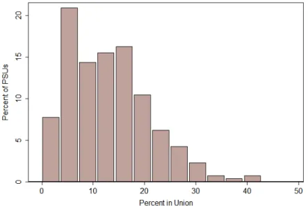
The variation in health insurance by PSU may be due to a variety of factors. One possibility is the level of penetration of workers’ unions in a PSU. Unions may have more power in negotiating health insurance directly from an insurer or through a firm for their members and a location with a higher frequency of labor union membership may mean lower health insurance premiums in general. Figure 5.3 presents a histogram of the percentage of individuals who are members of a workers’ union by PSU. A simple regression of union penetration on the percent uninsured in a PSU shows that union status is statistically correlated with higher percentages of insurance across PSUs (P −value = 0). However, union status maybe simply be picking up the level of employment in each PSU. Including the employment rates of each PSU in the regression did not make union penetration insignificant. I use the health insurance percentages as instruments instead of union status because PSU level insurance may also pick up other characteristics of each location, such as local laws affecting insurance companies’ presence and/or their premiums (Rizzo and Zeckhauser, 2005).
Figure 5.1: Variation in Insurance by PSU
Figure 5.3: Variation in Union Penetration by PSU
Chapter 6
Results and Simulations
6.1
Goodness of Fit
The preferred specification is a joint estimation of the demand and production equa-tions defined in Chapter 5 that accounts for the presence of unobserved heterogeneity and its correlation across equations.
To assess that the model fits the data well, Table 6.1 compares means predicted from the model with actual means from the summary statistics in Table 4.3. Dependent variables are predicted with the estimated coefficients each period and then used to update the endogenous explanatory variables in the next period. In the first period, the predicted value of initial health is used to update health in the insurance, diagnostic and input behavior equations. The means are very similar, demonstrating that the model fits the means of the actual data rather well. A χ2 goodness of fit test (also known
as a Pearson’s χ2 test) tests the null hypothesis that the frequency of occurrence of
an event in the actual and observed samples are from the same frequency distribution. The test statistic isχ2 =Pn
i−1
(Oi−Ei)2
Ei whereOi andEi are the observed and expected
frequencies. The statistic is drawn from a χ2 distribution with two degrees of freedom
known). None of the calculated test statistics are anywhere near the range in which the null hypothesis can be rejected.
Table 6.2 shows the distribution of the permanent unobserved heterogeneity. The mass points are normalized to be between 0 and 1. The other mass points are estimated to fall at 0.3 and 0.6, with most of the probability falling on 0.3.
In the next section, I show key results from the preferred model. For comparison, I include results from a two-stage least squares instrumental variable approach and a simple model where all explanatory variables are treated as exogenous. A full listing of estimation results is provided in the Appendix.
6.2
Empirical Findings
6.2.1
Insurance Effects
In this section I describe the marginal effects of insurance with drug coverage on diagnostic and medical care and lifestyle behaviors for three specifications: the preferred model (labeled Joint); the two-stage least squares instrumental variables approach (labeledIV); and a simple model where each equation is estimated independently with logit specifications (labeled Exogenous).
Marginal effects for discrete outcome models are more complicated than for contin-uous outcomes. For a logit model where
P(Y = 1) = logit(β1x1+Xβ), (6.1)
the effect on Y, the outcome of interest, of a one unit change on x1 is not simply
β1 as would be the case with a continuousY. Instead, the marginal effect is the effect
onP(Y = 1) of a discrete change in x1 and is written as
∆P(Y = 1) ∆x1
= exp(β1+Xβ) 1 + exp(β1+Xβ)
− exp(Xβ)
1 + exp(Xβ). (6.2)
for binaryx1. The marginal effect ofx1 depends on the value ofX andβ. In evaluating
the marginal effect, I leave all other x’s besides x1 at their observed values. Standard
errors are bootstrapped using 500 draws.
The IV model requires the estimation of two stages. Because each stage involves discrete outcomes, I cannot run logit regressions in each stage and simply use the predicted value from the first stage in the second stage. Instead, I treat insurance as a binary variable use a linear probability model in the first stage and include the predicted residual in the second stage. The standard errors are bootstrapped with 500 draws.
Table 6.3 lists the marginal effects of insurance with drug coverage compared with no insurance on each of the diagnostic care and input behavior variables. Considering the Exogenous model first, insurance with drug coverage is associated with an increase in the probability of seeking diagnostic care, ranging from an 8 percent increase in seeking a foot exam to a 14 percent increase in the probability of obtaining a blood glucose exam. However, these results are misleading, as it is likely that sicker individuals seek more diagnostic care and are also more likely to purchase insurance. Not accounting for this self-selection into insurance plans will lead to an upward bias on the effect of insurance. The Joint and IV framework address this problem by using instruments that affect insurance selection, but do not affect medical care to predict insurance, purging the variable of endogeneity. In the IV specification, the presence of insurance is regressed on market-level insurance characteristics and other exogenous variables in the first stage. In the second stage, the health inputs are estimated using the predicted residuals for insurance.
the Exogenous estimates, indicating that adverse selection is present. That is, failure to account for the adverse selection yields parameter estimates that are biased upwards. However, the IV results are all insignificant. The Joint estimates are generally larger than the IV estimates and are significant for the diagnostic care variables. Using a Hausman specification test, I compare the Joint and IV models. I test that the consistent IV specification differs from the Joint model, which is assumed to be efficient. The test statistic is H = (βc −βe)0(Vc −Ve)−1(βc −βe) where c denotes consistent,
e indicates efficient and V is the variance of each estimator. I find that none of the resulting Chi squared distributed statistics are significant at any traditional significance levels, indicating that the IV model does not contain any additional information not in the Joint model i.e., the Joint model is also consistent. The Joint estimation is preferred as it allows for the unobserved characteristics to affect each equation through a permanent heterogeneity term.
The effects of drug coverage on diagnostic care and input behaviors are shown in Table 6.4. Not surprisingly, the coefficients are mostly insignificant due to the small number of people in the sample who are insured without drug coverage.
6.2.2
Health Production
The health production equations include interactions between lagged health and health inputs (both discrete variables). The marginal effect an interacted variable must account for the additional term. For a logit model where
P(Y = 1) = logit(β1x1+β2x2+β12x1x2+Xβ), (6.3)
the marginal effect ofx1 on P(Y = 1) is now
∆P(Y = 1) ∆x1
= exp(β1+β2x2+β12x2+Xβ) 1 + exp(β1+β2x2+β12x2+Xβ)
− exp(β2x2+Xβ) 1 + exp(β2x2+Xβ)
. (6.4) Table 6.5 reports the marginal effects of health inputs on health outcomes from the Joint, IV and Exogenous approaches. In the IV estimation, health, measured by the presence of eye and kidney problems, is estimated in the second stage. The first stage consists of diagnostic, medical and lifestyle behaviors regressed on insurance, education and other socio-demographic variables. Since insurance is endogenous, I include the instruments for insurance instead of insurance in the first stage.
The estimates from the exogenous model on diagnostic care and input behaviors are generally the incorrect sign, which is consistent with biases attributed to the en-dogeneity of health inputs. The IV and Joint estimations correct for this enen-dogeneity, but once again the IV estimates are insignificant. In both the IV and Joint estima-tion, the probability of an eye problem generally decreases with diagnostic care and input behaviors. From the Joint model, diagnostic care decreases the probability of eye problems by up to three percent by seeking a blood glucose exam at least twice in the last year, though checking blood pressure in the last three months did not appear to affect the probability of an eye problem. Lifestyle changes are associated with a drop in the probability of eye problems in both specifications, but the IV estimates are several orders larger and insignificant. Using oral medications for diabetes treatment significantly lowers the probability of an eye problem by almost four percent in the Joint estimation. The results on the probability of kidney problems are similar, though obtaining an HBA1c test at least twice a year does not appear to be associated with a lower probability of kidney problems.
Joint model is correct. In addition, the IV estimates do not account for any hetero-geneity in individuals not captured by observed covariates. For example, an unobserved preference for self-protection that is omitted from the IV equation would bias the es-timates on lifestyle behaviors upward (a larger negative number in this case), since the positive health effects of self care would be captured by the variables that are also affected by unobserved self-protection preferences. Table 6.6 lists the coefficient, ρ, on the unobserved heterogeneity term,µ, for each of the jointly estimated equations. The coefficient is negative and significant in the health equations (except in the comparison of good health with excellent health, but this is a self-reported measure and the differ-ence between very good and good health may not be so distinct). It is also negative and significant in all the diagnostic equations. This is consistent with the existence of an unobserved preference for self-protection that decreases the likelihood that the in-dividual seeks diagnostic care, but positively affects health. The coefficient onµis also negative on the lifestyle behaviors, which is counterintuitive with µ as an unobserved preference for self-protection. However, the coefficients are small and insignificant on exercise (and significant at the 10 percent level on diet only), but larger and signifi-cantly different from zero on the use of medications, even in conjunction with diet and exercise, which is consistent with an aversion to formal care.
6.3
Health Insurance Simulation
In order to capture the full effects of insurance on health, I simulate three cases using the results from the Joint model: (1) all individuals are uninsured; (2) all individuals are insured without prescription drug coverage; and (3) all individuals are insured with drug coverage. For each case, the simulation is performed by using predicted outcomes from the estimated coefficients every period to update the endogenous explanatory
variables in the next period.
Columns (1) through (3) of Table 6.7 list the percentage of individuals who engage in each activity under each insurance scenario from simulations of the model. The fol-lowing three columns report percentage point changes between the insurance scenarios. The presence of insurance coverage without drug coverage (Column (2)-(1)) increases the probability of obtaining diagnostic care compared with no insurance. The proba-bility of obtaining a cholesterol test increases by 14 percentage points and is the only change that is significant. The probability of exercising decreases by nine percentage points indicating that some amount of moral hazard may exist, but this value is not significant. As expected, the probability of using oral medications decreases. Column (3)-(2) reports the effects of drug coverage (conditional on insurance coverage). None of the values are significant and the probability of an eye and cholesterol exam de-crease with the drug coverage. The last column reports the total effect of insurance with drug coverage on these health behaviors. The probability of obtaining each of the diagnostic check-ups increases by at least six percentage points and are all significantly different from zero. The probability of modifying the diet increases by eight percentage points and is significant at the 10 percent level, indicating that individuals do allocate resources to this lifestyle behavior.