The Effects of Body Size on Electability
By Tisha Martin
Senior Honors Thesis Political Science
University of North Carolina at Chapel Hill
April 2nd 2018
Approved:
Thesis Advisor
Reader
TABLE OF CONTENTS
INTRODUCTION………... 3
CHAPTER ONE: AN INVESTIGATION OF REPRESENTATION AND BIASES………... 9
Substantive Representation, Descriptive Representation, and Body Size……... 9
A Lacuna in the Existing Knowledge about the Effects of Body Type………… 15
CHAPTER TWO: HYPOTHESIS……… 21
CHAPTER THREE: RESEARCH DESIGN………... 22
CHAPTER FOUR: DESCRIPTIVE STATISTICS……… 28
Figure 4.1: Age………. 28
Figure 4.2: Gender……… 30
Figure 4.3: Party Identification………. 31
Figure 4.4: Household Income……….…. 32
Figure 4.5: Highest Level of Education……… 33
Figure 4.6: Measure of Attention……….…. 34
Figure 4.7: Political Knowledge Index………. 35
Figure 4.8: Index of Political Participation………... 36
Figure 4.9: BMI of All Respondents……… 38
Figure 4.10: BMI……….. 39
CHAPTER FIVE: RESULTS AND IMPLICATIONS………... 40
Table 5.1: Guessed Weight of the Candidate as a Manipulation Check………... 41
Table 5.2: Main Effect of Candidate Body Size on Character Judgments…….. 43
Table 5.3: Gender as a Moderator for the Effects of Candidate Body Size…….. 45
Table 5.4: Gender as a Moderator for the Effects of Candidate Body Size…….. 47
Table 5.5: BMI as a Moderator for the Effects of Candidate Body Size……….. 50
Table 5.7: Political Participation as a Moderator of the Effects of Candidate Body Size……… 55
CHAPTER SIX: CONCLUSION………... 60
INTRODUCTION
In 1965, a woman who knows that she is a size twenty, and spending her day
shopping at Macy’s, could pick up several different items of clothing from several
different brands and happily purchase them without having to try them on. She can even
go across the street to JC Penny and do the exact same thing. She knows that she wears
one of the biggest sizes in the store, and may feel a little self-conscious about having to
pick items from the back of the rack due to society’s unwarranted beauty standards, but at
least she knows that the items that she has purchased will fit when she go to wear them.
However, things are not so simple in 1975. She goes into Macy’s to purchase a
dress for her night out, goes home, pulls off the tags, and attempts to put it on only to find
that it does not fit! She checks the tag to make sure that it is a size twenty, and even step
on the scale to see if she has gained a few pounds since the last time she went shopping.
The dress is certainly a size twenty and she has not gained an ounce, so why does the
dress not fit? She has some time to spare, so she throws something else on, hops into her
car, and goes the neatest department store. She grabs three different dresses, all a size
twenty, and struggles to find the dressing room that she has never had to use before. None
of these dresses fit either. So she has to walk out of the store empty handed and drive
across town to another department store in hopes of better luck. She arrives, grabs three
dresses, all of them a size twenty, and rushes to the dressing room. Only one of them fits,
and it happens to be her least favorite one. She purchases it anyway and rushes back
six dresses, all claiming to be a size twenty, she could only manage to fit into one! Why
has shopping become so difficult for her?
Shopping was easier in 1965 because the National Bureau of Standards, which is
now referred to as the National institute of Standards and Technology, enforced sizing
regulations that told clothing manufactures the exact measurements for every available
size. If you wore a size twenty in Levis, then you knew that you wore a size twenty in
every other brand available in the United States as well. However, the National Bureau of
Standards declared their sizing regulations voluntary in 1970, and the federal government
completely withdrew the standards in 1983 (Felsenthal). While overturning sizing
regulations had a few positive consequences, such as a wider variety of clothing sizes that
account for various body shapes, it also had the unintended consequence of making
shopping harder for those near the ends of the sizing spectrum. Additionally, it
contributed to the birth of vanity sizing, which is the practice of sizing clothes to be
larger than the average article of clothing claiming to be that particular size. This practice
can leads to individuals feeling shameful when they shop at a store that does not use
vanity sizing because they have to purchase a larger size at such stores. Congress could
have taken steps to stop this change. After all, Article 1 of the Constitution vests in
Congress the power to, “fix the Standard of Weights and Measures,” and as such it
oversees agencies such as the National Bureau of Standards. However, Congress took no
action. In fact, these standards dissolved without much consideration as to whom it may
affect. Why would Congress not exercise its ability to set standards in a policy domain
The case of sizing standards for clothing would be easy to dismiss if it were a
one-off episode, but the overturn of sizing regulations is but one instance of a bigger
problem. Both those who are considered under and overweight have to pay more for life
insurance and, before the Affordable Healthcare Act of 2010, health insurance. I must
note that the Affordable Healthcare Act of 2010 is being called into question in the
current political environment, which leaves the potential for those who are under and
overweight to be forced to pay more for health insurance again. In addition, airline
regulations often require people above a certain weight to buy two plane tickets when
they fly. Furthermore, overweight people are less likely to be hired than someone of
average size (Phul and Heuer, 2009). Members of congress could at least start a
conversation about fixing these problems. After all, it is within their power to regulate
life and health insurance agencies, airlines, and discriminatory hiring practices. However,
they did not, which leaves this large group of people misrepresented.
These observations illustrate that, just as Blacks, Latinos, women, and members
of the LGBTQ+ community represent politically significant groups, so too do under and
overweight people represent a political class with joint interests. They have an interest in
health care and life insurance policies that do not punish their weight, airline regulations
and mandates that allow them to fly without having to buy an additional ticket, and
policies that prevent hiring discrimination against them. Additionally, they are affected
greatly by these interests not being tended to, and might organize to accomplish such
policy implementations. Furthermore, there is reason to suspect that under and
overweight Americans, as a political class, are hindered by their lack of descriptive
or super models. Nevertheless, few of them appear to be on the extreme ends of the body
type spectrum, where they experience the hassle of having to purchase two plane tickets
every time that they fly or unnecessary trouble when shopping for clothes such as the
situation above illustrates. This deficit is striking, given that 32.5% of the U.S. population
are considered overweight, and 37.7% are considered obese (NIH 2017).
My research sets out to investigate the possibility that the reason for the lack of
descriptive, and therefore, substantive, representation of those on the extreme ends of the
body size spectrum is a voter bias. Bias at the voting booth is a given. Some biases are
healthy and welcomed, such as a preference for experienced candidates over amateurs.
However, some biases are problematic and leave groups of people improperly
represented, such as the bias against women or candidates of color. Since many of the
problems that overweight and underweight citizens face indicate that they are being
improperly represented, I theorize that my research will find a bias against candidates
with other-than-average body types at the voting booth.
Although my study will have limited applicability to short-term policymaking, it
can generate evidence that speaks to long-standing questions. One goal of my research is
to make voters aware of this potential bias and therefore, able to prevent it from clouding
their judgment of a candidate. If voters are aware that they may have an unintentional
bias against candidates that are larger or smaller than the ideal norm, then my second goal
will be accomplished: they are likely to make attempts to look past such features in order
to better judge a candidate’s ideas and qualifications. If enough people do this, then we
could see more variety in the body types of elected candidates. This will mean that my
the current system will have a chance to make positive changes. Such could lead to a
rebirth of sizing regulations that account for the variety of body sizes represented in the
U.S., laws protecting the discrimination of overweight job applicants, a minimum size for
airplane seats, and lower rates for life insurance for those with an other-than-average
body size.
This thesis starts with a chapter on past research concerning descriptive
representation, substantive representation, and voter biases based on appearance. This
chapter provides insight into why voter biases matter for the descriptive representation,
which often leads to substantive representation, by discussing its importance to other
groups often left out of the political arena. Then, this chapter makes a case for why
descriptive representation may help those with other-than-average body sizes like it has
been proven to help other similar groups. Lastly, this chapter explores studies that helped
me formulate my hypothesis. These studies feature the effects of attractiveness on
character judgments and the likelihood that a candidate will receive votes, what features
contribute to these appearance-based character judgments, and how factors such as
gender and political sophistication moderate these appearance-based character judgments.
Chapter two simply states my hypothesis, which is that candidates with an average body
size will be judged more favorably and more likely to receive votes than those with an
above or below average body size. Chapter three features a detailed description of my
research design and an overview of how I analyze the data gathered from my survey
experiment. Chapter four includes descriptive statistics in the form of histograms. These
histograms serve the purpose of detailing the demographics of who participated in this
the results reported in the tables, and potential implications for the significant findings.
CHAPTER ONE: AN INVESTIGATION OF REPRESENTATION AND BIASES
I. Substantive Representation, Descriptive Representation, and Body Size
Descriptive and substantive representation are very important terms for discussing
political minorities. Descriptive representation describes having a representative that
looks and identifies the same as the elector. A black representative provides descriptive
representation for blacks, and a representative who is a woman provides descriptive
representation for women. Substantive representation describes having a representative
who promotes policies that benefit the political class to which that the elector belongs. A
representative who supports policies that benefit women provides substantive
representation to women, and a representative who supports policies that benefit Latinos
provides substantive representation to Latinos. Substantive representation can occur
regardless of how the representative looks or identifies. A white representative can
provide substantive representation for racial and ethnic minorities, and a representative
who is a man can provide substantive representation for women. This is true because
substantive representation, unlike descriptive representation, concerns policies
introduced, sponsored, or endorsed by the representative. While descriptive and
substantive representation are different, there is a lot of debate concerning the
relationship between the two. Such debate concerns questions such as how important is
descriptive representation, for substantive representation? Also, can you have the latter
without the former? Studies of African Americans’ political interests provide one set of
answers.
Carol Swain in Black Faces, Black Interests sets out to distinguish between blacks
starts by examining how well congress as a whole represents black interests, and
determines what is considered black interest by looking at the poverty rate and housing
conditions for blacks, the preferences of black interest group leaders, and the preferences
of blacks as a whole. Then she looks into how individual congressional members behave
in order to determine whether or not descriptive representation of blacks actually leads to
the needs of blacks being met. She finds that party matters more than race; Democrats
aided black interest, not necessarily black representatives. From there she argues that
attempting to increase descriptive representation can actually lead to less substantive
representation on account of the methods used to accomplish this goal. The method that
she focuses most on is the drawing of majority-minority districts, which she argues often
creates more majority-white districts and leads to more Republicans in congress on
account of whites being more likely to vote for Republicans. Swain also notes that the
Congressional Black Caucus lost power when Republicans became the majority. Since
having Democratic representative tends to promote the interests of blacks more so than
simply having black representatives, she gathers that factors such as campaign finance
hold blacks back from increasing their political power instead of a lack of descriptive
representation (Swain 1993). She is not alone in questioning the importance of
descriptive representation for blacks.
Katherine Tate questions how helpful descriptive representation is for blacks in
Black Faces in the Mirror. She uses data gathered from a 1996 National Business Ethics
Survey (NBES) in order to make her claim. The survey results find the following: blacks
are no more or less satisfied with congress as a whole than whites, blacks are no more
gained by a black representative diminishes after a while. She uses this data to argue that
descriptive representation is not always helpful or needed for the promotion of black
interests. However, the NBES results do indicate that descriptive representation is helpful
for blacks under certain conditions, such as the plurality electoral system present here in
the United States. While having a black Senator did not make blacks more likely to know
the party identification of their Senator, having a black House Representative did make
blacks more likely to know this information. Additionally, having a black Senator or
House Representative made blacks more likely to know the official’s name. Lastly, 60%
of blacks support electoral reform that will increase their descriptive representation in
Congress, which means that it matters a great deal to the black community. Essentially,
Tate is not outright denying the usefulness of descriptive representation, but is arguing
that it is not always helpful under every possible set of conditions and cannot be used as a
simple “cure” for all of the political troubles that blacks face (Tate 2004). Swain and Tate
argue that descriptive representation for blacks does not always lead to substantive
representation. However, this does not mean that descriptive representation never leads to
substantive representation.
Gerrity, Osborn and Mendez found that representatives who are women are more
committed than men when it comes to sponsoring bills that benefit women’s issues. The
researchers define women’s issues broadly in terms such as women’s health and equality
within the work place (Gerrity et al. 2007). Kerr and his team of researchers found that
having a black mayor leads to an increase in administrative jobs for blacks in that
municipality. Additionally, an increase in Latino council members leads to an increase in
that constituents are more likely to communicate with their representative if that
representative is of the same race of them. He focused on blacks and whites for this study
(Broockman 2014). Being more or less inclined to communicate with one’s
representative matters because it is an indicator of political engagement and participation.
Additionally, representatives do not work to solve problems that they do not know about,
so being more or less inclined to communicate with your representative can affect one’s
substantive representation. Lastly, Wald, Button, and Rienzo found that openly gay
candidates running for office leads to more anti-discrimination ordinances within that
municipality (1996). These studies show that there are substantive gains from descriptive
representation for several different minority groups in at least some cases. While the
work done by Swain and Tate show that there is still debate regarding this matter for
African Americans, there is less debate for other minority groups.
Walter Clark Wilson makes the case that Latinos represent the interests of Latinos
more effectively than non-Latinos in From Inclusion to Influence. Latino representatives
are able to allow for the inclusion of Latinos in politics, connects Latinos to the
government, introduces Latino concerns, and allows Latinos to shape public policy.
Additionally, the inclusion of Latinos allows for a better democracy by expanding who is
welcomed inside the political arena. While some scholars, such as Swain, claim that party
identification matters more than race for the substantive representation of blacks, Wilson
argues descriptive representation can lead to substantive representation no matter what
party a representative belongs to for Latinos. In fact, Wilson argues that having Latinos
on both sides of the aisle and in a wide range of committees is actually best for Latino
in the real Latino population to be reflected in Congress. To further explain this point, he
points to three Latino representatives: Robert Menendez (D-NJ), Marco Rubio (R-FL),
and Ted Cruz (R-TX). These three representatives are from both the Democratic and
Republican party and disagree on at least a few policy points. However, so do members
of the Latino population in general. Additionally, while they disagree on most policy
measures, they agree on key issues concerning immigration and civil rights that are
included in the broad definition of Latino interests (Wilson 2017).
Another example that Wilson provides involves former Representative Joe Baca
(D-CA) who was on the Agricultural Committee during the 100th Congress. While there,
he was able to address the interest of Latino Farmers, who dominate the Southwest, when
Congress renewed the Farm Bill. Having Baca on the agricultural committee did not
necessarily help Latinos in the Southeast and other regions of the country. Even so, it
advanced the interests of the Latino farmers located in the Southwest, which is still a
Latino interest (Wilson 2017). Descriptive representation seems to be just as helpful for
women as well.
Michele Swers argues that descriptive representation leads to substantive
representation for Women in The Difference Women Make. She uses evidence gathered
from a quantitative analysis of bills, interviews, and members of the representative’s staff
in order to make her claim. While representatives who are women often vote along party
lines, their gender still matters in their decision making. Additionally, political context
affects how aggressively women advocate for women’s issues. Even so, representatives
who are women do a better job of representing women than their male counterparts
value to having descriptive representation for women (Swers 2002). Descriptive
representation seems to not always be of much use to blacks, but it seems to greatly
benefit Latinos, members of the gay community and women. Such leaves a question
regarding how helpful descriptive representation will be for those with
other-than-average body sizes.
Descriptive representation is likely to lead to substantive representation for those
with other-than-average body sizes on account of their similarities to Latinos and women.
Blacks tend to be more uniform in thought. As Swain points out, this causes them to be
better represented by a party than an individual representative. This is the biggest reason
why descriptive representation is less likely to lead to substantive representation for
blacks (Swain, 1993). However, as Wilson points out, Latinos are less uniform in their
political ideology and policy needs. They seem to only be uniform on a few key issues
concerning immigration and civil rights. This makes having Latino representatives matter
more so than having a representative with a particular party identification. Additionally, it
is why having Latinos on both sides of the aisle and on a wide range of committees is
very beneficial for the Latino community here in the United States (Wilson 2017). Swers
argues that descriptive representation leads to substantive representation for women, and
it is likely for similar reasons (Swears 2002). Women are arguably the least uniform
minority group, only agreeing on a small set of issues such as child care. Those with
other-than-average body sizes are likely to share the diversity experienced by Latinos and
women that causes descriptive representation to matter more than party in creating
Those with other-than-average body sizes are not necessarily confined to one
region, socioeconomic class, race, religion, political party, etc. Additionally, they lack a
tight-knit community with shared customs and values. Even so, they have a small set of
issues that they are likely to agree on, such as health care and life insurance. This sounds
very similar to the way Wilson and Swers describe Latinos and women (Wilson 2017,
Swears 2002). If descriptive representation does not always lead to substantive
representation of blacks on account of their uniformity, and descriptive representation is
more likely to lead to substantive representation for Latinos and Women on account of
their lack of uniformity, then it follows that lacking uniformity is a major component in
descriptive representation leading to substantive representation. Those with other-than
average body sizes clearly lack this uniformity, for reasons stated above, so they are
likely to gain substantive representation from descriptive representation.
II. A Lacuna in the Existing Knowledge about the Effects of Body Type
People tend to judge the traits of others, such as attractiveness, competence,
approachableness, and trustworthiness, by their appearance. Belot, Bhaskar and Ven
studied the dynamics of the game show “Does (s)he share or not?” and found that, while
players who are considered unattractive preform no better or worse than their peers who
are considered attractive, they are far more likely to be eliminated from the show by their
fellow contestants. Participants in this study accurately predicted that attractiveness
played a role in a player’s likelihood of winning, however, they greatly underestimated
the magnitude of this role and were shocked by the results of the study (Belot 2012).
Several researchers have found that these judgments are extended to electing candidates
captain of their boat matched the results of adults who believed that they were selecting a
political candidate based on competence (2009). These findings are consistent with the
findings of several other scholars that suggest that the electorate make appearance-based
judgments regarding traits such as competence and trustworthiness.
Atkinson and Hill collected data on the facial competence of 972 candidates and
used that data when creating their survey experiment to measure the effects of appearance
on the outcome of elections. They found that “face quality” had an effect of 4 percentage
points for independent senate challengers and 1-3 percentage points for partisan senate
challengers. The researchers controlled for the representative’s political party when they
found the 1-3 percentage point effect for partisan senate challengers. This difference may
matter in a very close election, but did not decide any of the 99 senate elections in the
study (Atkinson 2009). Mattes showed his subjects two photos and asked them to judge
the faces in the photos in terms of competency, attractiveness, deceitfulness and how
threatening they looked. The researchers found that the more threatening a candidate
appeared, the less likely they are to win. They also found that attractiveness yielded a
negative correlation with electoral success when paired with incompetence. Lastly, they
found that competence was positively correlated with electoral success. This suggests that
competence matters more than attractiveness, but attractiveness still plays a role (Mattes
2010). Todorov and his team had their participants rate U.S. Senate candidates based on
competence, which they inferred from attractiveness. They found that facial appearance
predicted 68.8% of senate races in 2004. The judgments made by the participants on how
competent the candidates appeared happened within one second of exposure to their
and matter more when the election focuses on the candidate as an individual instead of
the party that he/she belongs to (Lawson 2010).
Lawson, Myers, and Baker asked American and Indian subjects to rate the faces
of Brazilian and Mexican candidates shown in black and white photographs. The ratings
gathered in the study matched actual election results for Mexico and Brazil. Additionally,
they found that the correlation was strongest in Mexican gubernatorial and presidential
elections, which are decided by plurality-winner rules, and weakest in other elections that
rely on an electoral system that promotes stronger party line voting. This suggest that
voters are using appearance as a way to compensate for actual information on political
candidates (Lawson 2010). Other scholars have found results that seem to suggest the
same thing. Banducci, Karp, Thrasher, and Rallings Researched a set of elections where
the electorate was provided with little information on each candidate and photographs
were present on the ballot. They found that the electorate used physical appearance to
decide who to vote for, and that candidates who were perceived as being more attractive
are also perceived as having qualities that make them more capable of leadership
(Banducci 2008). However, other studies have found that even the politically
sophisticated are guilty of making voting decisions based on appearance-based
judgments. Brusattin asked participants questions that allowed him to determine their
level of political sophistication based on their political knowledge and participation.
Then, he presented them with two hypothetical candidates with detailed policy statements
attached. On average, participants chose the most attractive candidate, regardless of the
soundness of their policy statement. This is true for the politically sophisticated
study seems to suggest that members of the electorate are not simply using appearance as
a heuristic.
The preferences of character traits derived from appearance-based judgments
differs based on the gender of the candidate and the electorate. Chiao, Bowman, and Gill
asked their participants to rate candidates based on how dominant, compentet attractive
and approachable they seemed. These ratings were based on the candidate’s facial
appearence. They were then asked to pick a candidate for a hypothetical presidential
election. They found that, men tend to vote for attractive female candidates. In contrast,
women tend to vote for approachable male candidates (Chiao 2008). Such suggest that,
while we all make character judgments based on appearances, we differ on which
character judgments appeal to us. For this reason, it is important to measure differences
across demographics. However, all of the studies mentioned above all assume that these
judgments are based on facial features.
For all their strengths, a commonality across the studies reviewed above is that
they take a narrow view of what constitutes attractiveness. In particular, they focus only
on facial features. This could be an important shortcoming considering that more than
facial features often goes into our evaluations of attractiveness. We often consider factors
such as one’s demeanor, dress, and build as well when making judgments regarding
attractiveness. Spezio and his team came across a small aspect of this intersectional
approach to evaluating attractiveness during their study (2012).
While the researchers discussed previously have, for the most part, assumed that
facial features provide the cues that the electorate base their appearance-based judgments,
Gosselin, Mattes, and Alvarez had participants look at pictures and decide who looks
more or less threatening, who looks competent enough to hold office, and who they
would be likely to vote for. When the participants only looked at the candidates faces,
there was no significant relationship between their decisions and actual election results.
However, when they removed the faces from the images and showed more of the
candidate’s body, a strong positive relationship existed for all judgments the participants
made. Ultimately, this study shows that body type has a significant impact on the
appearance-based character judgments that members of the electorate make. The body
type of the candidate may even have a larger impact on the appearance-based judgments
of the electorate than the candidate’s facial features. Although, the researchers do not go
into detail about what body features led their participants to make the judgments that they
did, or the impact of individual body features on these judgments (Spezio 2012).
The studies above agree that people make character based judgments based on
appearance. Such character judgments include how competent, trustworthy, and
approachable one is. Additionally, we tend to carry these appearance based character
judgments into the voting booth. While we can predict the outcome of elections based on
the findings above, most scholars do not believe that these appearance-based character
judgments actually decide elections (Atkinson 2009, Mattes 2010). Furthermore, these
appearance-based character judgments exist across cultural boundaries and matter more
when the focus is on the candidates as individuals instead of their party (Lawson 2010,
Banducci 2008). While this suggests that voters are using appearances as a heuristic, such
us contradicted with findings that even the politically sophisticated fall victim to these
these appearance based judgments came from facial features. However, Spezio and his
team found that aspects other than facial features play an important role in these
judgments. Even so, they did not measure the effect of specific features to determine their
impact (Spezio 2012). My study, while inspired by the ones mentioned above, plans to go
beyond existing research.
My research can contribute to the collective knowledge about factors affecting
electability by focusing on a narrow and clearly measurable feature, which is body size.
As mentioned previously, most of the studies above assumed that their participants were
using facial features in order to make their appearance-based judgments. Spezio’s
findings contradicted this, but his team did not measure the impact of specific features
(2012). Since body size plays an important role in determining the attractiveness of an
individual, I believe that it will also play an important role in appearance-based character
judgments. That is why my study will focus exclusively on the effects of body size on the
electability of candidates to office. Since it is unclear whether or not political
sophistication has an effect on whether or not one is likely to make appearance based
character judgments of a candidate, my study will measure the effects of political
participation and knowledge as a moderator for the effects of a candidate’s body size. My
study will measure political knowledge and participation as separate moderators for the
effects of candidate body size on appearance-based character judgments in order to
CHAPTER TWO: HYPOTHESIS
I hypothesize that a candidate with an average body size will be judged more
favorably and more likely to receive votes than one with an above or below average body
size. This is likely because, as the research discussed previously shows, voters are more
likely to think favorably of a candidate that they find attractive. Body size can be an
indicator of attractiveness, and people tend to favor those with an average body-size.
Therefore, the candidate with an average body size is likely to be thought of more
favorably and receive more votes. If this hypothesis happens to fail, I believe that it will
be because members of my mock electorate are voting for the candidate that corresponds
to their perceived body size. This means that a voters who perceives themselves as being
overweight will be more likely to vote for an overweight candidate, those who perceive
themselves as being of an average body size will be more likely to vote for a candidate of
average body size, and those who perceive themselves as being slender will be more
likely to vote for a slender candidate. This will likely be the case if my hypothesis fails
because people tend to vote for those who they can relate to the most. When relying
almost solely on a photograph, the mock electorate will try to find ways in which the
mock candidate is relatable through his appearance. With all things controlled for except
for body size, it is likely that the mock electorate will use that as a primary cue to decide
if they would vote for the mock candidate or not. However, I only expect the latter to
CHAPTER THREE: RESEARCH DESIGN
I tested the hypothesis stated in chapter two using a survey experiment crafted in
Qualtrics. The respondents were from Amazon Mechanical Turk and paid fifty cents for
participating in this survey, which took approximately eight minutes to complete. Only
people over the age of 18 and residing in the United States were able to view my survey
on the platform. The survey received roughly 430 responses, although not all of the
respondents fully completed the survey. Amazon Mechanical Turk is a convenience
sample given that it provides a sample that is not exactly representative of the United
States. Such lead to my sample not being truly randomized; however, the study and the
results are still useful. While this is not a sample truly representative of the U.S.
population, it is still a decent sample and can still clue us in on whether or not there is a
bias against those with other-than-average body sizes.
The survey began with a standard consent form informing the participants of their
rights, what they will be paid for taking the survey, a brief overview of what will be
asked in the survey, the IRB study number, and necessary contact information. Next the
participants were asked, “How old are you?” The options were, under 18, 18-24, 25-34,
35-44, 45-54, 55-64, 65-74, 75-84, 85 or older. If a participant selected under 18, then
that participant was automatically directed to the end of the survey. This was done in
order to prevent those who are under 18 from participating in the study. Next, participants
were asked about their political ideology. They were asked, “Where would you place
yourself on this scale?” The options were a 7-point Likert scale ranging from extremely
liberal to extremely conservative. Afterwards, the respondents were randomly assigned to
sized candidate, or below average sized candidate. This was the beginning of their
judgment task.
The photos presented to the participants were exactly the same aside from the
candidate’s body size. Each photo also featured a short platform regarding the politician’s
imagined candidacy to the participant’s local school board. It read as follows:
“Imagine that this man is running for a seat on your local school board. He is a
proud parent of a student in the district and knows the true value of education. He
is a dedicated parent who participates in community fundraisers and is a member
of the PTA. If elected, he will make sure that every child has what is necessary to
succeed and will promote education policies that will work for everyone.”
This platform is very neutral and agreeable, and was below each photograph in order to
control for any potential impact it may have on the study. Additionally, I recorded how
long the participants spent looking at the photograph in order to note which condition
each participant received for the purpose of conducting statistical analyses later in the
study. Featured below are the pictures used in each condition. The first image is the
above average sized candidate, second is the average sized candidate, and last is the
After looking at either the slender, average, or fully built version of the mock
candidate, the participants were asked, “How well do the following words describe the
candidate that you just saw?” The words were competent, threatening, attractive,
trustworthy, and approachable the candidate is. These words were inspired by the
questions asked in the studies mentioned in the second part of chapter one. Their options
were on a 5-point Likert scale that ranged from not at all to extremely. After answering
these questions, the participant were asked how likely they were to vote for the candidate
that they just saw. These options were on a five-point scale ranging from not at all to
extremely, just like the previous questions. Then, the participants were asked a series of
questions regarding their political involvement.
The political involvement questions were presented in a matrix and asked the
follows: during the past 4 years have you telephoned, written to, or visited a government
official to express views on a public issue, joined in a protest march, rally, or
demonstration, contacted or tried to contact a member of the U.S. Senate or U.S. House
of Representatives, attended a meeting of a town or city government or school board,
discussed politics with family or friends? Their options for each of these aspects of
political participation were, “have done this in the past four years,” and, “have not done
this in the past four years.” These answers were used to give participants a political
involvement score, which ranged from 0-5. If they answered that they had done one of
the five activities, then they received a point. If they answered that they had not, then
they did not receive a point for this calculation. Next, the respondents were asked a series
The questions concerning the political knowledge of participants were used to
generate a political knowledge score for the participants. The process for calculating the
political knowledge score is the exact same as the process for calculating the political
involvement score, except that the political knowledge scores range from 0-4.
Respondents were asked, “What is Medicare?” and the options were, “a program run by
the U.S. federal government to pay for old people’s health care,” “a program run by state
governments to provide health care to poor people,” “a private health insurance plan sold
to individuals in all 50 states,” and “a private non-profit organization that runs free health
clinics.” “A program ran by the state governments to pay for old people’s health care” is
the correct answer. Next, they were asked, “do you happen to know how many times an
individual can be elected President of the United States under current laws?” Their
options were 2, 4, 6, 8, and 10. The correct choice is 2. Then they were asked, “Is the
U.S. federal budget deficit –the amount by which the government’s spending exceeds the
amount of money it collects –now bigger, about the same, or smaller than it was during
most of the 1990s?” Their options were bigger, about the same, and smaller. The correct
answer is bigger. Lastly, they were asked, “On which of the following does the U.S.
federal government currently spend the least?” The options were foreign aid, Medicare,
National Defense, and social security. The correct answer is foreign aid. Then the
participants were asked standard demographic questions.
The demographic questions immediately followed the political knowledge
questions, with the exception of the age question, which was placed at the beginning of
the survey in order to exclude those under the age of 18 from participating in the survey.
other. Then they were asked, “What was your total household income in the past 12
months?” with twelve options ranging from less than $10,000 to more than $150,000
with $9,999 intervals. Next, they were asked, “What is the highest level of school you
have completed or the highest degree you have received?” The options were, “did not
complete high school, high school graduate,” “some college, no degree,” “two year
associate degree from a college or university,” “four year college or university degree/
Bachelor’s degree,” “some post graduate or professional schooling, no post grad degree,”
and “post graduate or professional degree, including masters, doctorate, medical, or law
degree.” Then the participants were asked a few questions regarding their body type.
After completing the demographic section described above, the participants were
asked to report their perceived body size. The question was, “Which best describes your
body type?” and the options were, slender/ small, average/ medium, fully built/ curvy,
and bodybuilder. The option “bodybuilder” was included to separate them from the other
categories. Someone who is a bodybuilder or is very muscular may choose fully built/
curvy if the bodybuilder option was not present. However, the fully built/ curvy category
was intended for those who are seen as heavy-set in terms of weight and body-fat. Then
the participants were asked to report their height and feet in inches, and their weight in
pounds. The participants used a sliding scale to answer. Specifically, they were asked,
“What is your height and feet in inches?” and the sliding scale for both feet and inched
ranged from 0-12. Then, “What is your current weight in pounds? If you are above
500lbs, please select 500lbs” and the sliding scale ranged from 0-500. This information
they were asked to, “Attempt to guess the weight of the candidate in this study” and the
sliding scale ranged from 0-500.
Next, the participants were asked a question to make sure that they were paying
attention to the survey. This question read, “If you are paying attention, please select
"slightly unlikely."” The options were on a Likert 7-point scale ranging from extremely
likely to extremely unlikely. Lastly, they are presented with a debrief form on the last
page of the survey. This debrief form reminded the participants of their rights and other
relevant information featured in the consent form, and gave them a summary of the true
intent of the survey.
I analyzed the descriptive statistics for this study using SPSS. These descriptive
statistics can be found in chapter four. I further analyzed the data gathered from the
survey experiment using StataSE, and reported the results in chapter five. These analyses
included a manipulation check using the guessed weight of the candidate that the
respondent was shown, a measure of the main effect of the treatment on the character
judgments and voting decisions made by the respondents, and a measure of the effect of
the treatment on the character judgments and voting decisions made by the respondents
with moderators. These moderators are gender, perceived body size, BMI, political
CHAPTER FOUR: DESCRIPTIVE STATISTICS
This chapter contains descriptive statistics in the form of histograms. These
histograms serve the purpose of detailing the demographic information of those who
participated in this study, and there are ten in total. The wording for questions and answer
choices used to gather this data from the respondents can be found in chapter three, which
details the research design for this study.
Figure 4.1
Figure 4.1 shows the distribution of various ages in my study. The distribution is
the participant is under 18, 2 indicates that the participant is 18-24 years old, 3 indicates
that the participant is 25-34 years old, 4 indicates that the participant is 35-44 years old, 5
indicates that the participant is 45-54 years old, 6 indicates that the participant is 55-64
years old, 7 indicates that the participant is 65-74 years old, 8 indicates that the
participant is 75-84 years old, and 9 indicates that the participant is over the age of 85
years old. The largest category is 25 years old to 34 years old. The smallest category with
values is 75 years old to 84 years old. This could potentially be contributed to the fact
that the instrument was distributed electronically on Amazon Mechanical Turk, which is
more likely to attract younger rather than older people on account of its technological
platform. Younger people are more likely to participate in activities on a technological
platform on account of them being more technologically savvy than older people on
average. Such indicates that there is more representation of young people than older
Figure 4.2
Figure 4.2 shows the distribution of genders for the sample. The exact wording
for this question can be found in chapter three, and the options for gender were “male,”
“female,” and “other.” Male is coded as 0, female is coded as 1, and other is coded as 2.
None of the participants selected “other” and most of the participants were male. The
difference is not that large and should not lead to a problem concerning the
overrepresentation of one gender over another. However, since none of the participants
identify as non-binary or “other,” as it was labeled in the survey, there is a lack of
Figure 4.3
Figure 4.3 shows the distribution of political ideology within the sample. The
exact wording for the question concerning party identification can be found in chapter
three, and the options were a 7-point Likert scale ranging from extremely liberal to
extremely conservative. 1 represents extremely liberal and 7 represents extremely
conservative. There is a slight skew to the left, meaning that most of the participants are
liberal. The smallest category is “Extremely Conservative” and the largest category is
“Liberal.” This skew will lead to liberals being slightly more represented than
Figure 4.4
Figure 4.4 shows the distribution of household incomes for the participants in this
study. There were twelve options ranging from less than $10,000 to more than $150,000
with $9,999 intervals. 1 represents less than $10,000 and 12 represents more than
$150,000. The most represented income bracket is $30,000 to $39,999. Overall, it is
skewed towards the left, which means that most of the respondents are from a lower
income bracket. This skew indicates that those with a lower income bracket will be
Figure 4.5
Figure 4.5 shows the distribution of education levels among the respondents for
this study. The options represented are, “did not complete high school, high school
graduate,” “some college, no degree,” “two year associate degree from a college or
university,” “four year college or university degree/ Bachelor’s degree,” “some post
graduate or professional schooling, no post grad degree,” and “post graduate or
professional degree, including masters, doctorate, medical, or law degree.” The numbers
1-7 represent these options respectively. It is slightly bimodal, meaning that there are two
groups largely represented over others. These groups are those with some college, but no
not finish high school. Therefore, this group, along with the other groups that feature low
numbers, will not have as much representation in this study when compared with those
who have had some college or have obtained a Bachelor’s degree. Education levels are
important for this study, especially concerning political knowledge and participation.
Figure 4.6
Figure 4.6 shows a measure of attention for the respondents in this study. The
exact wording of this question and its options can be found in chapter three. Since it was
a survey experiment, it was very important for the participants to pay attention to their
responses and be deliberate. In order to ensure this, a question was included that simply
featured in figure 4.6. An overwhelming majority of respondents were attentive during
this survey and deliberate with their answers, as indicated above. Such leads to more
accurate results.
Figure 4.7
Figure 4.7 shows the distribution of political knowledge among the participants
for this study. The exact wording for the questions used and their answer choices can be
found in chapter three. There is a very strong skew to the right, which indicates that most
of the participants possess a high degree of political knowledge. Political knowledge was
terms a president can serve and what is Medicare. There were a total of four questions. If
the respondents got a question right, then they received a point. If the respondent got the
question wrong, then they did not receive a point. The sum of their points indicate their
political knowledge index. The maximum points a participant could earn is four, since
there were four questions in total. This strong skew to the right corresponds with the
distribution of education levels among the participants for this study. Since they are more
educated on average, then they are more likely to have more knowledge about the
political system. However, this does not represent the general population since most
members of the general population are not very politically knowledgeable.
Figure 4.8 shows the index of political participation of the participants involved in
this survey experiment. It is skewed left, which means that a lot of people who
participated in this study are not very politically active. Political participation was
measured by asking the participants a series of questions regarding their political activity.
These included questions such as whether or not the participant had voted or contacted a
representative within the past four years. The exact wording for these questions are
featured in chapter three. If the participant answered that they had participated in the
activity in question within the last four years, then they received one point. If the
participant answered that they had not participated in the activity in question within the
last four years, then they did not receive a point. The index of political participation was
calculated by finding the sum of all of the points gained by the participant. The maximum
points that could be earned by a single participant is five. It is not surprising that the
results for political participation are skewed left, considering that matches the trend for
Figure 4.9
Figure 4.9 shows the BMI of all respondents in this study. This figure includes
unrealistic BMI values on account of inaccurate responses by participants. For example,
many participants reported that they were only two inches tall. Such lead to a BMI
calculation of 100,000. The number of responses that reported numbers that lead to these
unrealistic BMI calculations is fairly large. Roughly 46 out of roughly 425 respondents
gave unrealistic responses for their height and weight. Figure 4.10 excluded these
unrealistic responses and therefore, features a more accurate account of the BMI of the
4.10; the lowest height featured in this figure is a little over five feet. Further statistical
calculations including BMI will feature the data shown in Figure 1.10.
Figure 4.10
Figure 4.10 shows the distribution of the BMI among participants for this study,
minus the outliers discussed above. There is a slight skew towards the left; however, this
is because a few respondents have a BMI of 60+, which is not very common in the
general population. Using the scale featured in figure 4.10, the BMI of the general
population would also feature a skew towards the left. For this reason, the skew towards
CHAPTER FIVE: RESULTS AND IMPLICATIONS
As chapter two states, I hypothesize that candidates with an average body size
will be judged more favorably and more likely to get elected than those with an above or
below average body size. If this hypothesis happens to fail, I believe that it will be
because members of my mock electorate are more likely to vote for the candidate that
corresponds to their perceived body size. The numbers shown in the tables below indicate
whether or not the null hypothesis should be accepted or rejected by measuring the effect
of the random assignment of treatment in my survey experiment on the respondents
recruited from Amazon Mechanical Turk. This effect is found by finding the difference in
the means of each treatment group and the control group, then finding the standard error
and level of significance of that difference. All character judgments and how likely the
respondents were to vote for the candidate they were shown were coded from 0-1. “Not at
all” was coded as 0, “slightly” was coded as 0.25, “somewhat” was coded as 0.50, “very”
was coded as 0.75, and “extremely” was coded as 1. All calculations found in the tables
below were found using StataSE and the wording used for the questions in the survey
regarding character judgments and how likely the respondents were to vote for the
candidate that they were shown can be found in chapter three. The first table features the
results of the manipulation check performed to see if the treatments had the desired
effects on the respondents, the second table shows the main effects of the treatment on all
of the respondents as a whole, and the remaining tables feature the effects with various
moderators that are indicated in the title of the table. Note that I did not make any
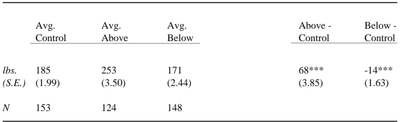
Table 5.1: Guessed Weight of the Candidate as a Manipulation Check
Avg. Avg. Avg. Above - Below -
Control Above Below Control Control
lbs. 185 253 171 68*** -14***
(S.E.) (1.99) (3.50) (2.44) (3.85) (1.63)
N 153 124 148
Note: N = 425, *p<0.05, **p<0.01, ***p<0.001,
Table 5.1 features the guessed weight of the candidate as a manipulation check.
The survey requested that the participants guess the weight of the candidate that they
were shown and this was used to measure the effect of the treatment on the participants.
As expected, the participants guessed a higher weight for the above average sized
candidate and a lower weight for the above average sized candidate when compared to
the average sized candidate, or the control candidate. Note that the average U.S. male
weighs 195.7 lbs. on average (CDC 2017). The average guessed weight for the control, or
average sized, candidate is 185 lbs. This is 10.7 lbs. less than the average weight of a
U.S. male. However, I do not expect this -10.7 lbs. difference to significantly affect my
results because this weight is simply a guess and has room for error. Additionally, the
candidate still looks like he is ofaverage size when compared to the other candidates in
this study. Furthermore, the difference between the average weight of a U.S. male and the
guessed weight of the other candidates in this study is much larger than -10.7 lbs. The
the above average sized candidate is 57.3 lbs. The difference between the average weight
of a U.S. male and the average guessed weight of the below average candidate is -24.7
lbs.
The difference between the guessed weight of the above average sized candidate
and the control is 68 lbs. and the difference between the guessed weight of the below
average sized candidate and the control is -14 lbs. This means that the respondents saw a
notable size difference between the different candidates, and that difference is significant.
Therefore, it appears that the experiment generated the intended perceptions. Even so, the
difference between the effect of the above average sized candidate and the below average
sized candidate must be noted. As the table indicates, the respondents guessed the above
average candidate to be 68 lbs. heavier than the control, and guessed the below average
candidate to be 14 lbs. lighter than the control. That is a 54 lbs. difference between the
effects of each treatment. The smaller effect that the below average candidate had on the
participants could be the reason for the lack of significant results regarding that condition
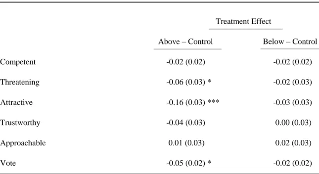
Table 5.2: Main Effect of Candidate Body Size on Character Judgments
Treatment Effect
Above – Control Below – Control
Competent -0.02 (0.02) -0.02 (0.02)
Threatening -0.06 (0.03) * -0.02 (0.03)
Attractive -0.16 (0.03) *** -0.03 (0.03)
Trustworthy -0.04 (0.03) 0.00 (0.03)
Approachable 0.01 (0.03) 0.02 (0.03)
Vote -0.05 (0.02) * -0.02 (0.02)
Note: N=432, *p<0.05, **p<0.01, ***p<0.001, standard error is reported in parenthesis next to the treatment effect, a histogram displaying the number of participants randomly assigned to each condition can be found in table 5.1
Table 5.2 shows the main effect of candidate body size on character judgments.
As indicated, the respondents found the above average candidate less threatening and
attractive. The fact that the larger candidate was seen as less attractive is consistent with
the idea that larger people are less attractive in general. Additionally, the respondents
were less likely to vote for the above average candidate than the control candidate. The
fact that they found the above average candidate less attractive and were less likely to
vote for him aligns with my hypothesis. It also aligns with the qualitative research
conducted prior to this survey experiment and featured in chapter one of this thesis. As
However, the research discussed in chapter one attributed this effect to members of the
electorate associating certain other traits such as competence with attractiveness, but that
does not seem to be the case here since the findings regarding other character judgments
did not yield any statically significant results. Furthermore, these findings do not seem to
be relevant for the below average candidate, which is not consistent with my hypothesis.
Another aspect of this table that does not align with my hypothesis is that the respondents
found the above average candidate less threatening. I hypothesized that they would judge
the average candidate more favorably in every judgment, but this was not the case. The
respondents might have found the above average candidate less threatening because of
the stereotype that those who are larger and less attractive, as this candidate was judged
to be by the respondents, tend to be viewed as being friendlier. Additionally, the fact that
they found the above average candidate less threatening and were also less likely to vote
for him do not align with the results of the study conducted by Mattes. Mattes found that
members of the electorate are less likely to vote for a candidate that they find to be more
threatening (Mattes 2010). The average candidate was judged to be more threatening than
the above average candidate by the participants in my study, but the average candidate
was still more likely to receive their vote. This could be because the participants of my
study prioritized attractiveness over how threatening the candidate seems when making
their decision regarding how likely they were to vote for the candidate that they were
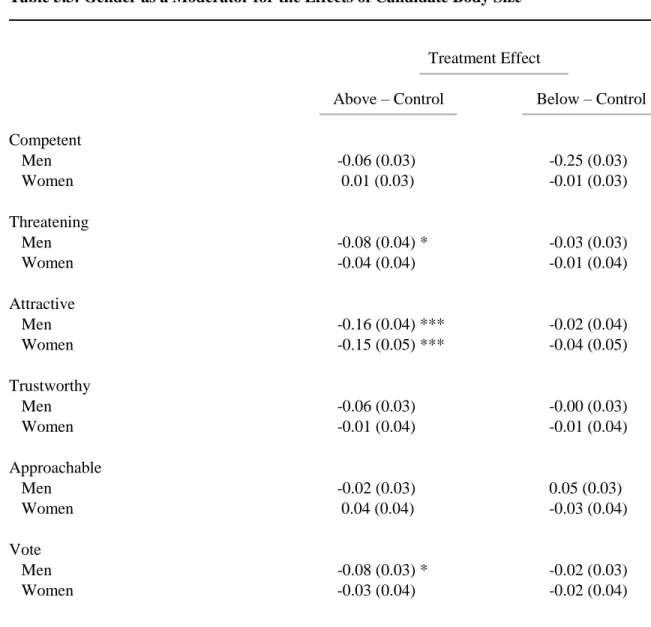
Table 5.3: Gender as a Moderator for the Effects of Candidate Body Size
Treatment Effect
Above – Control Below – Control
Competent
Men -0.06 (0.03) -0.25 (0.03)
Women 0.01 (0.03) -0.01 (0.03)
Threatening
Men -0.08 (0.04) * -0.03 (0.03)
Women -0.04 (0.04) -0.01 (0.04)
Attractive
Men -0.16 (0.04) *** -0.02 (0.04)
Women -0.15 (0.05) *** -0.04 (0.05)
Trustworthy
Men -0.06 (0.03) -0.00 (0.03)
Women -0.01 (0.04) -0.01 (0.04)
Approachable
Men -0.02 (0.03) 0.05 (0.03)
Women 0.04 (0.04) -0.03 (0.04)
Vote
Men -0.08 (0.03) * -0.02 (0.03)
Women -0.03 (0.04) -0.02 (0.04)
Note: N=429, *p<0.05, **p<0.01, ***p<0.001, standard error is reported in parenthesis next to the treatment effect, 239 respondents are male, 190 respondents are female
Table 5.3 reports gender as a moderator for the effects of body size. It is
important to look at gender as a moderator because there are many differences in political
behavior based on gender. For example, men tend to be more conservative than women.
Additionally, the study conducted by Chiao, Bowman, and Gill, and discussed in chapter
between men and women (2008). The table indicates that the male respondents in this
survey perceived the above average sized candidate as being less threatening than the
control. This is not consistent with my hypothesis that the above and below average
candidates would be judged less favorably than the average sized candidate on all
judgments. However, as mentioned previously, this could be because of the stereotype
that those who are larger and less attractive are friendlier. Additionally. Both men and
women in this survey found the above average sized candidate less attractive than the
control. This is consistent with the idea that people who are larger are generally
considered unattractive. Lastly, men in this survey were less likely to vote for the above
average sized candidate, which is consistent with them finding the above average sized
candidate less attractive than the control. As my review of previous research prior to this
data collection found, members of the electorate are less likely to vote for a candidate that
they find unattractive. The fact that women found the above average candidate less
attractive but were not less likely to vote for the above average candidate is also
consistent with the research discussed in chapter one. Chiao, Bowman, and Gill discussed
in chapter one found men prefer a more attractive candidate while women prefer a more
approachable candidate (2008). The fact that the men found the above average candidate
less threatening and were also less likely to vote for him does not align with the results of
Mattes’ study. As discussed previously, he found that members of the electorate were less
likely to vote for a candidate that they found to be threatening (Mattes 2010). However, it
appears that my male participants valued attractiveness over how threatening a candidate
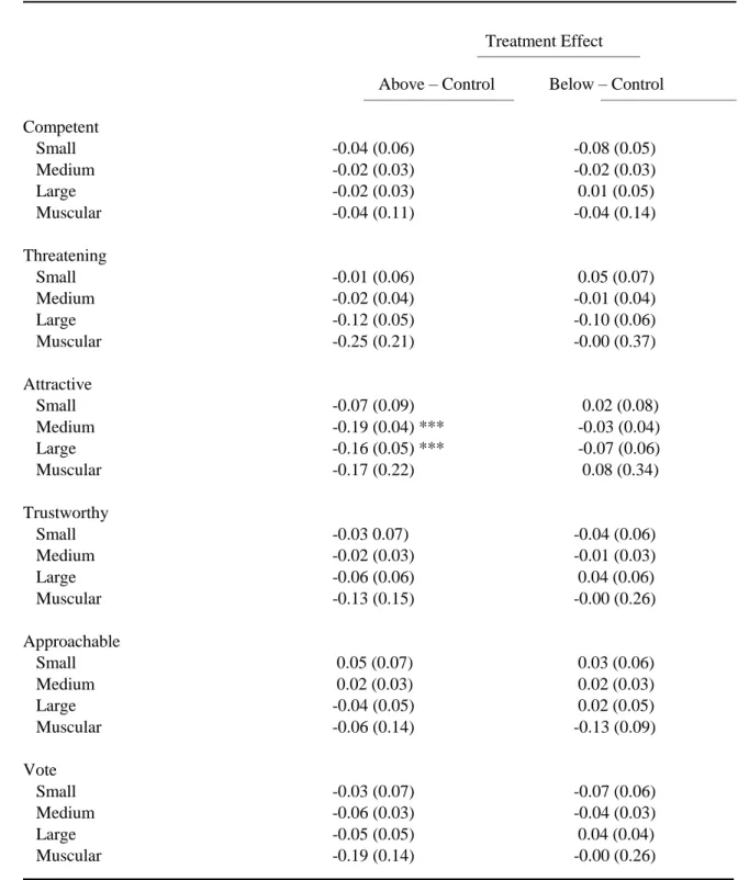
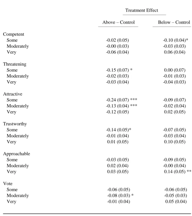
Table 5.4: Perceived Body Size as a Moderator for the Effects of Candidate Body Size
Treatment Effect
Above – Control Below – Control
Competent
Small -0.04 (0.06) -0.08 (0.05)
Medium -0.02 (0.03) -0.02 (0.03)
Large -0.02 (0.03) 0.01 (0.05)
Muscular -0.04 (0.11) -0.04 (0.14)
Threatening
Small -0.01 (0.06) 0.05 (0.07)
Medium -0.02 (0.04) -0.01 (0.04)
Large -0.12 (0.05) -0.10 (0.06)
Muscular -0.25 (0.21) -0.00 (0.37)
Attractive
Small -0.07 (0.09) 0.02 (0.08)
Medium -0.19 (0.04) *** -0.03 (0.04)
Large -0.16 (0.05) *** -0.07 (0.06)
Muscular -0.17 (0.22) 0.08 (0.34)
Trustworthy
Small -0.03 0.07) -0.04 (0.06)
Medium -0.02 (0.03) -0.01 (0.03)
Large -0.06 (0.06) 0.04 (0.06)
Muscular -0.13 (0.15) -0.00 (0.26)
Approachable
Small 0.05 (0.07) 0.03 (0.06)
Medium 0.02 (0.03) 0.02 (0.03)
Large -0.04 (0.05) 0.02 (0.05)
Muscular -0.06 (0.14) -0.13 (0.09)
Vote
Small -0.03 (0.07) -0.07 (0.06)
Medium -0.06 (0.03) -0.04 (0.03)
Large -0.05 (0.05) 0.04 (0.04)
Muscular -0.19 (0.14) -0.00 (0.26)
Next, I report how treatment effects depend on respondents’ description of their
own body type. The purpose of this analysis is to see if how one perceived their own
body size has an effect on how they judge candidates of varying body sizes. Table 5.4
features perceived body size as a moderator for the effects of candidate body size, and
indicates that those who saw themselves as having medium or large body size found the
above average candidate less attractive than the control. There are not enough significant
results here to say that the results are consistent with the idea that, if my hypothesis
failed, it would be because people are voting for a candidate with a body size that
resembles their own. However, the fact that those who saw themselves as large judging
the larger candidate as unattractive serves to contradicts that idea. This could possibly be
because society’s beauty standards seem to be applied to everyone regardless of their
own appearance. Society’s beauty standards are seen as a goal for those who do not
already meet them, and that causes them to judge others accordingly.
These body sizes shown in table 5.3 indicate how the respondents see themselves.
This can be a limitation because a respondent’s perception of their body size is subject to
inaccuracy. The respondents could see themselves as being smaller or larger than they
actually are, or purposely misreport in an attempt to make a good impression. Even so,
perceived body size as a moderator for the effects of candidate’s body size was included
in the calculations because BMI is not always reliable either. The biggest limitation to
BMI is that it fails to account for muscle mass and how one carries their weight. For
example, if one has a lot of muscle mass, or carries their weight in a location on their
body that is not as visible, then they would not look overweight despite their BMI
effects of candidate body size to combat the problems discussed previously regarding
self-reporting. Both perceived body size and actual BMI have their pros and cons
regarding accuracy. Reporting both allows for contrasts between their effects, which is
the best way to overcome their limitations. Additionally, my idea that my hypothesis
would only fail if descriptive factors determined the judgments of the participants relied
on perceived body size. I believed that the perceived body size would matter more than
BMI when determining how closely one relates to a candidate regarding body size
because how people see themselves tends to have the greatest impact on their mental