BRUSH-LIKE POLYMERS: NEW DESIGN PLATFORMS FOR SOFT, DRY MATERIALS WITH UNIQUE PROPERTY RELATIONS
William Francis McKemie Daniel Jr.
A dissertation submitted to the faculty at the University of North Carolina at Chapel Hill in partial fulfillment of the requirements for the degree of Doctor of Philosophy in Chemistry in the
University of North Carolina at Chapel Hill.
Chapel Hill 2017
© 2017
ABSTRACT
William Francis McKemie Daniel Jr.: Brush-Like Polymers: New Design Platforms for Soft, Dry Materials with Unique Property Relations
(Under the direction of Sergei S. Sheiko)
conditions. A solvent-free system also has the potential to be homogeneous which replaces the large energetic interactions with comparatively small architectural interaction parameters.
If a solvent-free alternative to liquid- filled gels is to be created, we must first consider the fundamental barrier to softer elastomers, i.e. entanglements - intrinsic topological restrains which define a lower limit of modulus (~105 Pa). These entanglements are determined by chemistr y specific parameters (repeat unit volume and Kuhn segment size) in the polymer liquid (melt) prior to crosslinking. Previous solvent free replacements for gels include elastomers end-linked in semidilute conditions. These materials are generated through crosslinking telechelic polymer chains in semidilute solutions at the onset of chain overlap. At such low polymer concentratio ns entanglements are greatly diluted and once the resulting gel is dried it creates a supersoft and super-elastic network. Although such methods have successfully generated materials with moduli below the 105 Pa limit and high extensibilities (~1000%) they present their own limitations. Firstly, the semidilute crosslinking methods uses an impractically large volume of solvent which is unattractive in industry. Second, producing and crosslinking large monodisperse telechelic chains is a nontrivial process leading to large uncertainties in the final network architecture and properties . Specifically, telechelics have a distribution of end-to-end distances and in semidilute solutio ns with extremely low fraction of chain ends the crosslink reaction is diffusion limited, very slow, and imprecise. In order to achieve a superior solvent-free platform, we propose alteration of mechanical properties through the architectural disentanglement of brush-like polymer structures.
created from long strands with regularly grafted side chains creating three characteristic length scales which may be independently manipulated. In collaboration with M. Rubinstein, we have utilized bottlebrush polymer architectures (a densely grafted brush-like polymer) to experimenta l ly verify theoretical predictions of disentangled bottlebrush melts. By attaching well-defined side chains onto long polymer backbones, individual polymer strands are separated in space (similar to dilution with solvent) accompanied by a comparatively small increase in the rigidity of the strands. The end result is an architectural disentangled melt with an entanglement plateau modulus as much as three orders of magnitude lower than typical linear polymers and a broadly expanded potential for extensibility once crosslinked.
modulus combined with faster onset of strain hardening which is unseen in single component linear polymer systems.
Transitioning from chemically to physically crosslinked elastomer allows us to create supersoft materials which can be molded into complex shapes and recycled for numerous uses. To facilitate such materials we have generated ABA type triblock copolymers with bottlebrush middle blocks and crystallizable linear A blocks. We have shown the potential for these systems to spontaneously microphase separate into well-defined, super-soft polymer networks which can be easily melted and reformed. The cross-link density was effectively controlled by the DP of the side chains with respect to the DP of the linear tails. Shorter side chains allowed for crystallization of the linear tails of neighboring bottlebrushes forming a soft network without forming a continuo us crystalline phase. However, steric repulsion between longer side chains hindered phase separation and crystallization, thus preventing network formation altogether. Initial stress-strain analysis of these networks display even higher values of 𝛽 (2 to 4 times higher despite possessing longer network strand lengths than those employed by our chemically crosslinked networks). The steric repulsion between the micro phase-separated domains created high pre-extension of the bottlebrush backbones leading to a combination of supersoft modulus with strong strain hardening. Such properties are rarely seen outside of biological tissues and points to ABA type polymers as a forerunner in future research on the topic of mimicking tissue mechanical response.
ACKNOWLEDGEMENTS
TABLE OF CONTENTS
LIST OF TABLES...xiii
LIST OF FIGURES ... xiv
LIST OF ABBREVIATIONS AND SYMBO LS ... xvi
CHAPTER 1: ENTANGLEMENT AND THE BOTTLEBRUSH ARCHITECTURE……..…… .. 1
1.1 The need for soft materials...1
1.2 Linear polymer entanglement ...2
1.3 The bottlebrush architecture...5
1.4 Bottlebrush scaling predictions ...8
1.5 Synthesis of materials ...14
1.6 Molecular characterization...14
1.7 Rheology and mechanical analysis ...20
1.8 Preliminary elastomers...28
1.9 Conclusion and outlook ...31
CHAPTER 2: CHARACTERISATION OF BOTTLEBRUSH ARCHETECTURES...….….….32
2.1 Introduction and objectives ...32
2.2 Synthesis and initial characterization...33
2.3 NMR and GPC analysis ...35
2.4 LB-AFM analysis and results. ...37
2.5 Conclusion and outlook ...46
CHAPTER 3: PROPERTIES OF BOTTLEBRUSH ELASTOMERS...………. ………..48
3.3 Characterization ...51
3.3.1 PDMS Conversion ...51
3.3.2 Mechanical analysis ...51
3.4 Results and discussion ...52
3.5 Conclusion and outlook ...57
CHAPTER 4: PHYSICAL NETWORKS AND GUIDED CRYSTALLIZATION……...58
4.1 Introduction and objectives ...58
4.2 Experimental section...62
4.2.1 Synthesis ...62
4.2.2 Size Exclusion Chromatography and Proton Nuclear Magnetic Resonance ...62
4.2.3 Langmuir-Blodgett Deposition Atomic-Force Microscopy (LB-AFM)...64
4.2.4 Differential Scanning Calorimetry (DSC) ...65
4.2.5 Small/wide angle x-ray scattering ...65
4.2.6 Shear Rheology...65
4.3 Results and discussion ...66
4.4 Conclusion and outlook ...80
CHAPTER 5: GRAFTING DENSITY AND NEW PROPERTY TRENDS………...……….82
5.1 Introduction and objectives ...82
5.2 Experimental section...84
5.2.1 Synthesis ...84
5.2.2 AFM...86
5.2.3 NMR ...87
5.2.4 Stress-strain curves ...87
5.3 Results ...87
5.3.1 Library of polymers and mechanical testing ...87
5.3.2 New mechanical relations ...89
5.4 Conclusion and outlook ...92
LIST OF TABLES
Table 1.1: Initial characterization of materials.………..…16
Table 1.2: LB-AFM analysis of the dimension of PnBA bottlebrushes………...19
Table 1.3: Final molecular characterization………....20
Table 1.4: WLF parameters………..….….…21
Table 2.1: GPC characterization of monomodal and bimodal bottlebrush series………...….3 6 Table 2.2: Results of LB-AFM analyses of monomodal and bimodal bottlebrush series……...….4 0 Table 2.3: The results of AFM and LB analyses for monomodal and bimodal bottlebrushes……..4 2 Table 3.1: Structural parameters and mechanical properties of bottlebrush samples……….…...5 3 Table 4.1: Experimental conditions and molecular parameters for the synthesis of P(HEMA-TMS)……….………..63
Table 4.2: Experimental conditions and molecular parameters for the synthesis of ABA triblock macroinitiator……..……….……….63
Table 4.3: Formulations used for the synthesis of ABA triblock brush………...64
Table 4.4: Structural parameters and LB-AFM size analysis of Triblock bottlebrush polymers….6 8 Table 4.5: Thermal parameters of the bottlebrush samples from DSC and apparent shear moduli……….…………74
Table 5.1: Molecular characterization of PDMS bottlebrushes (𝑛𝑠𝑐 = 14)………...….86
LIST OF FIGURES
Figure 1.1: Transitioning from polymer molecules to mesoscopic filaments………...…6
Figure 1.2: Diagrams of states of brush-like polymers………...…..9
Figure 1.3: Different entanglement modulus regimes of comb-like polymers………...….12
Figure 1.4: GPC traces………...15
Figure 1.5: LB isotherms of surface pressure versus monomer area of linear and bottlebrush BA samples……….….………...16
Figure 1.6: AFM of Bottlebrush samples………....18
Figure 1.7: Overlay of GPC traces……….19
Figure 1.8: Rheological master curve of storage modulus (𝐺′), loss modulus (𝐺′′) and the tangent delta (tan(δ)) as a function of angular frequency……….22
Figure 1.9: Phase angle (δ) vs. complex modulus (𝐺∗)………...……22
Figure 1.10: Comparison of methods………...24
Figure 1.11: Analysis of dynamic mechanical master curves and universal behavior……….2 6 Figure 1.12: Super-soft and super-extendable elastomers……….…….30
Figure 2.1: Initial GPC………..….34
Figure 2.2: GPC of bimodal species………...35
Figure 2.3: AFM of LB monolayers………38
Figure 2.4: AFM of LB monolayers and spin cast bimodal materials……….4 0 Figure 2.5: LB technique………... 43
Figure 2.6: Derivation of dispersity from 2D data……….….46
Figure 3.1: Mechancial response of dense bottlebrush elastomers………...5 5 Figure 3.2: Elastic response………..………..56
Figure 4.2: AFM of 2D crystallized bottlebrush copolymers………..70
Figure 4.3: Width analysis……….….71
Figure 4.4: DSC of bottlebrush copolymer samples……….…..73
Figure 4.5: X-ray………....75
Figure 4.6: Rheological characterization of select bottlebrush copolymers……….…...76
Figure 4.7: Supersoft shape memory………..79
Figure 5.1: Breaking the “Golden Rule” to empower novel mechanical relations………...……...84
Figure 5.2: AFM of bottlebrushes..…………...………..85
Figure 5.3: Synthesis of bottlebrush and comb elastomers………...…..86
Figure 5.4: Tensile curves………...88
LIST OF ABBREVIATIONS AND SYMBOLS
〈R2〉 Mean square end-to-end
a Root mean square end-to-end distance of an entanglement
A0 Area per BA monomer on a Langmuir trough
Abr Area occupied a bottlebrush macromolecule in AFM micrographs
AFM Atomic force microscopy
ATRP Atom transfer radical polymerization
b Kuhn length of chemical monomer
BA Butyl acrylate
bk General Kuhn length
CDCl3 Chloroform
D Chemical monomer diameter
Ð Dispersity
DA Docosyl acrylate
DB Dense bottlebrush
DC Dense comb
DP Degree of polymerization
DSC Differential scanning calorimetry
E Young’s modulus
EMI Electro mechanical instability
G Shear modulus
G’ Storage modulus
G” Loss modulus
G0 Apparent modulus
Ge Shear entanglement modulus
Ge,lin Shear entanglement modulus of a linear polymer
GPC Gel permeation chromatography
HEMA-TMS Trimetylsiloxy)ethyl methacrylate
Ieff Initiation efficiency
K-N Kavassalis-Noolandi
L Contour length of a bottlebrush in an AFM micrograph
l0 Chemical monomer length
LB Loose bottlebrush
LB-AFM Langmuir Blodgett deposition-Atomic force microscopy
LC Loose comb
Le Length of an entanglement
Ln Number average L
lp Persistence length
Lw Weight average L
m mass
m0 Molecular weight of a monomer
Me Entanglement molecular weight
MMA Methyl methacrylate
Mn Number average molecular weight
Mw Weight average molecular weight
n General degree of polymerization
N Number of moles of gas
Nav Avogadro’s number
nbb Degree of polymerization of the backbone ne Degree of polymerization of an entanglement
ne,bb Backbone degree of polymerization of an entanglement ng Number of sidechains per backbone monomer
ng* Crossover ng from combs to bottlebrushes
ng** Crossover ng from loose bottlebrushes to dense bottlebrushes
nm Moles of gas per unit volume
NMR Nuclear magnetic resonance
ns Brush-like stand degree of polymerization nsc Degree of polymerization of a side chain nx Network strand degree of polymerization
ODA Octadecyl acrylate
P Pressure
PAM polyacrylamide
PDMS poly(dimethylsiloxane)
Pe Number of chain segments in an entanglement volume
PnBA poly(n-butyl acrylate)
Psc Number of chain segments in a side chain volume
R Root mean square end-to-end distance
R0 Root mean square end-to-end distance of an ideal flexible chain Rg Root mean square end-to-end distance of a chain segment
between to side chains
Rmax Contour length of a polymer chain
Rsc Root mean square end-to-end distance of a side chain
rT Transfer ration
T Absolute temperature
THF Tetrahydrofuran
Tr Reference absolute temperature
v Mole density
V Volume
v0 Volume of chemical monomer
Ve Physical volume of an entanglement
VGP van Gurp Palmen method
Vp,e Pervaded volume of an entanglement
W Bottlebrush width
WLF Williams–Landel–Ferry
Z Number of molecules per unit are in an AFM micrograph
ΔH Heat of transition from DSC
λ Extension ratio
ρ Mass density
σtrue True stress
τe Entanglement time
CHAPTER 1: ENTANGLEMENT AND THE BOTTLEBRUSH ARCHITECTURE.1
1.1 The need for soft materials
Elastomers are essential soft engineering materials which exhibit relatively low modulus (105-107 Pa) and high extensibility up to 1000%.1 Much of the early focus in elastomer research was based around enhancing mechanical properties i.e. making them stiffer and tougher.2-11 Less attention has been paid to reducing elastomer modulus. However, much softer (10-104 Pa) materials are needed for a number of vital applications. Reconstructive surgery implants require moduli tuned to match the surrounding tissues (as low as 10 Pa) to avoid two universal issues: mechanical irritation and the immune response’s use of mechanical sensing to identify foreign surfaces.12-15 Immature cells differentiate into functional versions based on mechanical cues from the environment. Because of this synthetic materials scaffolds for tissue growth and cell differentiation require a wide variety of attainable moduli in order to design functional biologica l samples.16 - 22 Much like the immune and cell differentiation responses many dangerous microorganisms alter their behavior based on mechanical cues. Specifically on hard surfaces such organisms will switch from vulnerable isolated mobile behaviors to swarming behaviors (a key event in surface fouling and drug resistance in bacterial infection). This makes control of soft mechanical properties key to next generation and antibacterial and antifouling surfaces.23-26 Other
1 Much of this chapter previously appeared in Nature Materials, The original citation follows
important potential applications are found in robotics, membranes, energy storage, and biomedicine.27-52
In traditional elastomeric materials the lower limit of stiffness ca.105 Pa is dictated by chain entanglements that are inherent to polymer melts and, therefore, largely independent of the chemical degree of crosslinking.53-56 In order to achieve moduli lower than 105 Pa a liquid fraction is normally added creating a polymer gel. However, along with many positive features,57-60 the gelation strategy brings about serious limitations due to polymeric gel fragility61 and inherent l y heterogeneous structures.62 Swollen gels may also suffer from environmental instability in the form of phase separations, solvent evaporation, and loss of solvent during deformation.63 Last but not least, the addition of solvent decreases acoustic contrast of materials (particularly, hydrogels), which adversely effects ultrasound imaging of polymeric implants in a human body composed of
ca. 60% water.64-67 Because of the limitations native to gel materials a new class of material needed to be developed which combined the softness of gels with the stability and robustness of elastomers. The first step in the process is to understand the most fundamental mechanica l limitation of soft and dry elastomers, the entanglement.
1.2 Linear polymer entanglement
expressed in simple and familiar terms. Just as ideal gas pressure (𝑃 ≅ 𝑛𝑚𝑅𝑇) is governed by the number of moles of gas per unit volume (𝑛𝑚 = 𝑁 𝑉⁄ ), the modulus of a polymer melt (𝐺𝑒 ≅ 𝜈𝑅𝑇) is governed by mole density of mechanically active strands 𝜈 = 𝜌 𝑀⁄ 𝑒, where – mass density, R
– universal gas constant, T – absolute temperature, and 𝑀𝑒 – molar mass of an entanglement strand. When crosslinked the elastomer traps the entanglements which then behave as additiona l topological crosslinks.68,69 Trapped entanglements impose a preordained lower limit for the elastic modulus, 𝐺 > 𝐺𝑒 ≅ 𝜌𝑅𝑇 𝑀⁄ 𝑒, where 𝐺 – modulus of the crosslinked network. Melts of typical linear polymers possess 𝑀𝑒 ≅ 103− 104 𝑔/𝑚𝑜𝑙, creating an intrinsic entanglement modulus 𝐺𝑒 ≅ 105− 106 𝑃𝑎.54,55 This leads to the question of how to control 𝑀
𝑒.
𝑎3 ≈ (𝑙
0𝑏𝑛𝑒)3/2. The ratio of these two volumes gives the number of chains which exist in the
pervaded volume of a single chains 𝑃𝑒≈ (𝑙0𝑏𝑛𝑒)3/2 𝑣 0𝑛𝑒
⁄ . We can then calculate DP of an entanglement as Equation 1.1.
𝑛𝑒 = 𝑃𝑒2 𝑣02
𝑏3𝑙 𝑜3
1.1
Based on the work from Kavassalis and Noolandi which theorized 𝑃𝑒to be fairly constant between differing chemistries, numerous empirical measurements have found 𝑃𝑒 ≈ 20 for a great many polymers.70 Taking Equation 1.1 we can simplify the expression and solve for 𝑀
𝑒
𝑀𝑒 ≅ 𝑚0𝑃𝑒2 𝑣02
𝑏3𝑙 𝑜3
≅ 𝑃𝑒2𝜌𝑁 𝑎𝑣
𝑣03
𝑏3𝑙 𝑜3
~𝐷6
𝑏3 1.2
where 𝑚0 = 𝜌𝑁𝑎𝑣𝑣𝑜 is the molar mass of the chemical monomer, and 𝐷 ≈ √𝑣0⁄𝑙𝑜 is the approximant diameter of the monomer. As can be seen Equation 1.2 reduces the entire understanding of 𝑀𝑒 and therefore 𝐺𝑒 down some chemical constants and the interplay between the stiffness of a polymer chain (𝑏) and its thickness (𝐷). For traditional materials this interplay is well defined by the chemistry of the polymer chains and results in the traditional limit for polymer melt modulus. In order to create soft materials with moduli below the 105 Pa a new method for increasing the relative thickness of a polymer chain without significantly increasing its stiffness needs to be developed.
1.3 The bottlebrush architecture
of mesoscopic cylindrical filaments. This simple procedure creates two beneficial outcomes: Increasing (i) length (𝐿𝑒) and (ii) diameter (𝐷) of the entanglement strand, leading to an increase of 𝑀𝑒~𝐿𝑒𝐷2 and, hence, decrease of the entanglement plateau modulus as 𝐺
𝑒~ 1 𝑀⁄ 𝑒. However,
this naïve approach does not take into account the fact that conventional solid filaments stiffen as the diameter increases leading to higher entanglement densities (Figure 1.1b). The persistent length of solid filaments is shown, both theoretically71 and experimentally,72 to raise dramatically with their diameter as 𝑙𝑝~𝐷4 (Figure 1.1d) note that 𝑙
𝑝~𝑏𝑘 were 𝑏𝑘 is a general term for the Kuhn
Figure 1.1: Transitioning from polymer molecules to mesoscopic filaments. a) A thought experiment: Affine expansion of a melt of linear chains results in reduction of entangle me nt density (increase of 𝐿𝑒 - length of entanglement strand) and an increase of molecule’s diameter (D). b) The diameter increase causes significant enhancement of rigidity in solid-like filame nts, which generally promotes overlapping with neighbors, increasing the entanglement density. c) A melt of liquid- like flexible filaments displays lower entanglement density than a melt of conventional linear polymers. One of the cylinders (green) displays its interior brush-like structure explored in this study. d) In dilute solution, solid-like filaments display a strong increase of the persistence length with the linear density 𝑀𝐿= 𝑚 𝐿⁄ ~𝐷2 as 𝑙𝑝~𝑀𝐿2~𝐷4 , where m and L and mass and contour length of a filament, respectively, while solvent removal causes additiona l stiffening and ordering of solid filaments.72 In contrast, bottlebrushes remain liquid and their persistence length in a melt state exhibits a much weaker increase with diameter as 𝑙𝑝~𝑀𝐿1 2⁄ ~𝑛𝑠𝑐1 2⁄ ~𝐷, where 𝑛
1.4 Bottlebrush scaling predictions
Herein is presented a summarized version of the theoretical predictions concerning the entanglement modulus of brush-like polymer melts as a function of 𝑛𝑔 and 𝑛𝑠𝑐. For a full treatment please see Daniel, W. F. M., et al. Nat. Mater. 2016, 15, 183-189.
Figure 1.2: Diagrams of states of brush-like polymers. The diagram is presented in terms of degree of polymerization of side chains 𝑛𝑠𝑐 and backbone spacer between neighboring side chains 𝑛𝑔 (logarithmic scales). Comb regimes with almost unperturbed Gaussian backbone and side chains: LC – loosely-grafted combs with strongly interpenetrating neighboring combs, DC – dense combs with weak interpenetration. Bottlebrush regimes: LB – loosely-grafted bottlebrushes with almost unperturbed Gaussian side chains and partially stretched backbone on length scale of side chains, DB – dense bottlebrushes with extended side chains and stretched backbone on length scale of side chains. Dashed lines at 𝑏/𝑙 correspond to boundaries of stiff side chains (vertical) for 𝑛𝑠𝑐 < 𝑏/𝑙, and stiff spacer (horizontal) for 𝑛𝑔 < 𝑏/𝑙. Backbone is almost fully stretched up to length scale of side chain size below the blue horizontal line 𝑛𝑔 ≅ 𝑛𝑔∗∗ ≅ 𝑠.
polymer chain statistics with end-to-end distances 𝑅 = √𝑛𝑏𝑏𝑙0𝑏𝑘,𝐿𝐶 where 𝑏𝑘,𝐿𝐶 = 𝑏 of the specific chemistry used. At the limit of 𝑛𝑔 ≫ 𝑛𝑠𝑐 the contribution of sidechains the total chain volume is negligible and the effective monomer volume is still 𝑣0 ≈ 𝐷2𝑙0. Solving Equation 1.2 reveals
𝑀𝑒,𝐿𝐶 ≈ 𝑀𝑒,𝑙𝑖𝑛 1.3
𝐺𝑒,𝐿𝐶 ≅ 𝜌𝑅𝑇
𝑀𝑒 ≅ 𝐺𝑒,𝑙𝑖𝑛 1.4
Where 𝑀𝑒,𝑙𝑖𝑛 and 𝐺𝑒,𝑙𝑖𝑛 are the entanglement mass and entanglement modulus of the linear polymer chemistry. This results in the flat red domain seen in Figure 1.3a,b. However, as 𝑛𝑔decreases the distance between sidechains 𝑅𝑔 ≤ 𝑅𝑠𝑐 and the sidechains begin to intrude into each other pervaded volumes. This means the average number of other chains segments within a chains pervaded volume (𝑃𝑠𝑐 ≅ 𝑅𝑠𝑐3 (𝑛
𝑠𝑐𝑣0)
⁄ ≅ 𝑛𝑠𝑐1 2⁄ (𝑏𝑙
0)3 2⁄ ⁄𝑣0) is partially occupied buy side
chains from the same polymer backbone. Since 𝑃𝑠𝑐 like 𝑃𝑒 is a constant there are only two options: (1) the chains begin to stretch out thus increasing either 𝑅𝑠𝑐 of 𝑅𝑔 to make more room, or (2) neighboring polymer combs must separate in space leading to fewer interactions between side chains from different combs and an increased effective polymer diameter. Since the stretching of chains carries a heavy entropic penalty55 the combs begin to separate in space diluting their backbones just as if we had added solvent to the system. Because of this the comb maintain their unperturbed chain conformation statistics and 𝑏𝑘,𝐷𝐶 = 𝑏 leading to the expression.
𝑀𝑒,𝐷𝐶~ 𝐷𝐷𝐶6 𝑏𝑘,𝐷𝐶3~
𝑣03
𝑙𝑜3𝑏3(
𝑛𝑠𝑐 𝑛𝑔 + 1)
3
𝐺𝑒,𝐷𝐶 ≅ 𝜌𝑅𝑇 𝑀𝑒 ~ (
𝑛𝑠𝑐 𝑛𝑔 + 1)
−3
1.6
where (𝑛𝑠𝑐⁄𝑛𝑔+ 1)3is the effective contribution of the sidechains towards the molecula r diameter. This trend results is a sharp change in modulus seen as the red line with slope proportional to (𝑛𝑠𝑐⁄ )𝑛𝑔 3 in Figure 1.3a,b.
As the density of sidechains along the backbone grows, the pervaded volume as a single side chain becomes increasingly filled with sidechains belonging to the same backbone. This process continues until there is no longer space for neighboring side chains. A section of a backbone passing through the volume 𝑅𝑠𝑐3 contains on average 𝑛𝑠𝑐 monomers because its conformations are similar to the conformations of side chains. Therefore, 𝑛𝑠𝑐⁄𝑛𝑔 side chains belonging to the same comb molecule and connected to each other through the backbone section containing 𝑛𝑠𝑐 monomers reside within the volume 𝑅𝑠𝑐3. The number of such groups (branched sections) belonging to different comb molecules overlapping with each other within the volume 𝑅𝑠𝑐3 is
𝑍 =𝑃𝑠𝑐𝑛𝑔 𝑛𝑠𝑐 ≅
(𝑏𝑙0)3/2
𝑣𝑜 𝑛𝑔 𝑛𝑠𝑐1 2⁄ ≅
𝑛𝑔
𝑛𝑔∗ ≥ 1 𝑓𝑜𝑟 𝑛𝑔∗ < 𝑛𝑔 < 𝑛𝑠𝑐 (1.7)
Figure 1.3: Different entanglement modulus regimes of comb-like polymers. (Equations 1.4 1.6, 1.9, 1.11) Presented as a function of a) degree of polymerization (DP) of the spacer between neighboring side chains (𝑛𝑔at constant 𝑛𝑠𝑐) and b) side chain DP (𝑛𝑠𝑐at constant 𝑛𝑔).
Loosely-grafted bottlebrush regime (LB). In the LB regime further reduction of 𝑛𝑔 demands deviation from ideal chain statistics. The entropic penalty for stretching all of the sidechains is considerably larger than the penalty of stretching the backbone. In this regime further addition of side chains results in two counteracting phenomenon. First, adding side chains increases the mass of the polymer strands. Second, it stretches the backbone resulting in larger effective 𝑏𝑘 and there for shorter distances between entanglements as shown in Equation 1.1 and 1.2. Because of this the entanglement mass and modulus remain approximately constant while the backbone stretches out leading to the flat green line shown in Figure 1.3a. On the other hand as the sidechain size increases the crossover condition (𝑛𝑔∗~𝑛
𝑠𝑐1 2⁄ ) pushes the loose bottlebrush further
in the regime. The backbone is stretches increasing the chain stiffness as 𝑏𝑘,𝐿𝐵~𝑛𝑠𝑐1/2 while the
chains diameter continues to grow with the ideal sidechains size 𝑅𝑠𝑐~𝑛𝑠𝑐1/2. This dual effect results in the expressions
𝑀𝑒,𝐿𝐵~ 𝐷𝐿𝐵6
𝐺𝑒,𝐿𝐵 ≅𝜌𝑅𝑇
𝑀𝑒 ~ 𝑛𝑠𝑐−3/2 1.9
It should be noted that realistically the LB regime is short. For 𝑛𝑠𝑐 = 100 the regime takes place for only one order of magnitude in 𝑛𝑔 and is much shorter for more typical brushes.
Densely-grafted Bottlebrush Regime (DB). The boundary between the LB and DB regimes (𝑛𝑔 < 𝑛𝑔∗∗= 𝑣
𝑜⁄𝑏𝑙02) corresponds to the fully extended backbone state. At this point the
conformation of the backbone cannot stretch any further without encountering enormous energetic penalties.55 At this point the sidechains begin to weakly stretch leading to an increase in both diameter and rigidity of the polymer strand. This regime is short in terms of 𝑛𝑔 (assuming 𝑛𝑔 = 1 is the practical minimum) but can extend in terms of 𝑛𝑠𝑐 until the sides chains approach the entanglement length of the linear chain chemistry. There is a simultaneous growth of 𝑏𝑘 ,𝐷𝐵 and 𝐷𝐷𝐵 as ~(𝑛𝑠𝑐⁄ )𝑛𝑔 1/2 leading to the equations 1.10 and 1.11 which can be seen in as the blue
lines in Figure 1.3a,b.
𝑀𝑒~ 𝐷𝐷𝐵6 𝑏𝑘,𝐷𝐵3~ (
𝑛𝑠𝑐 𝑛𝑔 )
3/2
1.10
𝐺𝑒,𝐷𝐵≅ 𝜌𝑅𝑇 𝑀𝑒 ~ (
𝑛𝑠𝑐 𝑛𝑔)
−3 2⁄
1.11
1.5 Synthesis of materials
Highly grafted brush-like architectures represent the simplest architecture to produce with reliable homogeneity. They also represent the lowest modulus architectures considered in this dissertation. Because of this, bottlebrushes were chosen as the first architecture for fundame nta l study. The PnBA samples were produced by sequential ATRP steps in which long polymer backbone macroinitiators were synthesized from HEMA-TMS followed by replacing the TMS functionalities with reactive bromine sites and sequential ATRP “polymerize-from” growth of side chains. PDMS samples were produced by ATRP “polymerize-through” of mono-functio na l macromonomers and difunctional crosslinkers inside an evacuated cylindrical mold. For full synthetic details please see Daniel, W. F. M., et al. Nat. Mater. 2016, 15, 183-189.
1.6 Molecular characterization
Monomer conversion and GPC. The conversion of BA was determined from 1H NMR spectra recorded in CDCl3 as a solvent using Brüker 300 MHz spectrometer. Molecular weight distributions of the polymers were characterized by gel permeation chromatography (GPC) using Polymer Standards Services (PSS) columns (guard, 105, 103, and 102 Å), with THF eluent at 35 °C, flow rate 1.00 mL/min, and differential refractive index detector (Waters, 2410). The apparent number-average molecular weights (Mn) and molecular weight dispersities (Mw/Mn) were determined with a calibration based on linear poly(methyl methacrylate) (PMMA) standards and diphenyl ether as an internal standard, using
WinGPC 6.0 software from PSS (Figure 1.4). Bottlebrush samples were analyzed by GPC with light scattering detection to measure molecula r weight distribution of cleaved side chains (Figure 1.4). The initiation efficiency of the grafting- fro m reaction was determined as a ratio of the DP values obtained from monomer conversion (NMR) and side-chain cleavage. The average grafting efficiency is about 0.65 (65%) which is close to the grafting density obtained by the LB-AFM
techniques. The backbone DP by GPC of the macroinitiator as 𝑛𝑏𝑏 = 𝑀𝑀𝐼⁄𝑀0 = 2,035 ± 100. The NMR GPC analysis is summarized in table 1.1. However both techniques are less reliable for analysis of branched molecules so additional analysis was conducted using the LB-AFM technique.
Figure 1.4: GPC traces. Linear (gray) MI-TMS and (black) MI-Br, and bottlebrushes (red) BA-3/4, (orange) BA-17, (yellow), BA-23, (pale green), BA-34, (dark green), BA-130, and (blue) BA-112.
104 105 106 107
Table 1.1 Initial characterization of materials
Name Composition nsc,NMR 1 Mn,GPC2
Mw/
Mn2 Mn,SC
3 M
w/Mn,sc3 nsc4 Ie ff5
MI-TMS P(HEMA-TMS)2035 - 326,000 1.29 - - - -
MI-Br PBiBEM2035 - 694,000 1.76 - - - -
BA-6 PBiBEM2035-g
-PnBA3/4 3-4 640,000 1.76 - - - -
BA-17 PBiBEM2035-g
-PnBA10 10 1,540,000 1.19 2,180 1.12 17 59
BA-23 PBiBEM2035-g
-PnBA16 16 1,870,000 1.19 3,000 1.18 23 70
BA-34 PBiBEM2035-g
-PnBA24 24 2,070,000 1.20 4,300 1.30 34 70
BA-130 PBiBEM2035-g
-PnBA48 48 3,380,000 1.13 16,600 1.10 130 40 1Degree of polymerization of side-chains determined from the monomer conversion by 1H NMR, nsc,NMR = ntargeted Mconversion. 2 Determined by THF GPC using PMMA standards. The GPC data are inaccurate due to the large size and branched nature of the macromolecules. 3 Number average molecular weight and PDI of cleaved side chains determined by THF GPC using PSt standards. 4 Degree of the polymerization of side chains determined from the equation: nsc = Mn,sc / MBA, where MBA=128 – molecular weight of n-butyl acrylate 5 Initiation efficiency determined as Ieff = (nsc,NMR / nSC)100%.
LB-AFM. The large spatial dimensions of bottlebrush molecules enable visualization by AFM. Combining this with the Langmuir Blodgett deposition technique was shown in the past to be an accurate analysis technique for bottlebrushes.82 The
samples for atomic force microscopy (AFM) studies were prepared by Langmuir-Blodgett (LB) deposition (Figure 1.5). LB films were transferred onto freshly cleaved mica substrates at a constant surface pressure of 0.5 mN/m and a controlled transfer ratio. Imaging
QNM mode using a multimode AFM (Brüker) with a NanoScope V controller. Silicon probes were used with a resonance frequency of 50-90 Hz and a spring constant of ~0.4 N/m. In-house developed computer software was used to analyze the AFM images. Typically, ensembles of 1000 or more molecules were analyzed to ensure standard deviation of the mean below 10%. The results are summarized in Table 1.2. The number-average contour length (𝐿) were directly extracted from the AFM micrographs of individual macromolecules both in dense and sparse monolayers on a solid substrate (Figure 1.6) as 𝑛𝑏𝑏 = 𝐿 𝑙 = 2,040 ± 60⁄ . All molecular length scales characterized by LB-AFM are disabled in Table 1.2.
From the LB-AFM analysis, we determine the number average mass per unit length of the backbone, which can be directly translated to the side-chain degree of polymerization per monomeric unit of the backbone as
𝑛𝑠𝑐 𝑛𝑔 =
𝑟𝑡𝐴𝑏𝑟 𝑛𝑏𝑏𝐴0 =
𝑟𝑡𝑙0(𝑊 + 𝜋𝑟𝑡𝑊2
4𝐿 )
𝐴0 1.12
agreement with 𝑛𝑏𝑏 = 2040 ± 60 determined by LB-AFM (Table 1.3). The full extension of the bottlebrush backbones is caused by steric repulsion of densely grafted side chains resulting in a backbone tension of the order of 1 nN.83 The product of linear mass density and bottlebrush contour length gives molecular weight distribution (MWD). Figure 1.7 demonstrates correlation between the MWD data obtained by the GPC and LB-AFM techniques. A slight shift towards higher molecular weights seen in the LB-AFM is due to exclusion of small species analysis software. The number-average contour length were directly extracted from the AFM micrograp hs of individual macromolecules both in dense and sparse monolayers on a solid substrate (Figure 1.6) as 𝑛𝑏𝑏 = 𝐿 𝑙 = 2,040 ± 60⁄ . The complete molecular characterization is presented in Table 1.3.
Figure 1.7: Overlay of GPC traces. Bottlebrush samples (red histograms) with LB-AFM molecular weight distribution analysis (black lines). The green lines correspond to molecular weight distribution of the macroinitiators (backbones without side chains).
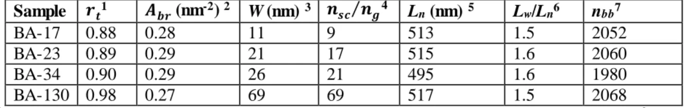
Table 1.2: LB-AFM analysis of the dimension of PnBA bottlebrushes
Sample 𝒓𝒕1 𝑨𝒃𝒓 (nm-2) 2 W (nm) 3 𝒏𝒔𝒄⁄𝒏𝒈4 Ln (nm) 5 Lw/Ln6 n
bb7
BA-17 0.88 0.28 11 9 513 1.5 2052
BA-23 0.89 0.29 21 17 515 1.6 2060
BA-34 0.90 0.29 26 21 495 1.6 1980
BA-130 0.98 0.27 69 69 517 1.5 2068
Table 1.3: Final molecular characterization
Sample M,
1
106 g/mol
𝒏𝒔𝒄2
(cleavage)
𝒏𝒔𝒄⁄𝒏𝒈3
(LB-AFM)
𝒏𝒈4 Ð 5 Ge, Pa6 Me,
7
106 g/mol 𝒏𝒆,𝒃𝒃 8
MI9 0.3310 0 0 NA 1.3 NA NA NA
BA-6 NA11 NA 3 1.75 NA 11432 ± 331 0.2 461±13
BA-17 2.9 17 9 1.96 1.5 2421 ± 75 1.1 784±24
BA-23 4.7 23 14 1.61 1.6 1310 ± 54 2.1 894±37
BA-34 5.8 34 21 1.61 1.6 938 ± 28 2.9 1012±30
BA-130 17.9 130 67 1.89 1.5 178 ± 7 15.2 1728±68
1Number average molar mass determined from mass per unit area and molecular area using the LB-AFM method (except MI).31 2Number average DP of side chains determined by GPC of cleaved side chains. 3Number average DP of side chains multiplied by the grating density 𝑛
𝑔−1 as
measured by LB-AFM (Equation 1.12). 4Grafting density calculated from LB-AFM 𝑛
𝑠𝑐⁄𝑛𝑔 and
cleavage 𝑛𝑠𝑐. 5Dispersity of PnBA bottlebrush contour length, PDI=L
w/Ln, where Lw and Ln are weight and number average contour lengths of the bottlebrush backbones. 6Plateau modulus determined as storage modulus at the frequency of the minimum in tan(δ). Modulus error was calculated by taking the standard error of the mean from multiple measurements of the master curve. 7Molar mass of the entanglement strand calculated as 𝑀
𝑒 = 𝜌𝑅𝑇 𝐺⁄ 𝑒, where 𝜌 =
1.09 𝑔/𝑐𝑚3 – mass density of PnBA. 8Backbone DP of the entanglement strand calculated as 𝑛𝑒,𝑏𝑏 ≅ 𝑀𝑒𝑛𝑏𝑏⁄𝑀, where M - molar mass of bottlebrush and 𝑛𝑏𝑏=2040- average DP of the backbone. 9Macroinitiator (MI) is a precursor for the backbone. 10Number average molecular weight measured by RI-GPC using PMMA standards. 11AFM-based analysis of BA-6 was inaccurate due to closely spaced macromolecules having the shortest side chains.
1.7 Rheology and mechanical analysis
experiments were done with an RSA-G2 DMA from TA instruments using 25mm compression plates at a constant closure rate of 0.01 mm/s at 25°C. Based on the time-temperature superpositio n principle, master curves of modulus versus frequency were constructed using TRIOS software from TA instrument. A series of Williams–Landel–Ferry (WLF) parameters was generated using eq 1.13 for each sample and used to shift the final master curves to 298 K
log(𝛼𝑡) =−𝐶1(𝑇−𝑇𝑟)
𝐶2+(𝑇−𝑇𝑟) 1.13
where 𝛼𝑡 -frequency shift factor for a desired reference temperature, 𝐶1and 𝐶2-empirical fitting constants derived from manual shifts of data at multiple temperatures, 𝑇 and 𝑇𝑟 - sample temperature and desired reference temperature, respectively.84 Table 1.4 summarizes the corresponding WLF parameters.
Three methods were used to analyze the entanglement plateau modulus of the polymer samples. Figure 1.10 shows trends of entanglement moduli versus relative side-chain length. Both methods for assigning entanglement moduli give excellent agreement with theory showing dependence on relative side-chains DP (𝐺𝑒~(𝑛𝑠𝑐⁄𝑛𝑔+ 1)−3/2) as shown in Figure 1.10 below.
For the first method the value of the entanglement modulus is taken as the value of 𝐺′ at the frequency of the minimum in the tangent delta as described in detail by Lomellini85 (Figure 1.8). Entanglement modulus and tangent delta data is represented in Table S4 and the trend in entanglement modulus versus relative sidechains DP is displayed in black in Figure 1.10.
Table 1.4: WLF parameters
sample C1 C2 (K)
BA-6 7.3 129.2
BA-17 3.9 153.9
BA-23 3.5 154.4
BA-34 3.8 161.8
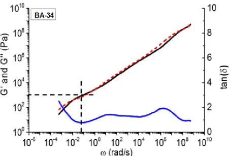
Figure 1.8: Rheological master curve of storage modulus (𝑮′), loss modulus (𝑮′′) and the
tangent delta (tan(δ)) as a function of angular frequency. The vertical and horizontal dashed line mark the minimum of tangent delta and the entanglement modulus, respectively.
For the second method the van Gurp Palmen method assigns the entanglement modulus as the value of the storage modulus at the minimum in phase angle within the entanglement regime of a VGP plot86 (Figure 1.9). The moduli versus relative sidechains size are displayed in red in Figure 1.10.
Figure 1.9: Phase angle (δ) vs. complex modulus (𝑮∗). The entanglement modulus is assigned
For the third method, the value of the storage modulus determined by modeling experimental data with a fitting equation described below. To evaluate the rheological data we model the storage modulus 𝐺′() and loss modulus 𝐺′′ () using the molar mass weight 𝑀𝑒 as a fitting parameter. The storage and loss modulus can be presented as the sine and cosine transform of the time dependent modulus G(t)55,87:
𝐺′(𝜔) = 𝜔 ∫ 𝐺(𝑡) sin(𝜔𝑡) 𝑑𝑡 ∞
0
1.14
𝐺′′(𝜔) = 𝜔 ∫ 𝐺(𝑡) cos(𝜔𝑡) 𝑑𝑡 ∞
0
1.15
A model for G(t) includes two distinct regions of rheological behavior seen in the bottlebrush sample. These are Region 1: power law relaxation with exponent 0.6 representing transition zone of chain of effective Kuhn monomers, where 𝐺1and 𝜏𝑡 are the modulus and relaxation time of the effective Kuhn monomer. Note 𝐺1and 𝜏𝑡serve to shift the date to allow overlap between the power law and experimental data. As their specific values do not have physical meaning in the applicatio n of this theory
𝐺(𝑡)𝑝𝑜𝑤𝑒𝑟 = 𝐺1(𝑡 𝜏1)
−0.6
1.16
and Region 2: entanglement relaxation. For monodisperse melts, as the entanglement relaxatio n can be approximated by a single exponential decay
𝐺(𝑡)𝑅𝑒𝑝𝑡 =𝜌𝑅𝑇 𝑀𝑒 exp
[
− 𝑡
𝜏𝑒 ( 𝑀𝑀
𝑒) 3.4
]
1.17
the molar mass of the brush species. To account for molar mass polydispersity, we use the double reptation model as the square of the integral of the conventional reptation relaxation multiplied by the weight fraction of each respective species over all molar mass species88
𝐺(𝑡)𝑅𝑒𝑝𝑡𝑎𝑡𝑖𝑜𝑛 =𝜌𝑅𝑇
𝑀𝑒 (∫ 𝑤𝑖𝑒 −𝑡
𝜏𝑒(𝑀𝑚𝑖
𝑒) 3.4 ⁄ ∞ 0 ) 2 1.18
where wi and mi are the weight fraction and molar mass of a species. For discrete molar mass distribution data, the final model was described as
𝐺(𝑡) = 𝐺1(𝑡 𝜏1)
−0.6
+𝜌𝑅𝑇
𝑀𝑒 (∑𝑤𝑖𝑒 −𝑡
𝜏𝑒(𝑚𝑀𝑖
𝑒) 3.4 ⁄ 𝑖=𝑘 𝑖=1 ) 2 1.19
where G1/τ1-0.6, Me, and τe are the fitting terms used to fit the model with the experimental data. The entanglement modulus versus the relative side chain DP are displayed in blue in Fig. 1.10. A sample overlay of the fitting and experimental data is shown in Fig. 1.11c.
Figure 1.10: Comparison of methods. Comparison of entanglement modulus analysis methods yields excellent agreement with theoretical trend of 𝐺𝑒~(𝑛𝑠𝑐⁄𝑛𝑔 + 1)−3/2.
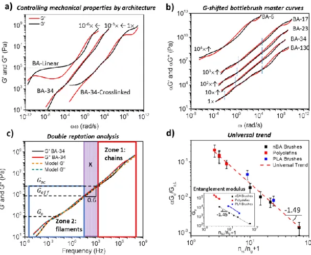
Figure 1.11d displays the dependence of the plateau modulus on 𝑛𝑠𝑐⁄ 𝑛𝑔 + 1 - reciprocal volume fraction of bottlebrush backbones. To enable comparison with similar structures reported previously by other groups, we plot the modulus ratio of bottlebrush and linear polymers multip l ied by a dimensionless parameter 𝛼 = (𝑣 𝑏⁄ 2𝑙)−3 2⁄ accounting for the difference in chemica l composition (Equation 1.11). Remarkably, all data points, including that of (i) our PnBA bottlebrushes, (ii) pLA bottlebrushes studied by Kornfield et al.,80 and (iii) dense polyolefin combs studied by Fetters et al.77 fall on one line with a slope of -1.490.05 in agreement with Equation 1.11. The bottlebrush melt (𝑛𝑠𝑐 = 130) displays modulus on the order of 100 Pa, which is three orders of magnitude lower than the 𝐺𝑒of linear PnBA. This low modulus is ascribed to the significant decrease of the entanglement density in bottlebrush melts composed of thick, flexib le, and weakly-interpenetrating macromolecules. As shown in Table 1.3, both the molar mass of the entanglement strand (𝑀𝑒≅ 105− 107 𝑔/𝑚𝑜𝑙) and the DP of its backbone (𝑛
𝑒,𝑏𝑏 ≅ 500 − 2,000)
are significantly larger than the corresponding values for linear PnBA, 𝑀𝑒 ≅ 2 × 10⁴ 𝑔/𝑚𝑜𝑙 and
Figure 1.11: Analysis of dynamic mechanical master curves and universal behavior. a) Frequency-shifted master curves for the storage (G’) and loss (G”) moduli of PnBA linear and bottlebrush polymer melts, and a randomly cross-linked bottlebrush elastomer of BA-34 at 25C. Linear PnBA displays characteristic entanglement plateau, while BA-34 display power-law relaxation and weak entanglement plateau at significantly lower modulus. The cross-linked sample displays similar power-law relaxation followed by an elastic modulus ~100 times lower than 𝐺𝑒 of linear PnBA. b) Vertically modulus-shifted master curves of five PnBA bottlebrush samples from Table 1.2 c) Overlay of experimental rheological master curves (BA-34 at T=25C) with the double-reptation fit. Two distinct zones (1,2) and a crossover (X) region are observed: (1) relaxation of polymer chains, (2) relaxation of bottlebrush filaments considered as chains of effective monomers, and (X) internal relaxation modes of the effective monomer displaying power-law dependence 𝐺′ ≅ 𝐺′′~𝜔0.6 . d) Log-log plots of the plateau modulus ratio of bottlebrush and linear chain melts (𝐺𝑒⁄𝐺𝑒,𝐿) as a function of the reciprocal backbone volume fraction determined by DP of bottlebrush side chains (𝑛𝑠𝑐) and grafting density (𝑛𝑔−1). The data
Additional analysis of the modulus relaxation spectrum identified two characteristic zones in the master curves (Figure 1.11c). Zone 1 (linear chains) includes high frequency glassy and transition relaxation modes of individual chains common to all polymers displaying close match of both the 𝐺′ curves and 𝐺′′ curves. Zone 1 has a lower bound corresponding to relaxations on the scale of the side chain (solid vertical lines Figure 1.11b) (𝐺𝑠𝑐 ≈ 𝑘𝑏𝑇/𝑛𝑠𝑐𝑣), beyond which side chains motions become correlated through the backbone. At lower frequencies, we observe Zone 2 (bottlebrush filaments), which corresponds to the relaxation of filament strands comprised of effective monomers of size 𝐷 ≅ (𝑛𝑠𝑐𝑙𝑏)1/2 - filament diameter. Zone 2 has an upper bound determined by the size of the effective monomer (𝐺𝑒𝑓𝑓 ≈ 𝑘𝑏𝑇/𝐷3), which indicates the onset of
1.8 Preliminary elastomers
The architectural reduction of entanglement density within bottlebrush melts provides access to a new range of properties for the design of elastomers with unprecedentedly low elastic modulus and high deformability. In order to expand the super-soft concept from melts into solid materials, and to demonstrate the universality of our method as it relates to differing chemical structures, we have synthesized a series of poly(dimethylsiloxane) (PDMS) bottlebrush elastomers (𝑛𝑠𝑐 = 14 and 𝑛𝑔 = 1) with systematically controlled cross-linking densities using ATRP of mono and di-functional macromonomers. For these values of 𝑛𝑠𝑐 and 𝑛𝑔, our scaling analys is predicts the following dimensions of the entanglement strand: 𝑛𝑒,𝑏𝑏 ≅ 2,900 (backbone DP) and 𝑀𝑒≅ 2.9 × 10⁶ 𝑔/𝑚𝑜𝑙 (molar mass). Melts comprised of such PDMS bottlebrushes are expected
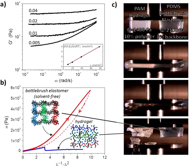
to exhibit an entanglement modulus of 𝐺𝑒 ≅ 800 𝑃𝑎, which (within a numerical prefactor on the order of 1) sets a lower boundary for elastic modulus of PDMS bottlebrush elastomers with 𝑛𝑠𝑐 = 14 and 𝑛𝑔 = 1. In agreement with this prediction, Figure 1.12a shows a consistent modulus decrease down to 520 Pa with decreasing crosslinking density, which is ca. 400 times softer than 𝐺𝑒,𝑙𝑖𝑛 ≅ 200 𝑘𝑃𝑎 measured for linear PDMS melts. Furthermore, the effective dilution of chain
entanglements in bottlebrush melts not only reduces the elastic modulus, but also allows higher deformation of the corresponding elastomers.
stress measurements in Figure 1.12b, bottlebrush elastomers exhibit superior deformability with elastomer-like compression ratio of 𝜆−1 = 𝐿0⁄ ≅ 10 while possessing similar modulus to the 𝐿 gel counterpart (~2,000 Pa). The work of compression at fracture was then measured as 𝑊 ≅ 0.2 𝑀𝐽 𝑚⁄ 3, which is approximately one order of magnitude larger than that of conventional linear
Figure 1.12: Super-soft and super-extendable elastomers. (a) Poly(dimethylsiloxane) (PDMS) bottlebrush elastomer displaying moduli on the order of 100 to 1000 times softer than linear PDMS entanglement modulus as a function of crosslinker/macromonomer fraction as indicated. Inset: The plateau modulus decreases with calculated crosslinking density, where the slope gives 5% crosslinker reactivity and the zero- intercept suggests ca. 10% of dangling strands. (b) True stress was measured during compression of a pDMS bottlebrush elastomer and poly(acrylamide) (PAM) hydrogel possessing similar volume fractions of backbones and polymer chains, respectively. The bottlebrush elastomer exhibit considerably higher fracture energy than gel counterparts, while both materials show a similar modulus of ~2000 Pa. Bottlebrush samples display considerably higher compressibility (compression ratio at break 𝜆−1= 𝐿
0⁄ ≅ 10 for bottlebrushes and 𝜆𝐿 −1 ≅ 3 for
1.9 Conclusion and outlook
CHAPTER 2: CHARACTERISATION OF BOTTLEBRUSH ARCHETECTURES2
2.1 Introduction and objectives
The previous chapter displays the mathematical relations between modulus and brush- like architectural parameters. These relations ultimately rely on the fraction of side chains (𝑛𝑠𝑐⁄𝑛𝑔) thus making accurate characterization of this quantity paramount. For this purpose we turn to the 2D properties of bottlebrushes. Bottlebrush molecules have large molecular dimensions allowing for accurate counts of individual molecules and accurate measurements of 𝑛𝑏𝑏 assuming a fully extended backbone at low values of 𝑛𝑔. In past studies this architectural property has been used to discover a series of interesting properties including flow-enhanced molecular diffusion, 90 epitaxial ordering,91 and conformational transitions92 that triggered flow instability.93 Molecular sensors have been designed to gauge both pressure gradient and friction coefficient at the substrate.92 These studies culminated with the discovery of scission of covalent bonds during adsorption and spreading of branched macromolecules on a substrate.94-96 All of these fascinating properties occur due to the interactions between bottlebrush side chains and 2D substrates, however the rules governing how side chains differentiate themselves into a population which is
2This chapter previously appeared as an article in Macromolecules. The original citation is as follows: Burdyńska, J.; Daniel, W.; Li, Y.; Robertson, B.; Sheiko, S. S.; Matyjaszewski, K.
adsorbed onto a surfaces and a population forced into a cone above the substrate. While the adsorbed side chains chain extend to maximize the area of the substrate covered by the deposited brush, the desorbed side chains form a “cap” sitting on top of the monolayer of the adsorbed side chains.82 The conformation of surface-confined bottlebrushes, including the length, width, and flexibility, or persistence length of the backbone, is largely controlled by the fraction of adsorbed side chains. However, if the side chains exhibit broad polydispersity, the conformation also depends on the length distribution of adsorbed and desorbed side chains. There are two possible adsorption processes. In one case the adsorption process is random and the dispersity of the adsorbed side chains is equal to the overall dispersity. In another case, favoring adsorption of the longest side chains, one should observe a large separation between adsorbed macromolecules and also an increased width of single molecules due to predominate adsorption of the longest side chains. In this chapter we explore the relation between side chain distribution and side chain adsorption as well as use AFM to accurately analysis 𝑛𝑠𝑐⁄𝑛𝑔.
2.2 Synthesis and initial characterization
2.3 NMR and GPC analysis
The conversion of monomers was determined from 1H NMR spectra recorded in CDCl3 using a Brüker 300 MHz spectrometer. Molecular weight distributions of the polymers were characterized by gel permeation chromatography (GPC) using Polymer Standards Services (PSS ) columns (guard, 105, 103, and 102 Å), with THF eluent at 35 °C, flow rate 1.00 mL/min, and differential refractive index (RI) detector (Waters, 2410). The apparent number-average molecular weights (Mn) and molecular weight dispersities (Mw/Mn) were determined with a calibration based on linear poly(methyl methacrylate) (PMMA) standards and diphenyl ether as an internal standard, using WinGPC 6.0 software from PSS (Figure 2.2, Table 2.1). Bottlebrush samples were analyzed by GPC with light scattering detection to measure molecular weight distribution.
The chain-extension to form bottlebrushes 20-80 and 50-50 was confirmed by the shift of GPC traces towards higher molecular weight values, when compared to sample 0-100 (Figure 2.2, blue and red). In all cases GPC signals were monomodal with narrow molecular weight distributions (Ð~1.2) demonstrating the formation of well-defined bottlebrushes (Table 2.1). However, a more detailed analysis of GPC traces of 20-80 and 50-50 showed the appearance of low molecular weight peaks, which was ascribed to the formation of a linear PnBA with yet unknown mechanistic origin. The low molecular weight impurities present in brushes 20-80 and 50-50 was removed via selective precipitation of the bottle brushes from THF solution into methanol at room temperature, providing pure samples of the bimodal bottlebrushes.
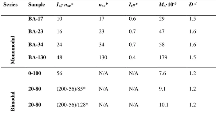
Table 2.1: GPC characterization of monomodal and bimodal bottlebrush series.
Series Sample Ieff nsc a nsc b Ieff c Mn·10-5 Ð d
M
on
om
od
al
BA-17 10 17 0.6 29 1.5
BA-23 16 23 0.7 47 1.6
BA-34 24 34 0.7 58 1.6
BA-130 48 130 0.4 179 1.5
B
im
od
al
0-100 56 N/A N/A 7.6 1.2
20-80 (200-56)/85* N/A N/A 9.1 1.2
20-80 (200-56)/128* N/A N/A 10.1 1.2
a Number average degree of polymerization of side chance calculated from the monomer conversion determined by 1H NMR, using the equation: 𝐼
𝑒𝑓𝑓 𝑛sc = (1 −
𝐴[𝑀]×𝐴[𝐴𝑛𝑖𝑠𝑜𝑙𝑒]0
𝐴[𝑀]0×𝐴[𝐴𝑛𝑖𝑠𝑜𝑙𝑒]) ×
the grafting process d Dispersity of bottlebrush polymers Ð =Mw/Mn determined by THF GPC using PS standards. *Determined from the equation: 𝑛
𝑠𝑐 = 𝑛𝑠ℎ𝑜𝑟𝑡 × 𝑥𝑠ℎ𝑜𝑟𝑡 + 𝑛𝑙𝑜𝑛𝑔 × 𝑥𝑙𝑜𝑛𝑔 ,
where 𝑛𝑠ℎ𝑜𝑟𝑡 and 𝑛𝑙𝑜𝑛𝑔 are degrees of polymerizations corresponding to short and long grafts of bimodal bottlebrushes, and 𝑥𝑠ℎ𝑜𝑟𝑡 and 𝑥𝑙𝑜𝑛𝑔 are their respective mole fractions.
2.4 LB-AFM analysis and results.
The combination of AFM and the LB techniques is a very powerful method for quantitat ive characterization of the geometric dimensions and molecular weight distribution of branched macromolecules. While the LB technique allows for preparation of well-defined monolayers under controlled surface area per monomeric unit (𝐴𝐵𝑅0), AFM provides images of individ ua l bottlebrush molecules within these monolayers (Figure 2.3). By counting the number of molecules per unit area(𝐴𝐵𝑅−1), the number average molecular weight was determined as 𝑀 = 𝑀
0𝑁𝐴𝑣𝐴𝐵𝑅/
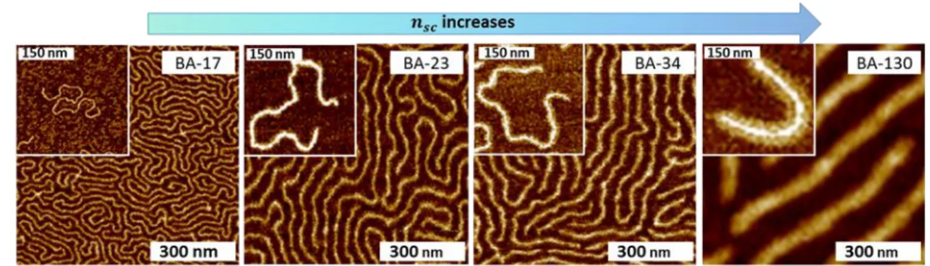
Figure 2.3: AFM of LB monolayers. AFM height images of monomodal bottlebrushes with different degrees of polymerization (𝑛𝑠𝑐) of the side chains. Images were taken from LB trough monolayers transferred onto mica substrates.
Table 2.2: Results of LB-AFM analyses of monomodal and bimodal bottlebrush series
Series Entry W
a / nm La / nm
spin cast LB LB
M
onom
oda
l BA-17 N/A 11±1 513±18
BA-23 N/A 18±1 515±18
BA-34 N/A 26±3 495±25
BA-130 N/A 69±5 517±3
B
im
oda
l
0-100 50±4 51±2 134±2
20-80 short 50±7 78±4 133±3
long 63±4
50-50 short 58±5 98±8 130±2
long 82±4
a Length (L) and width (W) of bottlebrushes obtained from AFM images of LB films or spin casted bottlebrushes on mica substrates.
Figure 2.4: AFM of LB monolayers and spin cast bimodal materials . 22 m2 AFM height micrographs of LB monolayers prepared from bottlebrushes with a) monomodal, 0-100, 𝑛𝑠ℎ𝑜𝑟𝑡=56, and bimodal graft lengths b) 20-80, 𝑛𝑙𝑜𝑛𝑔=200 (80%) and 𝑛𝑠ℎ𝑜𝑟𝑡= 56 (20%), and c) 50-50, 𝑛𝑙𝑜𝑛𝑔=200 (50%) and 𝑛𝑠ℎ𝑜𝑟𝑡= 56 (50%), on a mica surface; Images of single brush molecules prepared by spin-casting methods are shown in circles (the scale bar is 200 nm). Black and red arrows indicate the dense core of the shorter side chains and diffusive hallo of the longer grafts, respectively.
that of linear PnBA (𝐴𝐿,0). The ratio 𝜙𝑚 = 𝐴𝐵𝑅,0⁄𝐴𝐿,0 provides quantitative information about the fraction of adsorbed monomers.Error! Bookmark not defined. In the case of monomodal brushes the 𝐴
𝐵𝑅 ,0