DISCRIMINATIVE REPRESENTATIONS FOR HETEROGENEOUS IMAGES AND MULTIMODAL DATA
Heather D. Couture
A dissertation submitted to the faculty of the University of North Carolina at Chapel Hill in partial fulfillment of the requirements for the degree of Doctor of Philosophy in
the Department of Computer Science.
Chapel Hill 2019
Approved by:
Marc Niethammer
Alex Berg
J.S. Marron
Charles M. Perou
c
2019
ABSTRACT
Heather D. Couture: Discriminative Representations for Heterogeneous Images and Multimodal Data
(Under the direction of Marc Niethammer)
Histology images of tumor tissue are an important diagnostic and prognostic tool for pathol-ogists. Recently developed molecular methods group tumors into subtypes to further guide treatment decisions, but they are not routinely performed on all patients. A lower cost and repeatable method to predict tumor subtypes from histology could bring benefits to more can-cer patients. Further, combining imaging and genomic data types provides a more complete view of the tumor and may improve prognostication and treatment decisions. While molecular and genomic methods capture the state of a small sample of tumor, histological image analysis provides a spatial view and can identify multiple subtypes in a single tumor. This intra-tumor heterogeneity has yet to be fully understood and its quantification may lead to future insights into tumor progression.
ACKNOWLEDGMENTS
First and foremost, I want to express my gratitude to my advisor, Marc Niethammer. He has provided immense guidance, encouragement, and support throughout the last seven years, starting even before I applied to the graduate program at UNC. He made the decision to return to school for a Ph.D. an easy one. He gave me the freedom to explore different research directions and helped refine my writing skills. He challenged me to think about theory and design clear experiments. He accommodated me in working remotely, allowing for work/life balance while raising a family. I appreciate his dedication to both teaching and advising.
I also want to thank the other professors on my committee. Steve Marron provided a continuous source of insightful advice and feedback on my research. I appreciate his focus on model interpretability and eagerly await future contributions from his group in this area. Chuck Perou has been essential in contributing knowledge of breast cancer genomics and guiding this project in a clinically important direction. Steve Pizer provided my first introduction to medical image analysis and has continued to contribute valuable and insightful feedback on my research presentations and this dissertation. Alex Berg provided valuable feedback on my research through his expertise in computer vision and machine learning.
I am also grateful to a number of other collaborators. Melissa Troester provided extensive knowledge in breast cancer research, guidance towards clinically meaningful directions, and access to and support with the Carolina Breast Cancer Study data. Lindsay Williams co-authored a journal paper with me, contributing essential statistical analysis and epidemiological insights; she also provided guidance on the breast cancer data set. Joseph Geradts and David Eberhard contributed their pathology expertise and insights. Susan Wei got me started in working with histology data and collaborated on melanoma research along with Nancy Thomas and Jayson Miedema.
and Manipulation (funded by NIH). A Tesla K40 was donated by Nvidia.
TABLE OF CONTENTS
LIST OF TABLES. . . ix
LIST OF FIGURES . . . .x
CHAPTER 1: Introduction . . . 1
1.1 Computer Science Motivations . . . 3
1.2 Motivations in Cancer Research. . . 4
1.3 Thesis Statement and Contributions . . . 6
1.4 Overview of Chapters . . . 8
CHAPTER 2: Representing Histology Images . . . 9
2.1 Overview of Representations . . . .10
2.2 Stain Normalization . . . .13
2.3 Dictionary Learning . . . .13
2.4 Deep Transfer Learning. . . .18
2.5 Experiments . . . .19
2.5.1 Data Sets . . . .20
2.5.2 Implementation Details . . . .20
2.5.3 Unsupervised Feature Comparison. . . .21
2.5.4 Stain Normalization with Dictionary or Deep Transfer Learning . . . .23
2.5.5 Hierarchical Task-driven Dictionary Learning . . . .24
2.6 Discussion . . . .28
CHAPTER 3: Multiple Instance Learning for Heterogeneous Images with an SVM. . . .29
3.1 Related Work . . . .30
3.2 Aggregation Functions for Single Instance Learning . . . .34
3.3 Generating Instances . . . .34
3.4 Iterative Multiple Instance Learning . . . .35
3.6 Sample Weighting by Class . . . .38
3.7 Experiments . . . .39
3.7.1 Data Sets . . . .39
3.7.2 Implementation Details . . . .40
3.7.3 Classification Results . . . .41
3.7.4 Sample Weighting by Class. . . .43
3.7.5 Statistical Validation . . . .44
3.7.6 Visualization of Heterogeneity . . . .44
3.8 Discussion . . . .44
CHAPTER 4: Multiple Instance Learning for Heterogeneous Images with a CNN . . . .47
4.1 Background . . . .48
4.2 Multiple Instance Learning with a CNN . . . .49
4.3 Multiple Instance Aggregation . . . .50
4.4 Training with Multiple Instance Augmentation . . . .51
4.5 Experiments . . . .52
4.5.1 Data Set . . . .52
4.5.2 Implementation Details . . . .52
4.5.3 MI Augmentation and the Importance of MI Learning. . . .53
4.5.4 MI Aggregation. . . .54
4.5.5 CNN Architecture . . . .55
4.5.6 Pre-trained vs. Fine-tuned CNN . . . .56
4.5.7 Heterogeneity . . . .57
4.6 Discussion . . . .58
CHAPTER 5: Integrating Image and Genomic Features with Task-Driven Deep CCA. . . .60
5.1 Introduction . . . .60
5.2 Background: CCA and Deep CCA . . . .62
5.3 Task-driven Deep CCA . . . .64
5.5 Experiments . . . .75
5.5.1 Implementation Details . . . .76
5.5.2 Synthetic Examples with MNIST Split. . . .76
5.5.3 Cross-modal Classification on Real Data . . . .81
5.5.4 CCA for Regularization on CBCS . . . .85
5.6 Discussion . . . .86
CHAPTER 6: Conclusions . . . .88
6.1 Summary of Contributions. . . .88
6.2 Software and Data Availability. . . .96
6.3 Future Work . . . .97
6.3.1 Training a CNN for Histopathology. . . .97
6.3.2 Multimodal Deep Learning . . . .98
6.3.3 Deep Learning Data Challenges . . . .99
6.3.4 Cancer Research . . . .100
6.4 Closing Remarks . . . .102
APPENDIX A: Experimental Validation of Breast Tumor Histology Classification . . . .103
A.1 Introduction . . . .103
A.2 Methods . . . .103
A.3 Results . . . .105
A.4 Discussion . . . .111
LIST OF TABLES
2.1 Patient-level AUC for different unsupervised feature representations and classifiers . . .22
2.2 RGB histology images vs. stain normalization with dictionary learning . . . .23
2.3 RGB histology images vs. stain normalization with deep transfer learning. . . .24
2.4 Patch-level classification accuracy . . . .25
2.5 Patient-level classification accuracy. . . .26
3.1 Classification accuracy using features from AlexNet and VGG16 . . . .43
3.2 ER status and Basal vs. non-Basal with and without grade weighting. . . .44
4.1 Average classification accuracy for different types of MI aggregation . . . .55
4.2 Classification accuracy for different CNN architectures . . . .55
4.3 Pre-trained vs. fine-tuned CNN . . . .56
5.1 Cross-modal classification results on CBCS . . . .82
5.2 Cross-modal classification results on TCGA-BRCA . . . .85
5.3 Classification accuracy for predicting from images only at test time. . . .86
A.1 Patient and tumor characteristics for the image analysis training and test set . . . .106
A.2 Grading agreement between pathologists and image analysis. . . .108
A.3 Impact of weighting by grade on accuracy, sensitivity, and specificity of ER status. . .109
A.4 Classification performance for intrinsic subtype, ROR-PT, and histologic subtype . . .110
LIST OF FIGURES
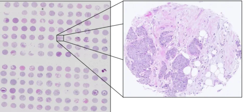
1.1 Example of a tissue microarray with a single core magnified . . . 2
2.1 Stain normalization. . . .14
2.2 Overview of hierarchical dictionary learning . . . .14
2.3 Overview of Zero-phase Component Analysis . . . .15
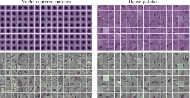
2.4 Dictionary elements learned on nuclei-centered and dense patches. . . .22
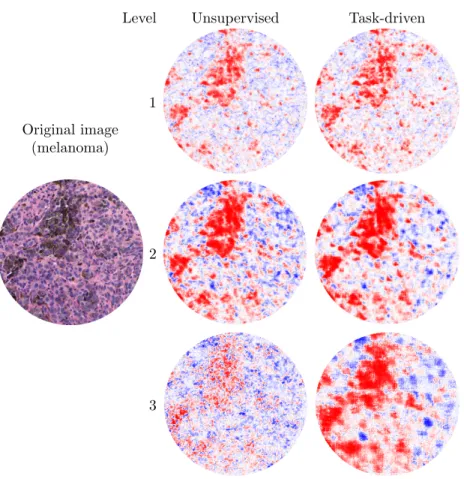
2.5 Relevance maps for a sample image . . . .27
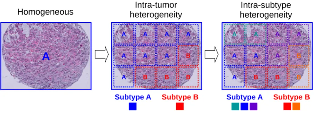
3.1 Intra-tumor and intra-subtype heterogeneity . . . .30
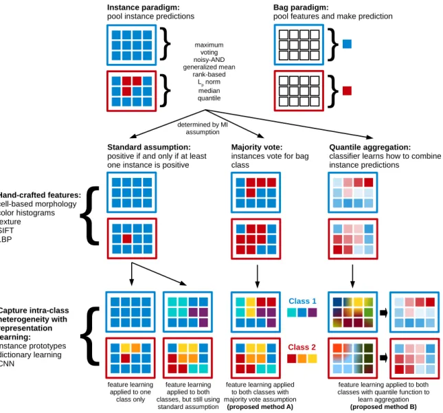
3.2 Related work for MI . . . .31
3.3 Overview of iterative MI method . . . .37
3.4 Process for classifying images with multiple instances and quantile aggregation . . . .38
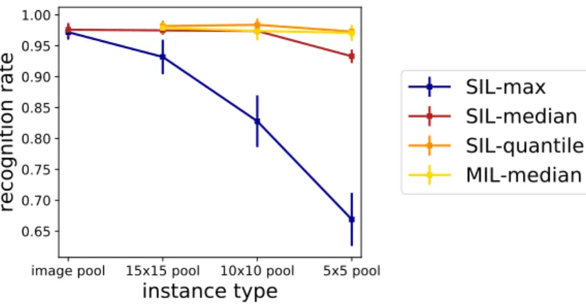
3.5 Recognition rate for different MI methods on the BreaKHis data set . . . .41
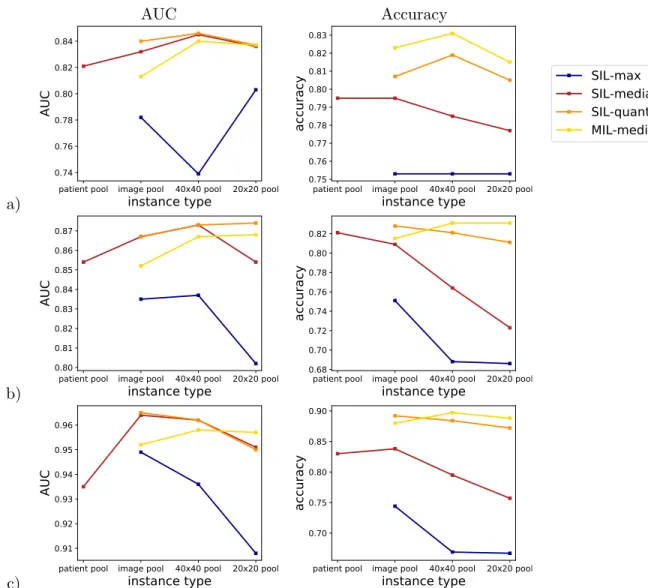
3.6 AUC and classification accuracy for different MI methods on the CBCS data set . . . . .42
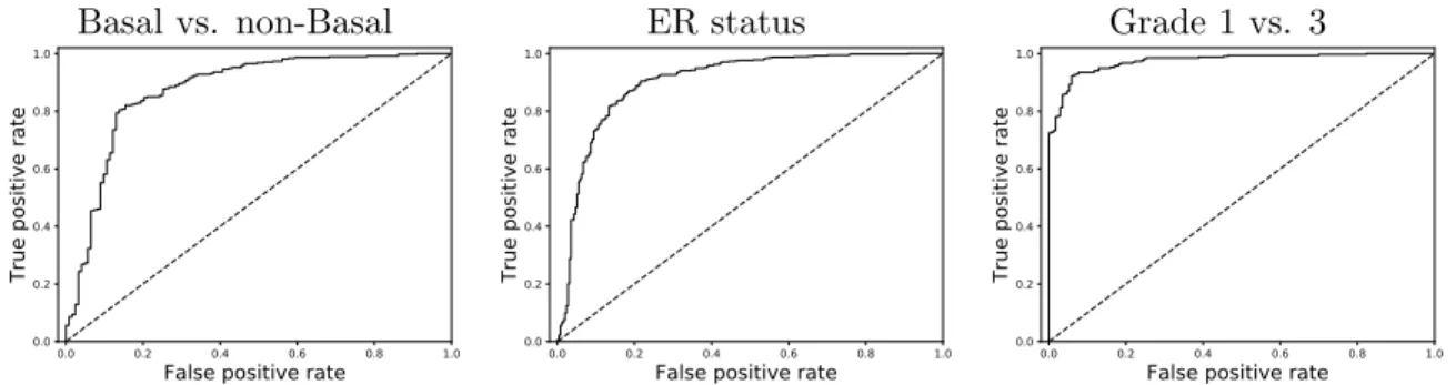
3.7 ROC plots for MIL-median with VGG16 . . . .43
3.8 Predicted tumor heterogeneity across four H&E cores from a single patient . . . .45
4.1 MI augmentation . . . .48
4.2 MI framework with a CNN . . . .50
4.3 Classification accuracy for different cropped image sizes . . . .54
4.4 t-SNE plots of pre-trained vs. fine-tuned CNN features. . . .57
4.5 Visualization of instance predictions . . . .58
4.6 Predicted heterogeneity for grade and genomic subtype . . . .58
5.1 Deep CCA network architectures . . . .65
5.2 Sum correlation vs. classification accuracy for DCCA and SoftCCA. . . .77
5.3 Batch size vs. classification accuracy on MNIST split . . . .78
5.4 Training set size and input dimension vs. classification accuracy on MNIST split . . . . .78
5.5 t-SNE plots for CCA methods on MNIST split. . . .80
CHAPTER 1: INTRODUCTION
Cancer is a heterogeneous disease, comprising multiple subtypes associated with distinctive morphology, genomics, clinical presentations, responses to treatment, and outcomes. Under-standing its diverse nature is critical in tailoring treatments to each patient. Although there are distinct subtypes of cancer, significant intra-tumor heterogeneity still exists in many individual cancers, posing a challenge for diagnosis and treatment. To date, most research has focused on identifying and characterizing distinct subtypes [Paik et al., 2004; Parker et al., 2009], while only more recent interest has been directed at understanding the effects of heterogeneity [Alizadeh et al., 2015; McGranahan and Swanton, 2015].
Understanding cancer requires the use of a heterogeneous mix of data types: clinical, histol-ogy, radiolhistol-ogy, genomics, and proteomics, among others. Each modality provides a complemen-tary view of the same lesion. I target histologic and genomic analysis of breast tumor tissue. Histology images show microscopic views of tissue and enable pathologists to diagnose disease and assess prognosis. However, interpretation by pathologists is limited by its subjectivity, speed, and the capability of humans to discriminate complex properties. Through image anal-ysis, I form automated methods for assessing the prognosis and subtype of tumor tissue, which could lead to better treatment decisions for cancer. Although the focus of this dissertation is on breast cancer, the techniques are generalizable and could provide powerful quantitative analysis methods for many other cancer types and diseases in general.
whereas a full slide is often 50,000 pixels or more in width. Adjacent slices of tissue are stained to identify other tumor properties such as estrogen, progesterone, and HER2 receptor status. Other core samples are sent for genomic analysis, providing the expression level of a set of genes and the genomic subtype. The PAM50 subtype has been shown clinically-relevant and is associated with the tumor receptor status [Parker et al., 2009].
Tumor tissue is far from homogeneous. Different types of heterogeneity may be present: 1) Although tissue cores are taken from tumor tissue, they may contain adjacent stroma (connec-tive) or adipose (fatty) tissue, each with a different appearance and each may or may not be connected with the discrimination task at hand. 2) A single genomic subtype is assigned to each sample, but the tumor may contain a mix of subtypes. 3) Tumors of different histologic types may belong to the same genomic subtype, resulting in a varied appearance for each subtype. Methods to target each of these challenges will be explored.
This dissertation studies ways to learn representations directly from histology images, cap-ture intra-tumor heterogeneity, and integrate image and genomic data to form more predictive models for subtyping, grading, and prognosis. Feature learning is an integral component to each chapter. It is used to represent image patches and sub-regions of an image as instances in multiple instance (MI) learning. A dictionary of image patches can provide a basis for rep-resenting a set of heterogeneous components and aids interpretation as only a small number of dictionary elements are used to reconstruct a sample. More powerful, but less interpretable, features are obtained with a Convolutional Neural Network (CNN). Discriminative models are also essential to each of the frameworks that I work with. Some methods are faster to train,
some are top performers when given a lot of data, and others excel in the high-dimensional low sample size (HDLSS) setting. Classifiers with each of these characteristics will be employed and adapted to the unique properties of histologic images. When combined, feature learning with a discriminative model provides a powerful way to make predictions from heterogeneous data.
1.1 Computer Science Motivations
Discriminative Image Representations. Traditional approaches to image analysis in-volved hand-crafting domain-specific features to describe the color, shape, or texture of im-ages [Julesz, 1981; Gotlieb and Kreyszig, 1990; Miedema et al., 2012]. However, hand-crafted features are difficult to develop and to transfer to new applications. Somewhat more generic hand-engineered features were later invented to characterize local regions of an image [Lowe, 2004; Bay et al., 2008; Dalal and Triggs, 2005], but are not adapted to the needs of a specific image type or application. More recent work in dictionary learning and deep learning forms features directly from the images [Mairal et al., 2009; Le et al., 2012b]. However, most recent advances have focused on forming discriminative features from small images using deep learning [Krizhevsky et al., 2012; He et al., 2016; Szegedy et al., 2017]. Extensions of these methods are necessary to handle large, heterogeneous images and to find subtle differences between image classes that are not visually distinguishable to domain experts.
Multimodal Data Analysis. A variety of cross-modal analysis methods exist, mostly based on Canonical Correlation Analysis (CCA), enabling the projection of two modalities of data to a shared space [Hotelling, 1936; Andrew et al., 2013]. This shared space can then be used for cross-modal classification or other data analysis tasks. While a great deal of effort has focused on maximizing the correlation between modalities in this shared space [Wang et al., 2015a; Chandar et al., 2016; Chang et al., 2018], there has been very little focus on ensuring that the shared space remains discriminative. Task-driven deep CCA methods are needed to find a projection that is both highly correlated and discriminative. By ensuring robustness in the HDLSS setting, such a method can be applicable to medical applications and can further data interpretation efforts.
1.2 Motivations in Cancer Research
Diagnosis and Prognosis. Pathologists examine biopsied or resected tissue to identify the presence of a tumor and to characterize multiple features in order to assess tumor aggressiveness. Accurate diagnosis and assessment of tumors is fundamental in providing appropriate and timely treatment. By improving the accuracy of diagnosis, we can reduce over-treatment of benign lesions and under-treatment of malignant ones. Better survival prediction can help to determine how closely to monitor patients and which patients should be offered entrance into clinical trials.
Genomic Subtypes. Although visual examination of tissue by a pathologist is typically used for diagnosis and grading, genomic subtyping can further guide treatment decisions for the goal of personalized medicine. For breast cancer, intrinsic subtypes are determined through the PAM50 molecular genomic assay, dividing tumors into five classes [Parker et al., 2009]. These subtypes have different prognoses and respond to treatment differently [Parker et al., 2009].
Heterogeneity. Genomic subtypes are assigned from a single sample of tissue; they cannot provide a spatial view of the tumor. Although some tumors are mostly homogeneous, others are very heterogeneous, likely due to their branched evolution [Hiley and Swanton, 2014]. This heterogeneity can lessen the predictive ability when multiple types are present in a single tumor, as the patient would fall into a different subtype dependent on which part of the tumor was sampled. The implications on prognosis and targeted therapies are not yet well understood [Alizadeh et al., 2015]. Histology gives us the ability to examine the spatial heterogeneity of the tumor in a way that gene expression cannot.
Computational Methods for Subtypes. Recent advances in prognostication have relied on molecular and genomic methods that are costly and not routinely performed on all patients who could benefit. Predicting genomic properties from H&E histology alone could identify patients who are most like to benefit from further genomic testing. Further, genomic data is not always available, such as in low resource settings or due to insufficient tissue. In these situations, computational image-based methods could provide a lower cost substitute.
Multimodal Models. Histologic image features and genomics provide two complementary views of tumors. By combining the two, a more complete picture of tumor prognosis and treatment models can be developed. Each alone has been shown to inform certain decisions made by doctors, but an integrated model can provide a more predictive analysis. Initial efforts for breast and prostate cancer show the potential of multimodal methods for outcome prediction [Yuan et al., 2012; Lee et al., 2015].
most contributed to a prediction can create a teaching mechanism for pathologists.
Other Medical Applications. Although my focus is on H&E histology data sets, the tech-niques described in this work are not specific to this type of image. They could provide powerful quantitative analysis methods for many other cancer types and staining protocols and also many other diseases exhibiting heterogeneity, such as chronic obstructive pulmonary disease (COPD) [Mannino, 2002; Agusti et al., 2010] and Alzheimer’s disease [Lambert and Amouyel, 2007].
1.3 Thesis Statement and Contributions
Learned representations for histology images of tissue can capture both intra- and
inter-tumor heterogeneity, enabling discriminative models for inter-tumor properties. Combining these
image features with data from other modalities such as genomics in a task-driven model can
provide insight into the shared tumor properties and further improve predictions. These
compu-tational techniques using discriminative features can provide a lower cost and more repeatable
alternative to molecular methods and insight into tumor heterogeneity.
The contributions of this dissertation in Computer Science include:
1) Discriminative representations for histology images using dictionary learning or deep transfer learning. The dictionary learning method is task-driven to discover subtle dif-ferences between classes and hierarchical to capture architectural properties. The deep transfer learning method validates the use of pre-trained CNN features for discriminative tasks on non-RGB images.
provided by visualizing the predictions of each instance.
3) A set of multimodal methods to find a shared space that is also discriminative. This set of deep CCA models can be used for cross-modal classification and in gaining insight into the shared components of two modalities. They bring the CCA projection into the network itself in different ways, enabling end-to-end training to optimize both the correlation between modalities and the task-driven goal.
4) Techniques for deep learning on problems traditionally viewed as “small data.” Solutions in this regime include deep transfer learning, multiple instance learning on large images, multi-task learning, and appropriate regularization.
Further contributions to the application area of breast cancer research include:
A) Methods to capture biologically-relevant features by operating on the H&E stain intensities extracted from histology images. These methods do not rely on hand-crafted features and are shown to produce more accurate predictions. The feature learning methods are also easily transferable to other cancer types.
B) A low cost and repeatable method for predicting histopathological, molecular, and genomic properties of tumors from H&E histology. Experimental validation shows that the clas-sification accuracies achieved are comparable to the inter-rater agreement of pathologists and of alternative ways of assessing tumor properties. Further, these methods showed success on predicting molecular and genomic properties from H&E histology - something not previously known to be possible from H&E alone.
1.4 Overview of Chapters
CHAPTER 2: REPRESENTING HISTOLOGY IMAGES
Appropriately representing images is the first and most critical step in applying automated analysis. The features must capture the important properties of the image for the chosen dis-crimination task. In the case of predicting diagnosis, prognosis, or subtype, the class differences can be very subtle. Machine learning methods perform such tasks by first representing images by a vector of features. Traditionally, these were hand-crafted features describing the color, shape, or texture of the image [Julesz, 1981; Gotlieb and Kreyszig, 1990; Tuceryan and Jain, 1998; Miedema et al., 2012] or hand-engineered features capturing properties of local image patches [Lowe, 2004; Bay et al., 2008; Dalal and Triggs, 2005]. A classifier then maps each feature vector to a class prediction, such as normal versus disease [Lepist¨o et al., 2003; Varma and Zisserman, 2005; Csurka et al., 2004].
Histological image analysis presents many challenges due to variations in staining and bi-ological heterogeneities [Niethammer et al., 2010]. Each tissue type has specialized structures [Young et al., 2013], making hand-crafted features developed for one type difficult to apply to another. Tumors from different genomic subtypes may also appear similar, requiring features that capture their subtle differences. Rather than engineering specific features for each data type and task, a representation can be learned directly from the data [Varma and Zisserman, 2007; Coates et al., 2010; Coates and Ng, 2011]. Dictionary learning and deep learning are two such methods that I explore in this chapter.
2.1 Overview of Representations
Hand-crafted Cell Features. Several previous studies have utilized automated processing of H&E stained breast tumors to identify image features associated with tissue types or outcome. They generally follow an approach of first segmenting nuclei, then characterizing color, texture, shape, and spatial arrangement properties of cells and nuclei [Miedema et al., 2012; Cooper et al., 2012; Chang et al., 2011]. A simple averaging of cell and nuclear properties in a region of tissue has limitations due to its focus on local properties of cells. Further, these hand-crafted features are time-consuming to develop and do not adapt easily to new data sets. Prior work on automated grading addresses mitotic count [Veta et al., 2015], nuclear atypia [Khan et al., 2015], and tubule formation [Basavanhally et al., 2011] individually; however, the latter two require a nuclear segmentation that is also difficult to adapt to new data sets.
Hand-engineered Patch Descriptors. Other more general feature descriptors developed for other types of images have also been applied to histology. Cruz-Roa et al. compare greyscale image patches, the Scale Invariant Feature Transform (SIFT), the Discrete Cosine Transform (DCT), and Local Binary Patterns (LBP) [Cruz-Roa et al., 2011, 2014]. Although these and other features have great utility on many image analysis problems, they are not optimal for histology or many other fine-grained image classification tasks [Cruz-Roa et al., 2013, 2014].
digits [Mairal et al., 2012]. I extend it to a hierarchical dictionary learning framework for classifying large images.
Dictionary learning is computationally-intensive in both learning the dictionary during training and computing coefficients at test time because it requires an optimization process rather than a feed-forward computation. For this reason, I implemented the encoding function for processing on a Graphics Processing Unit (GPU). The complexity of the computation is also a problem during training; therefore, I implemented the hierarchical framework in a greedy manner, learning one layer at at time.
Deep Learning. Deep learning is a method of learning a hierarchy of features where the higher level concepts are built on the lower level ones [LeCun et al., 2015]. Automatically learning these abstract features enables the system to learn complex functions mapping an input to an output without the need for hand-crafted features. In comparison to dictionary learning, deep learning is much more efficient and can thus be scaled to larger models. Highly optimized software is commonly available for training and testing convolutional neural networks (CNNs) on a GPU. While the encoding function for each layer is simpler than for dictionary learning, the power comes from stacking many layers into a larger model with end-to-end training.
The largest downside of deep learning is the limited interpretability of these large models. Methods have been developed to identify which regions of an image are important for classifica-tion [Simonyan et al., 2013; Bach et al., 2015] or visualize individual features [Zeiler and Fergus, 2014], but this is still very much an active research area. In Chapters 3 and 4 I will develop heatmaps to identify which regions of an image are most associated with its class. Gaining insight into individual features is not tackled in this dissertation but will be important in the future, particularly as deep learning is increasingly applied to medical applications.
2013] and for specific tasks such as mitosis detection [Cire¸san et al., 2013; Veta et al., 2015], tissue segmentation [Xu et al., 2016], and segmentation and detection of a number of tissue structures [Janowczyk and Anant, 2016].
Many state-of-the-art CNN models are trained with tens or hundreds of millions of labeled images. In the medical domain, expert annotations are expensive and patient samples are scarce. Training a large model on a small data set may result in overfitting - the model performs well with the data it was trained on but gives poor results on newly presented data [Cawley and Talbot, 2010]. This is because the model has too many parameters relative to the amount of labeled data. Predicting diagnosis, subtype, prognosis, or other such complex classes uses patient-level labels, making it much more difficult to obtain large quantities of labeled data. End-to-end training of a CNN will be addressed in Chapter 4. In this chapter, I use a pre-trained CNN for transfer learning.
Transferred Deep Features. To accommodate the limitations of small data sets, deep learn-ing models trained on more general image data sets can be transferred to specific applications. Typically, the network is transferred at some intermediate layer, and either the network is fine-tuned on the new data or the transferred layer of features is used to train a new classifier. The former has shown a lot of success for fine-grained classification tasks that have larger amounts of labeled data [Yosinski et al., 2014; Azizpour et al., 2014; Zhang et al., 2015]. The latter has been applied to tasks with smaller data sets and can still outperform hand-engineered features [Zhang et al., 2015; Codella et al., 2015; Donahue et al., 2014]. Transferability is less for distant tasks, particularly for higher layers due to their specialization [Yosinski et al., 2014], making this technique even more difficult to apply to a specialized image set such as histology.
examples [Shouno et al., 2015]. Each of these applications still has many more labeled samples than the data sets that I work with. I study the use of a large pre-trained CNN in extracting features for classifying histology images.
Applications on Histology. Significant advances in image analysis for histology have shown promise for tumor detection [Cruz-Roa et al., 2013], metastatic cancer detection in lymph nodes [Wang et al., 2016a], mitosis detection [Veta et al., 2015; Cire¸san et al., 2013], tissue segmentation [Xu et al., 2016], and segmentation and detection of a number of tissue structures [Janowczyk and Anant, 2016]. However, all of the previous successes of deep learning from H&E images have focused on detecting image-based properties that pathologists routinely assess visually. Using deep learning to predict complex properties that are not visually apparent to pathologists, such as receptor status or genomic subtype, has not been previously described. I tackle predicting both types of tumor characteristics.
2.2 Stain Normalization
Staining of tissue samples is commonly used to highlight structures of interest, with hema-toxylin and eosin as the most commonly-used set for histological diagnosis. Hemahema-toxylin turns nuclei blue and eosin turns cytoplasm pink. Standardization of slide appearance can help to counter variations due to slide fading, differing stain colors, and the variety of microscopes and imaging equipment used. Color and intensity normalization helps to minimize these variations by estimating the stain vectors for hematoxylin and eosin and normalizing each image.
I use the method by Niethammer et al. [Niethammer et al., 2010] that uses prior information on the absorption coefficients for each stain in order to provide support for images with sparsely distributed nuclei. The image is decomposed into the components of each individual stain using color deconvolution. The resulting stain intensity channels are then used as input to the rest of my algorithm. An example is shown in Figure 2.1.
2.3 Dictionary Learning1
1The methods presented in this section were presented at the IEEE International Symposium on Biomedical
a) b) c)
Figure 2.1: Stain normalization: a) original H&E image, b) stain normalized, c) stain intensities with hematoxylin in the red channel, eosin in the green channel, and the residual in the blue channel.
dictionary
encoding pooling
pooling encoding
. . .
level 1 level 2
D1
D2
α1 α2
max max
≈ 0.2 +0.2 +0.1 +0.5 =[0,…,0.1,…,0.2,…,0.2,…,0.5,…,0]
input image
Figure 2.2: Overview of hierarchical dictionary learning: Images are first color normalized and the hematoxylin, eosin, and residual stain channels extracted. Each image patch is encoded using a dictionary. Following encoding, a max pooling operation downsizes the image. By alternating encoding and pooling layers, a hierarchy of features is formed.
Dictionary learning based on sparse coding can learn representations for histology images. A dictionary is learned from image patches in the training set, which is then used to encode patches in novel images. This section outlines the steps to learn hierarchical task-driven dictionaries and apply them to encode images for classification. Whitening is first used to decorrelate image patches. Figure 2.2 provides an overview of this hierarchical process of image encoding.
original decorrelated
original PCA-whitened ZCA-whitened
rotate rescale rotate back
Figure 2.3: Overview of Zero-phase Component Analysis (ZCA). Computed using SVD, three operations are performed: a rotation to decorrelate the data, a rescaling of each axis, and a rotation back to the original space.
features uncorrelated and to give each feature a similar variance [Hyv¨arinen and Oja, 2000; Mairal et al., 2014]. Whitening has previously been found to improve image classification accuracy when applied as preprocessing [Coates et al., 2010]. This centering and whitening process is applied prior to encoding for each level of the hierarchy.
A set of n image patches, each flattened into a d-dimensional vector, is stored in matrix XRd×n (n >> d) and mean centered. Whitening applies a transformation ˜X =U X to make
˜
XRd×n orthonormal: ˜XX˜T =I. The covariance matrix ofX is computed as C = n−11XX
T. Any matrix U Rd×d that satisfies the condition UTU = C−1 whitens the data; however, U
is only defined up to a rotation, so it is not unique. I first apply PCA whitening to decorre-late the features, followed by a rotation back to the original space. PCA whitening uses the eigendecomposition of covariance matrix C: UP CA = Λ−1/2VT for Λ = diag(σ1, ..., σd) and
V = [v1, ..., v1], where (σi2, vi) are the eigenvalue, eigenvector pairs of C. ZCA uses the trans-formationUZCA=VΛ−1/2VT, in which PCA whitening is first applied, followed by a rotation back to the original space. While PCA is commonly used to reduce the data dimensionality, ZCA typically keeps all d dimensions. Adding the rotation V brings the whitened data ˜X as close as possible to the original input data X [Kessy et al., 2015]. An overview of ZCA whitening is shown in Figure 2.3.
where dictionary elements are similar. Given whitened input data {x1, ..., xn}, xiRd, the goal
is to compute a dictionary DRd×k and coefficients {α1, ..., αn} such that the reconstruction errorPn
i=1||xi−Dαi||2 is minimized and the coefficients αare sparse.
If the dictionary Dis known, the coefficients α can be computed by optimizing
α∗(x, D) = argmin α
1
2kx−Dαk
2
2+λ1kαk1+λ2kαk22. (2.1)
The `1 norm encourages sparsity in α, and the`2 norm adds stability in the case of correlated
variables. Due to the computationally intensive nature of evaluating the elastic net, I perform this on a GPU.
Initially, the dictionary D must be learned from the data. It is computed from a set of whitened image patches{x1, ..., xn}after first initializing with random patches. I use a similar elastic net formulation in which both the coefficientsα and the dictionary Dmust be learned:
D, α= argmin D,α
1 n
n
X
i=1
1
2kxi−Dαik
2
2+λ1kαik1+λ2kαik22
such that for each column of D,kD:,jk22 ≤1. Although this cost function is not convex, it can
be split into the sub-problems of optimizing for the dictionary Dgiven the coefficients α, and optimizing for the coefficientsα given the dictionaryD. Each of these sub-problems is convex, so the typical approach is to alternate the two steps until convergence. I use the online batch implementation by Mairal et al. [Mairal et al., 2009].
Task-Driven Dictionary Learning. The discriminating power of the dictionary can be improved by incorporating image label information into the dictionary learning framework [Mairal et al., 2012]. By minimizing the logistic loss, I learn a linear discriminant for two classes based on the sparse encodings of individual image patches. Although I focus on binary classification here, the logistic could be replaced with the softmax function to generalize to multiple classes.
separating hyperplane w such that if wTα∗(x, D) +w0 > 0, patch x is predicted to belong
to class 2, and class 1 otherwise. The logistic function 1/[1 +e−(wTα∗(x,D)+w0)] predicts a
probability indicating how likely the patch is to belong to class 2.
In improving the dictionary and classifier, the logistic loss objective function I use is as follows:
f(D, w) = min w,D
n
X
i=1
log[1 +e−yi(wTα∗(xi,D)+w0)] +ν
2kwk
2 2
whereyi is the class label (-1 or 1) associated with each patchxi,wdefines the hyperplane sepa-rating the two classes,α∗(x, D) is defined in (2.1), and parameterν controls the regularization. I optimize this objective by stochastic gradient descent, updating Dand was
D←D−γODf(D, w) w←w−γOwf(D, w)
where γ is the learning rate, and Owf(D, w) and ODf(D, w) are calculated from the logistic loss functionf(D, w) usingODα∗(x, D) derived by Mairal et al. [Mairal et al., 2012].
Hierarchy of Features. Now that I can form dictionaries of learned features and use them to encode images, I turn to the problem of forming a feature hierarchy to capture more abstract and larger scale properties. After densely encoding every patch in an image, a max pooling operation is applied in which, for each m×m region, I take the maximum encoded value for each feature. This has the effect of providing local translation invariance and downsizing the representation to enable capture of larger-scale properties by the next level. Encoding and max pooling operations are alternated to form a feature hierarchy.
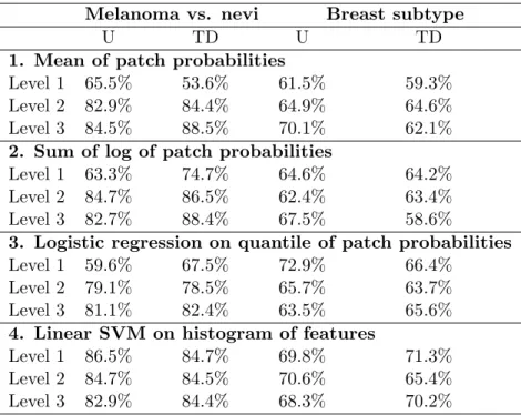
Classification. At this point, each image is represented by a set of sparse encodings of features from each level of the hierarchy and I must predict the image-level class. I can apply the logistic regression classifier to each image patch or summarize the encodings themselves and train a new classifier. I compare four image-level classification methods:
1) The mean of the patch probabilities over the image.
3) A new logistic regression classifier to operate on quantile functions summarizing patch probabilities.
4) A Support Vector Machine (SVM) to operate on histograms of the patch encodings (equiv-alent to a mean pool of the encodings).
For the first two options, I found it to work best if a threshold to separate the two classes is learned on the training data. I experiment on each of these strategies in Section 2.5.5.
Summary. This section presented dictionary learning in a task-driven and hierarchical frame-work. The task-driven component increases the discriminability of dictionary elements while the hierarchical part captures larger-scale and more abstract features, such as tissue architec-ture. Task-driven dictionary learning has previously been applied to small images [Mairal et al., 2012]; I applied it to patches within a larger image and proposed four aggregation schemes for image classification. I also extended task-driven dictionary learning from a single layer to a multi-layer hierarchy.
2.4 Deep Transfer Learning
CNNs consist of convolution filters applied to small patches of the image, followed by a non-linearity and often a data reduction or pooling layer [LeCun et al., 2015]. Convolutional and pooling layers are typically alternated to extract features and provide local translational invariance, respectively [Krizhevsky et al., 2012; Simonyan and Zisserman, 2015]. Fully con-nected layers may be added on top of the convolutional network, and a softmax regression layer is applied for classification. Backpropagation is used to learn the network parameters. Similar to human visual processing, the low level filters detect small structures such as edges and blobs. Intermediate layers capture increasingly complex properties like shape and texture. The top layers of the network are able to represent object parts like faces or bicycle tires. The network weights are learned from data, creating discriminating features at multiple levels of abstraction. There is no need to hand-craft features.
consists of 1.2 million images from 1000 categories of objects and scenes. Although ImageNet contains a vastly different type of image, CNNs trained on this data set have been shown to transfer well to other data sets [Oquab et al., 2014; Razavian et al., 2014; Yosinski et al., 2014], including those from biomedical applications [Wang et al., 2016a; Tajbakhsh et al., 2016]. The lower layers of a CNN are fairly generic, while the upper layers are much more specialized. The lower layers only capture smaller-scale features, which do not provide enough discriminating ability, while the upper layers are so specific to ImageNet that they do not generalize well to histology. Intermediate layers are both generalizable and discriminative for other tasks.
In transferring to histology, I search for the layer that transfers best to a particular task. I extracted the output from each layer over each image at full resolution to form a set of features for the image. Taking the mean of each feature over the tissue region (excluding the background), then forms a single feature vector for each image - essentially a weighted global mean pool with weights of one where there is tissue and zero for the background. When multiple images are available for each patient, I further average across images.
The ImageNet data set on which the CNNs were pre-trained consists of RGB photographs of scenes and objects. H&E histology images contain a much more limited set of colors and appearances with their focus on the blue/purple color of nuclei with hematoxylin staining, the pink color of surrounding tissue with eosin staining, and the remainder mostly white. While the stain-normalized RGB images of histology provide one view, I also experiment with the decomposition into hematoxylin, eosin, and residual. I use these three channels as input by first subtracting a per-channel mean across the data set and then extracting features with a pre-trained CNN. Experimental results comparing feature learning strategies and assessing stain normalization for preprocessing are in Sections 2.5.3 and 2.5.4, respectively.
2.5 Experiments
normalization, and 3) hierarchical task-driven dictionary learning.
2.5.1 Data Sets
Melanoma. The melanoma data set consists of whole slide images in which a pathologist has annotated an average of eight regions containing tumor. 31 of these samples contain varying degrees of dysplastic nevi (benign), while 21 contain melanoma.
SPECS. My second data set contains breast tumor samples from a Washington University cohort of patients [Parker et al., 2009]. These take the form of a tissue microarray with two cores per patient; they were imaged at the University of British Columbia. I predict the subtype of the 43 Basal and 42 Luminal A samples.
CBCS. This data set consists of 1713 patient samples from the Carolina Breast Cancer Study, Phase 3 [Troester et al., 2018]. There are typically four cores per patient (5970 cores total), with each core image having a diameter of around 2400 pixels. I predict Basal vs. non-Basal intrinsic subtype, ER positive vs. negative, and grade 1 vs. 3.
2.5.2 Implementation Details
Deep Transfer Learning. Features were extracted using the AlexNet CNN pre-trained on ImageNet [Krizhevsky et al., 2012]. The mean output of the fourth convolutional layer over the tissue region was taken for each image and further averaged over all images for each patient.
Dictionary Learning. A patch size of 17×17 and dictionary size of 256 was used for unsupervised dictionary learning. I selected λ1 from 0.25, 0.5, 1.0, and 2.0 as the value that
produced the best patch classification accuracy through cross-validation on the training set. I setλ2 toλ1/10 to add some stability to the model, while keeping the`1 norm as the main mode
of regularization. The mean of the computed coefficients from overlapping patches was taken for each image and further averaged over all images for each patient.
3×3 max pool for each. Dictionary learning requires setting the regularization parametersλ1
and λ2 (Section 2.3). I selected λ1 from 0.25, 0.5, 1.0, and 2.0 as the value that produced the
best patch classification accuracy through cross-validation on the training set. I once again set λ2 toλ1/10 to add some stability to the model, while keeping the `1 norm as the main mode
of regularization. The logistic loss of task-driven dictionary learning requires a regularization parameterν (Section 2.3). I also learned this from the data as the value from 10−6 to 101 that produced the greatest patch classification accuracy. During learning, patches were randomly selected from each image and were randomly flipped and/or rotated to add more variety to the data. A learning rate γ of 10−5 was found to work with my data sets in combination with a batch size of 500000/N patches from each image, where N is the number of training images; 60, 20, and 15 cycles through the training set were used for the three levels respectively.
Classifier Hyperparameters. Hyperparameters for logistic regression, SVM, and DWD were learned through cross-validation on the training set to maximize the area under the ROC curve (AUC).
2.5.3 Unsupervised Feature Comparison
Using the SPECS data set, I compared different methods of unsupervised feature learning. Feature representations for the training images were learned without the class labels, followed by encoding the images in the learned representation and training a classifier using the class labels. The AUC was computed as a measure of accuracy for each method and is presented in Table 2.1 as the mean over two rounds of five-fold cross-validation. The hand-crafted features used are described by Miedema et al. and capture the size, shape, stain intensity, texture, and local spatial arrangement of cells and nuclei [Miedema et al., 2012]. Dictionary learning was run on nuclei-centered patches and dense overlapping patches; Figure 2.4 shows the dictionary elements that were learned. A pre-trained CNN was also compared by taking the outputs from the fourth convolutional layer of AlexNet [Krizhevsky et al., 2012].
lay-Method Log. Reg. SVM - Linear SVM - RBF DWD Hand-crafted features 78.9% (3.2) 77.8% (2.7) 57.3% (4.0) 72.8% (2.2) Nuclei-centered patches 81.2% (2.0) 79.4% (1.7) 66.1% (4.5) 75.5% (3.5) Dense patches 84.5% (2.0) 85.5% (2.4) 63.1% (3.5) 79.9% (2.3) AlexNet Conv4 83.2% (2.9) 82.5% (3.2) 71.6% (3.9) 81.1% (3.4) Table 2.1: Patient-level AUC results for different unsupervised feature representations and classifiers on the SPECS data set, with the standard error in brackets.
Nuclei-centered patches Dense patches
Input image AUC Accuracy
Basal ER Grade Basal ER Grade
Original RGB 81.0 (0.8) 84.3 (0.9) 90.5 (0.7) 79.0 (1.2) 79.7 (0.9) 82.8 (1.0) Normalized RGB 81.7 (1.0) 85.0 (0.9) 91.1 (1.0) 78.0 (1.0) 79.0 (1.2) 82.1 (1.3) Stain channels 82.2 (1.4) 86.0 (0.8) 92.7 (0.9) 79.5 (1.2) 80.5 (0.9) 84.8 (1.0) Table 2.2: AUC and classification accuracy on CBCS using dictionary learning on the orig-inal unnormalized RGB images, stain normalized RGB images, and extracted stain channels (hematoxylin, eosin, and residual). Standard error is in brackets.
ers from a pre-trained CNN showed very promising results, although not quite as strong as dictionary learning on dense patches. This is in line with Cruz-Roa et al.’s conclusion that a simple model trained on the desired data type is better than a more complex one trained on a disparate data set [Cruz-Roa et al., 2015].
2.5.4 Stain Normalization with Dictionary or Deep Transfer Learning
I studied stain normalization as a preprocessing step to feature learning. The experiments in this section use the CBCS data set and 5-fold cross validation. The mean and standard error across the five folds is reported.
Table 2.2 compares the classification performance with dictionary learning on the original RGB histology images, stain normalized RGB, and the extracted stain channels (hematoxylin, eosin, and residual). Dictionary learning with the stain normalized RGB images was generally better than with the original histology images. Using the stain channels however, consistently outperformed the other two input image types.
Input image AUC Accuracy
Basal ER Grade Basal ER Grade
Original RGB 78.4 (1.7) 81.9 (0.9) 90.6 (1.4) 77.5 (1.3) 76.7 (0.6) 81.9 (1.3) Normalized RGB 80.7 (1.3) 85.7 (1.1) 92.8 (0.5) 78.4 (1.4) 79.2 (1.0) 84.8 (0.6) Stain channels 012 78.5 (1.5) 85.1 (0.8) 93.3 (0.9) 77.8 (1.5) 79.8 (0.9) 84.2 (1.5) Stain channels 021 78.0 (1.4) 83.3 (0.7) 92.4 (0.9) 77.7 (1.3) 79.2 (0.6) 83.2 (1.1) Stain channels 102 77.3 (1.7) 84.2 (1.2) 92.7 (1.2) 77.3 (1.2) 78.5 (1.0) 84.2 (1.0) Stain channels 120 79.8 (1.4) 84.0 (0.8) 91.7 (1.1) 78.6 (1.5) 79.0 (0.9) 83.5 (0.9) Stain channels 201 76.7 (1.2) 83.7 (1.1) 92.5 (0.6) 77.7 (1.2) 78.4 (0.9) 84.5 (0.9) Stain channels 210 77.8 (1.8) 84.9 (0.2) 92.7 (0.9) 77.4 (1.4) 79.7 (0.8) 83.2 (0.4) Table 2.3: AUC and classification accuracy with deep transfer learning for the original unnor-malized RGB images, stain norunnor-malized RGB images, and different channel permutations on extracted stain channels (hematoxylin, eosin, and residual). Standard error is in brackets.
representation of the image (e.g., by permuting the color channels and again extracting features with AlexNet) would no longer exhibit the same discriminability. This is shown to not be the case, indicating that it is not the individual features captured by the pre-trained CNN providing the discriminative power but the space that they span.
The stain normalized RGB images and extracted stain channels do, however, outperform the original unnormalized RGB images for ER status and grade, but not for Basal vs. non-Basal. This might indicate that ER status and grade distinctions are based on color, but Basal vs. non-Basal is learned from other properties. The dictionary learning results in Table 2.2 also show a similar outcome in that the increase in classification performance due to stain normalization is greater for ER status and grade than for Basal vs. non-Basal.
Tables 2.2 and 2.3 also provide a comparison of unsupervised dictionary learning and deep transfer learning on the larger CBCS data set. While Basal vs. non-Basal was more successful with dictionary learning, ER status and grade 1 vs. 3 performed about equally well with the two methods. Task-driven dictionary learning (this chapter) and fine-tuning a CNN (Chapter 4) can provide further improvements for classification. A larger CNN such as VGG16 [Simonyan and Zisserman, 2015] can also provide more discriminative features.
2.5.5 Hierarchical Task-driven Dictionary Learning2
2The results presented in this section were presented at the IEEE International Symposium on Biomedical
Melanoma vs. nevi Breast subtype
U TD U TD
Level 1 55.2% 59.0% 50.7% 52.0%
Level 2 59.8% 63.9% 56.4% 58.0%
Level 3 59.0% 70.0% 51.1% 54.6%
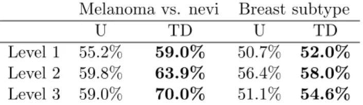
Table 2.4: Patch-level classification accuracy comparing unsupervised dictionaries (U) with task-driven dictionaries (TD) for a 3-level hierarchy.
I assessed both unsupervised and task-driven dictionary learning as a hierarchy by compar-ing the classification accuracy on the melanoma and SPECS data sets.
Classification Results. In order to assess the importance of both the task-driven and hier-archical components of my model, I set up experiments to measure the patch-level and patient-level classification accuracy using 5-fold cross-validation. Although prediction accuracy on patients is expected to be much greater than that on local patches, both provide a means of validation and the latter is important for model interpretation.
First, using the logistic regression classifiers trained during task-driven dictionary learning, I computed the patch-level classification accuracy before and after the task-driven learning pro-cess (Table 2.4). Both data sets showed a consistent improvement of task-driven dictionaries over unsupervised ones. The melanoma data set also showed a consistent improvement from level 1 to 3, with a small decrease in the unsupervised dictionary performance for level 3. The breast subtype results showed a significant drop in performance for level 3 for both methods. This data set is much more complex and poses a more challenging problem. Algorithm param-eters such as patch size and dictionary size likely need to be better tuned to get better results on this data set.
Melanoma vs. nevi Breast subtype
U TD U TD
1. Mean of patch probabilities
Level 1 65.5% 53.6% 61.5% 59.3%
Level 2 82.9% 84.4% 64.9% 64.6%
Level 3 84.5% 88.5% 70.1% 62.1%
2. Sum of log of patch probabilities
Level 1 63.3% 74.7% 64.6% 64.2%
Level 2 84.7% 86.5% 62.4% 63.4%
Level 3 82.7% 88.4% 67.5% 58.6%
3. Logistic regression on quantile of patch probabilities
Level 1 59.6% 67.5% 72.9% 66.4%
Level 2 79.1% 78.5% 65.7% 63.7%
Level 3 81.1% 82.4% 63.5% 65.6%
4. Linear SVM on histogram of features
Level 1 86.5% 84.7% 69.8% 71.3%
Level 2 84.7% 84.5% 70.6% 65.4%
Level 3 82.9% 84.4% 68.3% 70.2%
Table 2.5: Patient-level classification accuracy comparing unsupervised dictionaries (U) with task-driven dictionaries (TD) for a 3-level hierarchy using the four different methods described in Section 2.3.
levels but did not show an improvement from higher levels.
Level Unsupervised Task-driven
Original image (melanoma)
1
2
3
2.6 Discussion
I have studied the performance of different representations in classifying histology images of melanoma and breast cancer. Hand-crafted features are difficult to develop and challenging to adapt to new data sets. Learned features - with dictionary learning or deep learning - produce superior results in classifying tumor tissue.
Deep learning results showed that transfer learning with a pre-trained CNN performed well even on the disparate image type of H&E histology. Further, the non-RGB transformation of extracting stain channels performed equally well, regardless of the channel ordering. This indicates that the power of pre-trained CNN features is not due to the individual features learned, but the space that they span. This conclusion is in line with Szegedy et al. who found that “there is no distinction between individual high level units and random linear combinations of high level units . . . suggest[ing] that it is the space, rather than the individual units, that contains the semantic information in the high layers of neural networks.” [Szegedy et al., 2013] With unsupervised dictionary learning, stain normalization and the extraction of stain channels did provide a measurable increase in classification performance.
CHAPTER 3: MULTIPLE INSTANCE LEARNING FOR HETEROGENEOUS
IMAGES WITH AN SVM1
Automatic classification of histology images can be used to predict diagnosis, grade, or sub-type. For diagnosis, the presence of even a small region of tumor indicates cancer. Tumors can also be grouped into subtypes, but the image may contain a heterogeneous mix of tissue types, making classification challenging as only part of the image is relevant. Tumors of different his-tologic types may also belong to the same genomic subtype, causing heterogeneous phenotypes within a subtype. In addition to classifying the whole sample, quantifying the subtype or other biomarker heterogeneity can provide an important measure for characterizing tumors [Hiley and Swanton, 2014; McGranahan and Swanton, 2015].
Multiple instance (MI) learning is commonly applied for diagnosis by breaking a large image or multiple images into smaller regions [Kandemir and Hamprecht, 2014; Xu et al., 2014a,b]. All data from a particular patient is referred to as a “bag” and each image region is called an “instance.” A bag can have many instances. Labels of cancer and non-cancer are available at the patient or bag level, not the instance level, making this a weakly supervised learning problem. With the standard MI assumption, a sample is classified as positive if at least one of its instances is positive and negative otherwise. This asymmetric relationship works well for diagnosis, but not for problems such as subtype classification in which there is no distinctive “positive” and “negative” class. Diagnosis also requires that the presence of even a small region of tumor should produce a classification of tumor. For histologic and genomic subtypes, it is more appropriate to assign a label to an image based on the properties of multiple regions.
Motivated by the problem of tumor subtyping, I explore MI methods that can treat classes symmetrically and address tumor heterogeneity. These methods enable bag-level predictions as well as instance-level, providing a critical means for interpreting the classification model. Figure
1
Intra-tumor
heterogeneity heterogeneityIntra-subtype
A A A A
A A A B
A B B B
A A A A
A A A B
A B B B
A
Homogeneous
Subtype A Subtype B Subtype A Subtype B
Figure 3.1: The proposed model handles intra-tumor heterogeneity by applying MI learning to multiple regions of an image using a feature set than can capture intra-subtype heterogeneity.
3.1 demonstrates the goals of this work in capturing intra-tumor and intra-subtype heterogene-ity. Breaking a single image into multiple samples accommodates intra-tumor heterogeneity and also increases the amount of training data, which is critical when training data is limited in cancer research and many medical applications. Intra-subtype heterogeneity is handled with the use of an appropriate feature set that can capture the variety of appearances of a single class. Pre-trained CNN features are used in this chapter, although a different feature set, such as dictionary learning (Chapter 2), can also fit into this framework. Fine-tuning a CNN for the MI framework will be discussed in Chapter 4.2.
In this chapter, I examine two simple techniques for adapting MI learning to histology images: 1) selecting an appropriate function to aggregate instance predictions for histology classification (Section 3.2) and 2) generating optimally sized image regions from larger images (Section 3.3). I also propose two new methods to further the state of the art in MI learning: 1) an iterative method for learning latent instance labels under different MI assumptions (Sec-tion 3.4) and 2) aggregating instance predic(Sec-tions with a quantile func(Sec-tion (Sec(Sec-tion 3.5). The implementation discussed in this chapter using an SVM can accommodate any type of image feature.
3.1 Related Work
}
maximum voting noisy-AND generalized meanrank-based Lp norm
median quantile
}
}
}
Bag paradigm:pool features and make prediction
Instance paradigm:
pool instance predictions
determined by MI assumption
Standard assumption:
positive if and only if at least one instance is positive
Majority vote:
instances vote for bag class Hand-crafted features: cell-based morphology color histograms texture SIFT LBP Capture intra-class heterogeneity with representation learning: instance prototypes dictionary learning CNN Class 1 Class 2
{
{
feature learning applied to oneclass only
feature learning applied to both classes, but still using
standard assumption
feature learning applied to both classes with majority vote assumption
(proposed method A)
Quantile aggregation:
classifier learns how to combine instance predictions
feature learning applied to both classes with quantile function to
learn aggregation
(proposed method B)
Reduction to Single Instance Learning. Many image classification solutions for histology and other data types turn the problem into a fully supervised one by representing each bag as a single feature vector [Chen and Wang, 2004; Chen et al., 2006] or applying a specialized kernel [Zhou et al., 2009]. This class of methods can only make predictions at the bag level, not the instance level, so is not suitable for characterizing tissue heterogeneity or interpreting results. The methods that I present make use of an instance classifier.
Instance-level Methods. Rather than making decisions at the bag level, other MI ap-proaches design classifiers to operate on individual instances and then aggregate their output scores or decisions. Andrews et al. developed mi-SVM, in which they apply an SVM to MI learning by iteratively learning the latent instance labels while enforcing the standard MI as-sumption [Andrews et al., 2002]. This class of score- or decision-level fusion methods is able to make use of a larger number of samples drawn from the set of instances when training the classifier. However, mi-SVM still follows the standard assumption: treating classes asymmet-rically. I use the power of mi-SVM in learning latent instance labels but adapt it for a wider range of possible MI assumptions (Section 3.4).
MI Assumptions. For the standard MI assumption, all instances in a negative bag are negative and at least one instance in each positive bag is positive. This asymmetric definition treats positive bags differently than negative. MI techniques have been applied to histology for distinguishing images containing cancer from those that are cancer-free, using the standard assumption [Kandemir and Hamprecht, 2014; Xu et al., 2014a,b]. This asymmetric definition is not appropriate for classifying tumors by subtype. I propose a more general MI assumption in which a given percentage of instances must be positive and a method to learn the latent instance labels. Further, I propose the quantile function as a method for learning to aggregate instance predictions and for use when a suitable MI assumption for a particular task is unknown.
showing that the correlation varies widely by data set domain, learner assumptions, and perfor-mance measures [Vanwinckelen et al., 2016]. They also compared MI methods with their single instance (SI) counterpart, finding that often the SI method outperforms the MI algorithm. In some cases this may be due to a high witness rate - the proportion of positive instances in positive bags [Carbonneau et al., 2017]. To address this, Wang et al. optimize both the bag-level and instance-bag-level loss by including them both in the cost function [Wang et al., 2015b]. My work addresses the challenge of producing an accurate instance- and bag-level classifier by better bridging the gap between them with a more powerful pooling function (Section 3.5).
Image Heterogeneity. Intra-class heterogeneity can be accounted for by forming multiple prototypes for each class; however, initial research in this direction focused on the standard assumption and only applied heterogeneity to the pathological case [Xu et al., 2014b; Li et al., 2015; Wang et al., 2013; Varol et al., 2015]. When each class represents a different subtype of the disease, heterogeneity should be accounted for in all classes. While dictionary learning applied to all classes could address this deficiency, existing methods still remain focused on the standard assumption [Shrivastava et al., 2015; Song et al., 2013; Jiao and Zare, 2015].
3.2 Aggregation Functions for Single Instance Learning
In the following sections, a bag is represented byXn (n= 1, ..., N), has a labelYn{−1,1}, and contains instancesxn,ifori= 1, ..., Mn. The instancesxn,ihave unknown labelsyn,i{−1,1}. A classifier f predicts the class of individual instances, and a function g aggregates these in-stance scores si,n into a bag score Sn:
ˆ
yn,i= sgn(sn,i) sn,i=f(xn,i)
ˆ
Yn= sgn(Sn) Sn=g({sn,1, ..., sn,Mn}).
In the simplest form of MI learning, Single Instance Learning (SIL), all instances are given their bag label and are used to train an instance classifier f. Instance predictions can be aggregated into a bag prediction in different ways. For the standard MI assumption, taking the maximum of all instance predictions is appropriate:
gmax({sn,1, ..., pn,Mn}) = argmax i=1,...,Mn
sn,i.
For many of the classification tasks for histology discussed in this work, the median
gmedian({sn,1, ..., sn,Mn}) = median({sn,1, ..., sn,Mn})
is more suitable. More generally, a given percentile q could be used:
gpercentile({sn,1, ..., sn,Mn}) = percentile({sn,1, ..., sn,Mn}, q).
3.3 Generating Instances
regions ensure that, in the presence of heterogeneity, some of the labeled class is present in each region, enabling more accurate predictions at the instance level. Smaller image regions can result in more training data for the classifier, which is particularly important when labeled data is limited. They also enable predictions to be made on smaller image regions, creating a more interpretable result. The instance size is set by selecting the region size on which to compute features.
3.4 Iterative Multiple Instance Learning
Rather than assigning the bag label to each instance, I propose a method to learn the latent instance labels in order to improve the instance classifier. A particular MI assumption must be chosen corresponding to the aggregation functions discussed in Section 3.2. For the tasks I study in classifying histology images the classes are symmetric, so I chose the assumption that more than half of the instances in a bag must belong to the bag class. More generally, this could be that a given percentage of instances must belong to a particular class.
This MI formulation is based on the linear soft-margin SVM and is an extension of mi-SVM by Andrews et al. [Andrews et al., 2002]. I optimize jointly over the possible classifiers (w, b) and latent instance labelsyn,i with an SVM:
min
{yn,i},w,b,{ξn} 1 2||w||
2+C
N
X
n=1
Mn X
i=1
ξn,i (3.1)
such that yn,i(< w, xn,i > +b) ≥ 1−ξn,i and ξn,i ≥ 0 for all n = 1, ..., N and i = 1, ..., Mn. In order to enforce the aggregation of instances into bags with the correct label, an additional constraint is needed. For the standard assumption with mi-SVM, this is
Mn X
i=1
I(ˆyn,i= 1)>0 if and only if Yn= 1
that a given percentage of instances q must belong to the bag class, expressed as Mn
X
i=1
I(ˆyn,i= 1)≥ q
100Mn for all nsuch thatYn= 1 and Mn
X
i=1
I(ˆyn,i= 1)< q
100Mn for all nsuch thatYn=−1.
(3.2)
For histology, the median is chosen (q= 50).
I use an iterative method to jointly optimize over the possible classifiers and latent instance labels, as outlined in Figure 3.3. The instance labels yn,iare initialized as the class of the bag Yn and are used to train an SVM. Predictions are then made for all instance labels ˆyn,i using the SVM. Instance labels must then be adjusted to meet the constraint (3.2). Instances within each bag are sorted according to the classifier output pn,i. For max aggregation, the highest scoring instance in positive bags is set to +1, while all the instances in negative bags are set to -1. For median aggregation, the instances are first sorted, and then the highest scoring instances in positive bags are set to +1 until half of all instances are positive; the lowest scoring instances are set to -1 in negative bags. The same procedure can be applied for an arbitrary percentile q. These alternating steps are repeated until fewer than 0.1% of instances change label or some maximum number of iterations is reached. The label ˆYn of a novel bagXn can then be predicted as already described in Section 3.2.
3.5 Quantile Aggregation
Prior work has shown that assigning each instance the bag label during training (as in SIL, Section 3.2) can perform quite well in terms of both bag- and instance-level accuracy when the witness rate is fairly high [Carbonneau et al., 2017]; however, bag-paradigm methods still perform better than instance-paradigm methods on some data sets [Wang et al., 2018]. In order to preserve the benefit of an instance-level classifier in providing interpretability but still achieve a high bag-level accuracy, I propose a new method for aggregating instance predictions. This method will also aid applications in which the most suitable aggregator is unknown, as it can learn how much heterogeneity to accommodate.
1) initialize instance labels
2) train classifier 3) predict instance labels 4) adjust instance labels to
meet MI constraints
5) repeat until no instances change label
✗
✓
✓
Figure 3.3: Overview of iterative MI method. 1) Instance labels are initialized according the the bag label. 2) An instance classifier is trained using these labels. 3) The classifier is used to predict the label of each instance. 4) Instance labels are adjusted until the MI constraints are met (e.g., for median aggregation, half of all instances must belong to the bag class). 5) This procedure is repeated until convergence.
function (QF) of instance predictions. Instance predictions are aggregated with the QF, and a bag classifier is trained to predict the bag class from the QF. The QF is the inverse cu-mulative distribution and represents the boundary points between fractions of the population [Broadhurst, 2008]. For random variable X the QF assigns to each probabilitypthe valuexfor which Pr(X ≤x) =p. An instance classifier f is first trained using the bag labels as instance labels. If the instance predictions for bag nare represented by Sn ={sn,1, ..., sn,Mn}, the q-th Q-quantile is the value z such that Pr(Sn ≤ z) = (q−0.5)/Q. To form the QF, I first sort Sn into the set ˜Sn = sorted(Sn). The sorted values in ˜Sn are used to extract the QF vector as Zn = [zn,1, ..., zn,Q], where zn,q = ˜sn,dMn(q−0.5)/Qe. Another classifier g is trained on this bag-level feature set to predict the bag class:
ˆ
Yn= sgn(Sn) = sgn [g(Zn)].
test image
predicted class
instance SVM
CNN features
extract instance features
predict class of instances
compute quantile function
predict image class aggregation SVM CNN
Figure 3.4: At test time, a pre-trained CNN is used to extract features from the image, with a local mean pool to produce each instance. Instance predictions are made with an SVM and a quantile function is used to summarize these predictions over each image. The aggregation SVM then uses the computed quantile function to predict the class of the image.
the QF for each bag. The computed QFs are then used to train the aggregating classifier. This ensemble method ensures that the instance predictions used to train the bag classifier are not biased by being used in training the instance classifier. At test time, the mean of the ensemble predictions on instances is used to form the QF. Figure 3.4 provides an overview of the steps taken to predict the class of a novel image.
The QF captures how much of each class is present in an image, so this technique enables the aggregating classifier to learn how much heterogeneity to expect in images of each class. It can also learn whether the median or some higher or lower quantile is a strong predictor, thus encapsulating many other possible aggregating functions. The QF is more suitable than a histogram as the bin sizes do not need to be specified. It provides a better discretization than a histogram and easily accommodates a non-uniform distribution of predictions from the instance-level SVM. Euclidean distance can be then applied to the QF [Broadhurst, 2008], making the linear kernel still suitable for the bag-level classifier.
3.6 Sample Weighting by Class
When class labels are imbalanced, it is common practice to weight training samples inversely proportional to the frequency of their class label during classifier training. That is, samples of classc are weighting by
wc= N