arXiv:1608.01355v1 [math.PR] 3 Aug 2016
INSIGHTS FROM TRANSITION STATE THEORY
KATHERINE A NEWHALL
Department of Mathematics, University of North Carolina at Chapel Hill
ERIC VANDEN-EIJNDEN
Courant Institute of Mathematical Sciences, New York University
Abstract. This paper is concerned with the long-time dynamics of the nonlinear wave equation in one-space dimension,
utt−δ
2
uxx+V′(u) = 0 x∈[0,1]
where δ > 0 is a parameter and V(u) is a potential bounded from below and growing at least like u2
as |u| → ∞. Infinite energy solutions of this equation preserve a natural Gibbsian invariant measure and when the potential is double-welled, for example when V(u) = 1
4(1−u 2
)2
, there is a regime such that two small disjoint sets in the system’s phase-space concentrate most of the mass of this measure. This suggests that the solutions to the nonlinear wave equation can be metastable over these sets, in the sense that they spend long periods of time in these sets and only rarely transition between them. Here we quantify this phenomenon by calculating exactly via Transition State Theory (TST) the mean frequency at which the solutions of the nonlinear wave equation with initial conditions drawn from its invariant measure cross a dividing surface lying in between the metastable sets. We also investigate numerically how the mean TST frequency compares to the rate at which a typical solution crosses this dividing surface. These numerical results suggest that the dynamics of the nonlinear wave equation is ergodic and rapidly mixing with respect to the Gibbs invariant measure when the parameterδin small enough. In this case successive transitions between the two regions are roughly uncorrelated and their dynamics can be coarse-grained to jumps in a two-state Markov chain whose rate can be deduced from the mean TST frequency. This is a regime in which the dynamics of the nonlinear wave equation displays a metastable behavior that is not fundamentally different from that observed in its stochastic counterpart in which random noise and damping terms are added to the equation. For largerδ, however, the dynamics either stops being ergodic, or its mixing time becomes larger than the inverse of the TST frequency, indicating that successive transitions between the metastable sets are correlated and the coarse-graining to a Markov chain fails.
1. Introduction
Metastability is a feature commonly displayed by dynamical systems [5]. One of its sim-plest manifestation is in the context of finite-dimensional systems whose evolution is governed by the so-called overdamped Langevin equation, that is, steepest descent over a given en-ergy subject to thermal fluctuations modeled by an additive white-noise driving term. In
Date: August 5, 2016.
such systems, if the energy landscape possesses several local minima separated by barri-ers much higher than the available thermal energy, with high probability the solution will spend a long time in a basin associated with the energy minimum before making a transi-tion to another such basin. The time scale of these transitransi-tions follows the Arrhenius law, i.e. it is exponentially large in the energy barrier the system must surmount to escape the basin, measured in units of temperature. This prediction can be confirmed rigorously us-ing Freidlin-Wentzell large deviation theory [13], which also predicts the mechanism of the transitions. More refined estimates for the transition time that include its prefactor can be obtained using e.g. the potential theoretic approach to metastability introduced by Bovier and collaborators [5, 6, 7, 8], and extended by many others [2, 17, 31].
These results can be extended to infinite-dimensional dynamical systems, e.g. the stochas-tic Allen-Cahn equation [3, 11, 31]. They can also be extended to other types of dynamics, e.g. if inertial effects are included. In this case, the system’s evolution can be modeled by the (inertial) Langevin equation, that is, Hamilton’s equations in which a linear damping term and a white-noise forcing term are added in the equation for the momenta. More com-plicated is the case of Hamiltonian systems in which there is no damping nor thermal noise, since the dynamics of such systems is conservative and deterministic. Still, metastability can arise in this context as well. This is most easily pictured in finite dimensional systems, assuming that the constant energy surface the system is evolving upon consists of two large regions connected by a narrow bottleneck: this arises e.g. if the total energy of the system is only slightly higher than the potential energy barrier between two regions in position space. If the dynamics is ergodic, the system can and will eventually cross this bottleneck, but in order to do so it must give up most of its kinetic energy to overcome the potential energy, which is highly unlikely to happen. This picture is intuitively appealing, though it may be hard to justify rigorously since ergodicity is typically very hard to prove. On top of this, it also becomes harder to use and justify as the dimensionality of the system under consideration increases. Indeed, energy typically is an extensive property that grows with the system’s size, meaning that large systems always have much more energy that what is needed to cross a given potential energy barrier. In particular, the picture above seems to become moot for infinite-dimensional Hamiltonian systems, since their total energy can be infinite. The purpose of the present paper is to investigate metastability in the context of one such system.
Specifically, we will study the nonlinear one-dimensional wave equation for u(x, t)
(1) utt−δ2uxx+V′(u) = 0
for x ∈ [0,1], with either Dirichlet or Neumann boundary conditions at x = 0 and x = 1, and V(u) > Cu2 for some C > 0 as |u| → ∞. In (1), δ measures the typical spatial scale
over which u(x, t) varies: this parameter can be absorbed in the domain size after rescaling via ξ=x/δ ∈[0,1/δ]. Defining p(x, t) =ut(x, t), we can write (1) as
(2) ut=p, pt=δ2uxx−V′(u)
which are Hamilton’s equations associated with the infinite-dimensional Hamiltonian (3) H(p, u) =T(p) +U(u),
where
(4) T(p) =
Z 1
0 1 2|p(x)|
2dx, U(u) =Z 1 0
1 2δ
2
We will consider (2) in a parameter regime in which the energy (3) is infinite (in which case we will have to consider weak solutions of (2) – more on this below). In this regime, equation (2) possesses a single natural invariant measure which coincides with the canonical (Gibbs) measure of the associated Langevin system, i.e. the stochastic partial differential equation (SPDE) formally given by
(5) ut=p, pt=δ2uxx−V′(u)−γp+ p
2γβ−1η(x, t),
in which η(x, t) is a space-time white noise, i.e. the Gaussian process with mean zero and covariance E(η(x, t)η(y, s)) = δ(x−y)δ(t−s), γ > 0 is the friction coefficient, and β > 0 is the inverse temperature. The Gibbs measure for (5) can be written formally and in an unnormalized way using the notations of McKean and Vaninsky [20] as
(6) dµ= exp (−βH(p, u))d∞pd∞u.
The precise meaning of this measure will be explained in Sec. 3. The fact that (6) is the only natural invariant measure for (2) is intriguing: indeed, in finite dimensions, Hamilton-ian systems possess two different invarHamilton-iant measures, the microcanonical and the canonical ones, and if their dynamics are ergodic, it can only be so with respect to the former since their evolution is energy-conserving [26]. What therefore happens to the microcanonical measure in the context of the wave equation? The equivalence of invariant measure for the energy conserving wave equation in (2) and its Langevin counterpart in (5) also raises an-other question: Do an-other features of their dynamics coincide, in particular those related to metastability?
We will address both these questions here. Regarding the first, we will consider finite dimensional truncations of the wave equation based on the Hamiltonian defined as
(7) HN(p,u) =
1 N
N X
j=1 1 2p
2
j +V(uj)
+N
N X
j=0 1 2δ
2(u
j+1−uj)2,
where uj = u(xj, t) and pj = p(xj, t) for xj = j/(N + 1), we denote u = (u1, . . . , uN) and p = (p1, . . . , pN), and u0 and uN+1 are fixed by some boundary conditions. These finite
dimensional truncations do indeed possess both the microcanonical and the canonical mea-sures (see (21) and (23) below) as invariant meamea-sures. However we will show in Proposition 1 below thatboth the microcanonical measure on the energy shellEN =N/β and the canonical
measure at inverse temperature β associated with the truncated Hamiltonian in (7) converge to the same canonical measure in (6) as the size N of the truncation tends to infinity. This result will be proven in the context of quadratic potentials V(u) but should hold also for more general potentials. Note that the scaling EN = N/β implies that the energy of the
discretized solutions converge to infinity as N → ∞.
The inverse temperature β in (6) controls the concentration of the invariant measure around the minimizers of the Hamiltonian (3). This concentration of measure suggests that the system’s dynamics can display metastability if V(u) is a double well potential, like e.g. V(u) = 14(1−u2)2, since in that case the Hamiltonian (3) has two minimizers: these are
(p, u) = (0, u−) and (p, u) = (0, u+) where u± are the solutions to
(8) δ2uxx =V′(u)
that minimize the potential energyU(u) defined in (4). ForV(u) = 1 4(1−u
2)2 and Neumann
boundary condition, these are simply u± = ±1, and they can be similarly obtained for
measure in (6) concentrates around these minimizers (0, u±) asβ → ∞, therefore suggesting
that the solutions to (2) spend long periods of time around one before making a transition to the vicinity of the other.
As a means to quantify this behavior and answer the second question raised above, we will compute the mean frequency, averaged over initial conditions drawn from the invariant measure (6), at which the solutions to (2) make transitions between two regions that each contain (0, u−) and (0, u+) and partition its phase-space. Specifically, we will take as the
boundary between these regions the affine set of codimension 1 defined as
(9) S =n(p, u) :R1
0(u−u
s)φsdx= 0o
where us(x) is the saddle configuration between u− and u+, i.e. the solution to (8) with
Morse index 1 that minimizes U(u), and φs(x) is the unique eigenfunction with negative
eigenvalue of the Hessian operator atus, that is
(10) As =−δ2 d
2
dx2 +V′′(u s(x)).
Denoting by NT(p0, u0) the total number of times the solution to (2) for the initial condition
(p(0), u(0)) = (p0, u0) crosses the dividing surface S during the time interval [0, T], T > 0,
we will compute
(11) νS = lim
T→∞
1 2T
Z
NT(p0, u0)dµ(p0, u0)≡ lim T→∞
EµNT
2T .
Transition state theory (TST) [10, 16] permits the exact calculation of this quantity: here we will generalize the derivation in [27] to the wave equation with random initial data to obtain an exact expression for νS that we will then estimate asymptotically in the limit β → ∞. This will allow us to obtain asymptotic expressions for the average residency times τ− and τ+ on either side of S, defined as
(12) τ± = µ(B±)
νS where
(13) B− =n(p, u) :R1 0(u−u
s)φsdx <0o, B
+ =
n
(p, u) :R1 0(u−u
s)φsdx >0o.
The asymptotic expressions for τ± we will arrive at are
(14) τ± ∼2πΛ±eβ∆E± as β→ ∞.
Here, ∆E± =U(us)−U(u±) denote the energy barriers between the minima and the saddle
point and
(15) Λ± = p1
λ±1
∞ Y
j=2 s
λs j
λ±j
where λs
j are the eigenvalues of the operator (10) and λ±j those of
(16) A± =−δ2 d
2
dx2 +V
′′(u±(x)).
In (15) the eigenvalues are enumerated such that λj < λk whenever j < k. Note that the
negative eigenvalue λs
1 < 0 corresponding to the unstable direction of the saddle solution
product. Note also that the infinite product in (15) converges in one spatial-dimension, D = 1, but it does not for D ≥ 2. This issue is consistent with the behavior of the SPDE in (5) which is well-posed for D= 1, but not for D≥2 [15, 25]. Interestingly the prediction in (14) for the residency times of the solutions to (2) coincide with the zero-damping limit of the residency times of the solutions to the Langevin stochastic partial differential equation in (5), since the latter are given by
(17) τ±γ ∼πγ+
p
γ2+ 4|λs 1| p
|λs 1|
Λ±eβ∆E± as β → ∞ with γ >0 fixed.
An interesting additional question is whether these results also apply for almost all initial conditions drawn from the invariant measure. This trajectory-wise comparison is nontriv-ial as it requires an assumption of ergodicity. Below, we will investigate this assumption numerically. These computations suggest that the system’s dynamics is indeed ergodic and rapidly mixing if the parameter δ is small enough: in this case, the residency times of every trajectory closely match that predicted by TST, and successive visits to B+ and B− are
roughly uncorrelated statistically. This means that the dynamics of (2) can be effectively coarse-grained to that of a two-state Markov jump process with rates that can be deduced from the mean TST frequency. It also means that in this regime the dynamics of (2) is not fundamentally different from that of its stochastic counterpart in (5), and in the latter we expect that the limits β → ∞and γ →0 commute. If the parameterδ is too large, however, either ergodicity breaks down, or the mixing time increases and becomes much larger than the inverse of the mean TST frequency. As a result, successive visits in B+ and B− become
strongly correlated, and the coarse-graining of (2) to a two-state Markov jump process fails. In this regime, the dynamics of (2) is different from that of (5), and in this second equation, the limits as β → ∞and γ →0 no longer commute.
The remainder of this paper is organized as follows: In Sec. 2 we begin by setting up the wave equation along with its finite-dimensional truncation that we will study. In Sec. 3 we discuss the equivalence of the microcanonical and canonical distributions in infinite di-mensions, with detailed calculations of the convergence of characteristic functions of the solutions in appendix A and of the concentration of measure in appendix B. In Sec. 4 we then revisit TST and derive the mean frequency of transition between two specific regions in the phase-space of solutions of the wave equation: these calculations are done in main text for initial conditions drawn from the canonical distribution and in appendix C for initial conditions drawn from the microcanonical distribution. In Sec. 5, we confirm these results via numerical calculations and also investigate the ergodicity of the dynamics in different parameter regimes. Finally, in Sec. 6, we conclude the paper by discussing the implications of the Hamiltonian dynamics on the low-damping regime of the Langevin system.
2. Preliminaries: Discretized Equation, Weak Solutions, and Critical Points
To understand the behavior of the solution to (2), we will consider the finite discretization of the interval x∈[0,1], into N + 1 points, defining xj =j/(N + 1), uj =u(xj, t) and pj =
ut(xj, t), and work with the discrete Hamiltonian in (7). Hamilton’s equations associated
with (7) are
forj = 1 toN, where the dot indicates differentiation with respect to time. The Hamiltonian also has 2N degrees of freedom as the endpoints u0 and uN+1 are fixed by the boundary
conditions. For example, u0 = uN+1 = 0 for Dirichlet boundary conditions, oru0 =u1 and
uN+1 =uN for Neumann boundary conditions.
The solutions to (18) converge to those of the wave equation in (2) as N → ∞. However, since we will consider a parameter regime in which the energy of the initial conditions to (18) scale as N/β, the discretized solutions to (18) will converge to infinite energy solutions of (2), and we cannot expect these solutions to be differentiable in space and time. Therefore, we will have to consider weak solution of (2) (or rather (1)) that satisfy
(19)
Z ∞
0
Z 1
0
φtt−δ2φxx
u+V′(u)φ dxdt=
Z 1
0
φ(x,0)ut(x,0)−φt(x,0)u(x,0)dx
for all smooth test functionsφ(x, t)∈C∞ with compact support in time, the same boundary
conditions asu(x, t), and withφt(x,0) = 0.
As mentioned in the introduction, the critical points of the Hamiltonian in (3) will play an important role in what follows. Because of the separable structure of the Hamiltonian, these critical points are always of the form (p, u) = (0, u) with u a solution to (8). The specific shape of these solutions depends both on the form of V(u) and the choice of boundary conditions. To fix ideas, consider e.g.
(20) V(u) = 1
4(1−u
2)2
and Neumann boundary conditions. In this case the solutions of (8) that minimize U(u) in (4) (i.e. such that all the eigenvalues of the operator (16) are positive) are the constant functions u+(x) = 1 and u−(x) =−1.
Besides the minimizers ofU(u), we will also need the saddle point with Morse index 1, i.e. the function us(x) that is a solution to (8) such that the operator (10) has only one negative
eigenvalue. Unlike the minimizers, us(x) as well as its energy Es depend on the value of δ
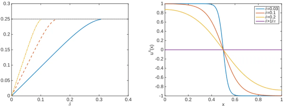
(see Fig. 1 (right)). For instance, u(x) = 0 is always a critical point of the Hamiltonian, but it is only the index 1 saddle point when δ >1/π. This can be seen from the eigenvalues of the operator (10) evaluated at us = 0, namely λ = −1 +δ2n2π2 for n = 0,1,2,3. . .. The
n= 0 eigenvalue is always −1 regardless of the value of δ. It is the only negative eigenvalue when δ > 1/π, and u(x) = 0 is therefore the index 1 saddle point. The u(x) = 0 solution becomes an index 2 saddle point when δ <1/π, and an index three saddle when δ <1/2π, and so forth as it gains more negative eigenvalues. These bifurcation points correspond to the appearance of lower energy, lower index, saddle points. The energy of these saddle points for the first three bifurcations are shown in Fig. 1 (left).
A similar analysis can be made if the potential V(u) is modified (e.g. if we make it asymmetric) or if the boundary conditions are changed (e.g. if we use Dirichlet boundary conditions, u(0) =u(1) = 0).
3. Existence and Equivalence of Invariant Measures
The finite dimensional Hamiltonian system associated with (7) has two invariant measures: the microcanonical measure supported on the energy shell HN(p,u) =EN,
(21) dmN =c−N1δ(EN −HN(p,u))dpdu≡c−N1
dσ(p,u)
δ
0 0.1 0.2 0.3 0.4
energy
0 0.05 0.1 0.15 0.2 0.25 0.3
x
0 0.2 0.4 0.6 0.8 1
u
s(x)
-1 -0.8 -0.6 -0.4 -0.2 0 0.2 0.4 0.6 0.8 1
δ=0.03
δ=0.1
δ=0.2
δ>1/π
Figure 1. Critical points of U(u) for the potential given in (20) and Neu-mann boundary conditions. Left panel: Energies of the first three non-trivial saddle points that emerge asδ is decreased. The bifurcations happen at 1/nπ for n = 1,2,3, . . . corresponding to the u(x) = 0 solution with energy 1/4 gaining negative eigenvalues. Right panel: The index 1 saddle point us(x) (one negative eigenvalue) for various values ofδ. Forδ <1/π these points cor-respond to points along the blue solid line in the left panel. Also forδ <1/π, due to symmetry, there is a second index 1 saddle point us(−x).
where dσ(p,u) denotes the surface element on HN(p,u) = EN and
(22) cN =
Z
R2N
δ(EN −HN(p,u))dpdu≡ Z
HN(p,u)=EN
dσ(p,u)
|∇HN(p,u)|
;
and the canonical measure
(23) dMN =CN−1e−
βHN(p,u)dpdu
where
(24) CN =
Z
R2N
e−βHN(p,u)dpdu.
We claim that if we setEN =N/β and let N → ∞ with β fixed, the microcanonical and
canonical measures above converge to the same limit. Here we will establish this result in the context of quadratic potential functions V(u). Specifically, the following proposition is proven in appendix A:
Proposition 1. Pick two smooth deterministic functionss(x)andt(x), denotes= (s1, . . . , sN)
and t = (t1, . . . , tN) by defining sj = s(xj) and tj =t(xj) for j = 1. . . N, and consider the
characteristic functions of the microcanonical and the canonical measures defined respectively as
φmN(s,t) =
Z
R2N
exp
i
Ns·p+ i Nt·u
dmN(p,u)
φMN(s,t) = Z
R2N
exp
i
Ns·p+ i Nt·u
Then if we set EN = β/N and V(u) = 12αu2, α > 0, both φmN and φMN have the same limit
as N → ∞:
(25)
lim
N→∞φ
m
N(s,t) = lim N→∞φ
M N(s,t)
=φ(s, t)≡exp
−2β1
Z 1
0
s2(x)dx+
Z 1
0
Z 1
0
t(x)C(x, y)t(y)dxdy
,
where the covariance function C(x, y) solves
(26)
−δ2 ∂
2
∂x2 +α
C(x, y) =δ(x−y)
with the same boundary conditions as (2).
The functional φ(s, t) in (25) is the characteristic functional of a Gaussian measure, and it is consistent with the stochastic processes p(x) and u(x) being statistically independent and such that: p(x) is a spatial white-noise, scaled by the parameter β, that is a mean-zero Gaussian process with covariance function
(27) E[p(x)p(y)] = β−1δ(x−y);
and u(x) is a mean-zero Gaussian process with covariance function
(28) E[u(x)u(y)] =C(x, y).
where C(x, y) solves (26). Note that the Gaussian measure whose characteristic function is (25) can be written formally as (6) with V(u) = 12αu2.
Proposition 1 is stated for a quadraticV(u), but we believe that a similar statement holds for a general V(u) that is bounded below and such that V(u) ≥ C|u|2 for some C > 0
as |u| → ∞. Indeed, it seems reasonable to think that the canonical measure is becoming
concentrated near the energy surface EN =N/β in the limit of N → ∞, much in the same
way as the volume of a ball becomes concentrated in a thin shell near its surface as the space dimension increases [12]. This observation plays a key role in the proof of Proposition 1 and it suggests that both (21) and (23) converge to (6) as N → ∞ even for a V(u) that is non-quadratic. In this case, the way to interpret (6) is as follows: the processes p(x) and u(x) are again statistically independent, with p(x) being a spatial white-noise with the covariance in (27), but u(x) is no longer Gaussian. For example, if we consider Dirichlet boundary conditions, let us introduce the scaled Brownian bridge process B(x), that is, the mean-zero Gaussian process with covariance function
(29) E[B(x)B(y)] = (βδ2)−1(min(x, y)−xy).
Thenu(x) is the the process whose Radon-Nykodim derivative (i.e. density) with respect to B(x) is given by
(30) exp
−β
Z 1
0
V(B(x))dx
.
0 0.2 0.4 0.6 0.8 1 −2
−1.5 −1 −0.5 0 0.5 1 1.5 2
x
u(x,t)
0 0.2 0.4 0.6 0.8 1 −1
−0.5 0 0.5 1
x
u
0 (x)
u+(x)
u−(x)
us(x)
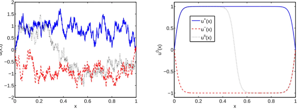
Figure 2. (Top) Shown are three sample solutions to (18), the discretized version of (2), with Dirichlet boundary conditions, at various instances in time, with potential function (20), N = 1024 discretization points, δ = 0.03, and initial conditions with energy N/β and β∆E = 4.6. The blue solid line is a solution near the minimizer u+(x), the red dashed line is a solution near the minimizer u−(x) and the black dotted line is in the process of transitioning
from u+(x) to u−(x). (Bottom) These critical points along with one of the
saddles, us(x), separating them.
are chosen approximately from the invariant measure (6) with the double well potential (20) and Dirichlet boundary conditions.
McKean and Vaninsky [20] (see also [14, 33]) verified that (6) is an invariant measure of (2) with periodic boundary conditionsu(0, t) = u(1, t). This invariance of the Gibbs measure is not unique to the wave equation and has been shown for other Hamiltonian PDEs such as the nonlinear Schr¨odinger equation [4, 18, 28, 29], Korteweg-de Vries equation [23], and others [22, 9].
We have added to (6) the parameterβnot present in McKean’s original results. Consistent with the aforementioned scaling of the variance of the stochastic functions p(x) andu(x) by 1/β, the parameter β, added to the measure (6), is playing the roll of an inverse tempera-ture. Recall the measure (6) is also an invariant measure for the noisy-damped system (5) regardless of the value of γ >0, the damping parameter. In this case, the temperature β−1
characterizes the size of the fluctuations driving the system, and therefore the variance of the solutions. In terms of the system with Hamiltonian (3), the parameter β−1 acts like a
temperature parameter and also characterizes the spatial variance of the weak solutions.
4. Expected Residency Times from Transition State Theory
with initial distribution given by the invariant measure (6). We start by considering the finite dimensional system (18), with initial conditions selected from the invariant measure (23), and then justify the infinite dimensional limit. The same calculation for the microcanonical invariant measure (21) is considered in appendix C.
4.1. TST Revisited in an Averaged Set-up. For a Hamiltonian system, we follow a similar derivation to those in [30, 27] but do not assume ergodicity at this point. We divide the finite dimensional phase space, u,p∈ RN into two regions, B− containing (0,u−) and B+ containing (0,u+), by mean of a dividing surface S that separates the two: how to
specify this surface will be discussed later in Sec. 4.2. For a single trajectory, the average TST frequency of transitions from region B− to B+ over a time T >0 is given by
(31) νST(u(0),p(0)) = 1
TNT(u(0),p(0))
whereNT(u(0),p(0)) counts the number of times the trajectoryu(t) solution of (18) for the
initial condition (u(0),p(0)) leaves the regionB−by crossingSwithin the time interval [0, T]. It is convenient to parametrize S by the zero level set of some function q(u), specifically, (32) S ={(p,u) :q(u) = 0}.
We will explain the specific choice of q(u) leading to the surface in (9) in the next section. For convention, take B+ = {(p,u) : q(u) > 0} and B− ={(p,u) : q(u)< 0}. Transitions
from B− to B+ are then changes in the sign of q(u) from negative to positive. This allows
the frequency to be written as
(33) νST(u(0),p(0)) = 1 T
Z T
0
max
d dtΘ
q(u(t)),0
dt
where Θ(z) is the Heaviside function, Θ(z) = 0 if z <0, Θ(0) = 12, Θ(z) = 1 ifz >0. Using the property that Θ′(z) =δ(z), where δ(z) is the Dirac distribution, using the chain rule to
get to ˙u(t)· ∇q(u(t))δ(q(u(t))), and setting ˙u(t) =p(t), we arrive at
(34) νST(u(0),p(0)) = 1 T
Z T
0
max (p(t)· ∇q(u(t)),0)δ(q(u(t)))dt.
We now want to compute the average ofνT
S over trajectories with initial conditions chosen
with respect to an invariant measure, specifically the canonical distribution (23). By defini-tion, if we denote by (p(t,p0,u0),u(t,p0,u0)) the solution to (18) for the initial condition
(p(0,p0,u0),u(0,p0,u0)) = (p0,u0), for any suitable test function f(p0, u0), we have
(35)
Z
f(p(t,p0,u0),u(t,p0,u0))dMN(p0,u0) = Z
f(p,u)dMN(p,u).
As a result the ensemble average of the integrand in (34) is invariant in time, and after proper interpretation of integration with respect to the Dirac distribution, we arrive at the following expression for the mean frequency
(36) νSc =CN−1
Z
S
max (p·n(ˆ u),0)e−βHN(u,p)d˜σ(p,u)
4.2. Optimal TST. To understand metastability, we are interested in evaluating (36) for the dividing surface S that best separates the two metastable states containing u− and u+, minimizing the mean frequency of transition [30] (and thereby maximizing the transition time). While we may not be able to determine this surface exactly, a reasonable surface to use is the finite dimensional approximation of the codimension one hyperplane given by (4). The hyperplane in (4) passes through the saddle point, perpendicular to the unstable direction of the gradient flow wt(x, t) = δ2wxx(x, t)−V′(w(x, t)). While this surface may
not be the true surface that maximizes the mean transition time, for large β we expect this surface to have minimal re-crossings, and therefore produce a close bound on the mean transition time.
The reasoning for this surface having minimal re-crossings starts with the assumption that most transitions will occur near the saddle point, the lowest energy point on the dividing surface [1]. Near the saddle point, the linearized Hamiltonian system has one hyperbolic direction corresponding to the one unstable direction of the gradient flow; the remaining directions are oscillatory. Any surface not perpendicular to the unstable direction of the gradient flow (which bisects the stable and unstable hyperbolic directions) would also not be orthogonal to all the oscillatory directions of the Hamiltonian flow, allowing for many recrossings of the surface in at least one of the oscillatory directions.
The finite dimensional approximation to (4) is the hyperplane (37) S ={(p,u) : (u−us)·φ(1) = 0}
where us and φ(1) are the discrete equivalents to us and φs, that is: us is the Morse index
1 critical point of
(38) UN(u) =
1 N
N X
j=1
V(uj) +N N X
j=0 1 2δ
2(u
j+1−uj)2,
with minimum energy, and φ(1) is the unique eigenvector with negative eigenvalue of the Hessian of (38) evaluated atu =us. In other words, these vectors solve
0 =δ2N2(usj−1−2ujs+usj+1)−V′(usj) (39)
λskφ(k)j =−δ2N2(φ(k)j−1−2φ(k)j +φ(k)j+1) +V′′(usj)φ(k)j , (40)
when k = 1 and λs
1 < 0 for j = 1, . . . , N and appropriate boundary conditions fixing us0,
us N+1, φ
(k)
0 , and φ (k)
N+1. Note the remaining eigenvectors for k = 2. . . N solve (40) when
λs k >0.
For the canonical measure, (23), intuitively one would expect the measure to concentrate around the points (0,u±) that minimize the Hamiltonian as β → ∞. It is convenient to write an expansion for u in the rotated and rescaled eigenvector basis as
(41) u=u±+ ˜u=u±+
N X
k=1
b±kψ(k)±,
in which the eigenvalues λ±k and the corresponding eigenvectors ψ(k) for each k = 1. . . N solve
(42) λ±kψj(k)±=−δ2N2(ψ(k)j−1±−2ψ(k)j ±+ψj+1(k)±) +V′′(u±j )ψj(k)±
forj = 1. . . N and appropriate boundary conditions fixingψ(k)0 ±andψN(k)+1±. The eigenvectors are normalized to satisfy N1 PN
j=1(ψ (k)±
j )2 = 1, the discrete version of L2 normalization. We
use the same numbering convention as before, λ±j < λ±k if j < k, but this time all the λ±k >0 for k = 1. . . N. The quadratic expansion of the potential energy (38) is
(43)
UN(u)∼UN(u±) +
1 2N
N X
k=1
λ±
k(b±k)2ψ
(k)±·ψ(k)± as u→u±
=EN±+1 2
N X
k=1
λ±k(b±k)2.
Defining ˜pj = ˙b±j , the rotated momenta, the quadratic approximation of the Hamiltonian is
(44) HN ∼EN±+
N X
j=1
1 2Np˜
2 j +
1 2λ
±
j(b±j )2
asu →u±,
where we have defined EN± = UN(u±). We show in appendix B.1 the canonical measure
concentrates into a localized region around the point b± = 0, even as N → ∞ in the following proposition:
Proposition 2. Consider the marginal canonical measure with the quadratic Hamiltonian approximation (44) and an N-dimensional box with side edge lengths 2δj,
DNδ ={b± :−δj ≤b±j ≤δj ∀ j = 1. . . N},
whereδj are such thatPNj=1δj2 converges asN → ∞. Assume that the eigenvaluesλ±j solving
(42) satisfy
λ±j ∼Cj2 as j → ∞, for some C >0
Then, for every δ >ˆ 0, there exists β1 > 0 and a set of {δj}Nj=1 such that for every β > β1
and every N >0
(45)
R DN
δ exp
−β2
PN
j=1λ±j (b±j )2
db±
R
RNexp
−β2
PN
j=1λ±j (b±j)2
db±
>1−δˆ
B+ = {(p,u) : (u− us)· φ(1) > 0} and B− = {(p,u) : (u −us)·φ(1) < 0} that
par-tition space, separated by S,
(46) CN =CN++CN−
where
(47) CN±=
Z
B±
e−βHN(p,u)dpdu.
Now, each region contains only one minimizer of the potential energy. Within region B+,
we expect most of the measure is near u+ while in B−, its in the vicinity ofu−. The result after completing the integration appears below in Proposition 3.
For the integral in (36), the measure is restricted to the surfaceS defined in (37). On this surface, it is the point (0,us) that minimizes the Hamiltonian. We expand about this point, and rotate to an eigenvector basis
(48) u=us+ ˜u=us+
N X
k=1
akφ(k)
with λs
k and φ(k) for each k= 1. . . N solving the system in (40) with appropriate boundary
conditions fixing φ(k)0 , and φ(k)N+1, and normalized to satisfy 1 N
PN
j=1(φ (k)
j )2 = 1. Our
conven-tion is to order the eigenvalues such that λs
1 is the sole negative eigenvalue and λsj < λsk for
j < k. The quadratic approximation of the potential energy (38) is
(49)
UN(u)∼UN(us) +
1 2N
N X
k=1
λska2kφ(k)·φ(k) as u→us
=ENs +1 2
N X
k=1
λska2k
due to the defined normalization of the eigenvectors, and where we have defined Es
N =
UN(us). Defining ˜pj = ˙aj, the rotated momenta, the approximation of the Hamiltonian in
the vicinity of us is
(50) HN ∼ENs +
N X
j=1
1 2Np˜
2 j +
1 2λ
s ja2j
asu→us.
In appendix B.1 we state Proposition 4, an analogous Proposition to 2, for the concentration of the measure restricted to the surface S. This allows the use of (50) to complete the integration in (36).
The following proposition states the asymptotic inβ values of the integrals needed to com-pute the TST frequency in (36). The justification of these formulas appear in appendix B.2.
Proposition 3. For the canonical ensemble, the asymptotic in β → ∞, valid for all N >0, expansion of the integral in (36) is
(51)
Z
S
max (p·n(ˆ u),0)e−βHN(u,p)d˜σ(p,u)∼ 2
N−2NN(N −2)!S 2N−3
βNQN j=2
p
λs j
and the expansion of the integrals in (47) are
(52) CN± ∼ 2
N−1NN(N −1)!S 2N−1
βNQN j=1
q
λ±j
e−βEN±.
In the above, the eigenvalues λs
j, j = 2. . . N solve (40), the eigenvalues λ±j, solve (42) and
Sn = 2π(n+1)/2/Γ((n+ 1)/2) is the surface area of the n-dimensional sphere (embedded in
n+ 1 dimensional space) of unit radius.
Using the above asymptotic in β expansions, the TST frequency from (36) is
(53) νSc ∼ 1
2π
QN
j=2 1 √λs
j
e−βEs N
QN
j=1 q1 λ+
j
e−βEN+ +QN j=1q1
λ−j e
−βE−N.
4.4. Mean Residency Times. The mean residency times on either side of S, given by (37), can be computed with the same integrals considered above. Namely,
(54) τ±c = C
±
N
CNνSc
for the canonical ensemble. With the asymptotic expansions of the integrals in Proposition 3, we arrive at the asymptotic in β expressions for the mean residency time
(55) τ±c ∼2π
QN
j=2 p
λs j
QN
j=1 q
λ±
j
eβ(ENs−E±N).
This expression is valid for all N allowing us to take the limit as N → ∞, arriving at τ± in (14), provided the infinite product Λ± give in (15) converges. It is the infinite dimensional limit of the finite dimensional eigenvalue products in (55). For example, Λ± converges when considering eigenvalues related to the Laplacian in one spatial dimension, as we do here (however it does not for two or more spatial dimensions).
5. Numerical Results
Using numerical simulations of the finite dimensional truncation of (2), we investigate the implication of our results for the long time dynamics of the nonlinear wave equation. We proceed in two steps. First, we validate our approximations by considering an ensemble of trajectories chosen approximately from the finite dimensional truncation of the invariant measure (6), and estimating numerically the mean residency time averaged over these initial conditions. Second, we compute the residency time averaged over a single trajectory in order to investigate the extent to which the dynamics of (2) is ergodic and mixing with respect to the invariant measure (6). We find support for this statement for small values of the exchange coupling δ. For larger values of δ, however, we observe that either ergodicity fails, or the mixing time grows so much that we cannot observe convergence of the time averages towards their ensemble counterparts averaged over the invariant measure (6).
for the Hamiltonian (44). Specifically, p∈RN is a discretization of white noise andu∈RN
is a Gaussian random variable with known mean and covariance. They are computed as
(56) p=
s
N
β h, u=u
++ α
√
β
N X
j=1
gj q
λ+jψ(k)+
in which h= (h1, . . . hN) andg = (g1, . . . gN) are vectors ofN independent mean zero
stan-dard Gaussian random variables, u+= 1 for Neumann boundary conditions, the eigenvalues λ+ and eigenvectors ψ(k)+ solve (42), normalized such that ψ(k)+ ·ψ(k)+ = N, and α is
chosen to ensure the energy of the initial condition isN/β exactly.
For the potential function (20), the system is symmetric. We therefore determine the mean transition time by taking the total simulation time and divide it by the number of transitions across the diving hyperplane S described in section 4.2. Specifically, we compute the eigenvector ψ(1) solving (40), the normal vector to the surface S. At each time step, we compute the distance to this dividing surface. A change in sign of the distance indicates a crossing of the surface. Notice that for δ < 1/π there are two saddle points, yet they both lie in the just described plane.
In Fig. 3 (a) we show excellent agreement between the mean transition time found from the numerical simulations at finite N = 128 averaged over an ensemble of 1000 trajectories, and the infinite dimensional theory, (14). We choose two values of δ, one smaller than the bifurcation point δ= 1/π in whichus is non-uniform and one larger than this point in which
case us = 0. This agreement supports the validity of the quadratic approximation used in
obtaining (14).
Next we investigate the ability of the TST time to describe the mean transition time of a single trajectory. As we pointed out above in the derivation of τ±, we would arrive at the same expression had we assumed the flow was ergodic with respect to the invariant measure. Recall in finite dimensions, no Hamiltonian systems are ergodic with respect to the invariant measure given by the canonical ensemble while many are conjectured to be ergodic with respect to the invariant measure given by the micro-canonical ensemble [26]. In infinite dimensions, McKean and Vaninsky conjectured that the flow of (2) is ergodic (a.k.a. metrically transitive) with respect to the measure (6) except for completely integrable systems with an infinite number of conserved quantities like V′(u) =u,sinu or sinh u [20].
Although the measure (6) looks like the canonical distribution, we argued its equivalence to the microcanonical measure, and therefore do not find an assumption of ergodicity surprising. Indeed, at small values of δ, we find numerical evidence for ergodicity, and agreement between the mean transition time found from a long-time average over a single trajectory and the time (14) as shown in Fig. 3(b). In this semi-log plot, the slope of the lines are∆E+
(for Neumann boundary conditions this is solelyEs, the value of which is show in Fig. 1 as a
function ofδ), while the y-intercept is given by the prefactor, 2πΛ+. The eigenvalue produce
Λ+ is shown in Fig. 3(c) as a function ofδ, computed with a truncation of N = 1024.
β
0 10 20 30 40
log(
τ
)
0 1 2 3 4 5 6 7 8 9 10
(a)
δ = 0.2
δ = 1.
β
0 500 1000 1500 2000 2500
log(
τ
)
0 1 2 3 4 5 6 7 8 9 10
(b)
δ = 0.03
δ = 0.01
δ=0.003
δ
0 0.5 1 1.5 2
Λ+
0 5 10 15 20 25
(c)
Figure 3. (a) Log of the mean transition time as a function ofβ(symbols) av-eraged over an ensemble of 1000 trajectories chosen according to (56), evolved by numerically simulating (18), with potential function (20) andN = 128 and (lines) the theoretical value of τ+ given by (14). (b) Log of the mean
transi-tion time (symbols) computed from a long time average of a single trajectory chosen according to (56) and (lines) the theoretical value of τ+ given by (14).
(c) The prefactor Λ+ in (15) computed numerically with N = 1024 points as
a function of δ. As the bifurcation point δ = 1/π is approached, the prefactor goes to zero because one of the eigenvalues of the saddle point is about to cross zero.
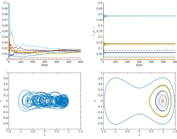
This loss of ergodicity can be explained by a fundamental change in the dynamics as δ increases. Not only does increasingδreduce the size of the fluctuations in the solutionu(x, t), but it also makes this solution more uniform in x. This is evident from the energy penalty proportional to δ2 on the x-derivatives in the Hamiltonian (3), which also lead to the loss
of the non-trivial saddle point for δ > 1/π. The solutions to (2) at each instance in time become approximated by small fluctuations in space about the quantity ¯u(t) =R1
0 u(x, t)dx.
These effects can be quantified by starting from a largeβ expansion foru(x, t), the infinite dimensional version of what was presented in Sec. 4.3. Taking
(57) u(x, t) =u+(x) + √1
time
0 100 200 300 400 500 600
<
¯
p
2
>
0 0.01 0.02 0.03 0.04 0.05 0.06 0.07 0.08 0.09 0.1
time
0 100 200 300 400 500 600
<
¯
p
2
>
0 0.05 0.1 0.15 0.2 0.25 0.3 0.35 0.4 0.45 0.5
¯ u
-1.5 -1 -0.5 0 0.5 1 1.5
¯
p
-1 -0.8 -0.6 -0.4 -0.2 0 0.2 0.4 0.6 0.8 1
¯ u
-1.5 -1 -0.5 0 0.5 1 1.5
¯
p
-1 -0.8 -0.6 -0.4 -0.2 0 0.2 0.4 0.6 0.8 1
Figure 4. Results of numerical simulations of the finite dimensional system (18) with N = 1024. Simulations starting from 9 different initial conditions, selected according to (56), with β∆E = 3, (left) δ = 0.05 (right) δ = 1, were run until t = 600 (much larger than the mean transition time). (top) To emphasize ergodicity in the case of small δ, the time-averaged value of ¯
p2 = PN
j=1p2j/N is plotted, and its value of 1/β obtained from averaging
over the invariant measure (6) is shown as a dotted line. (bottom) Dynamics of the same numerical simulations plotted in terms of the reduced variables ¯
u=PN
j=1u2j/N and ¯p=
PN
j=1pj/N. (bottom left) Single trajectory, (bottom
right) all 9 trajectories.
and expanding the Hamiltonian to quadratic order in β−1/2, the resulting canonical
distri-bution describes ˜uas a Gaussian process with covariance function
(58) C(x, y) =
ex/δ+e−x/δ
e(1−y)/δ +e−(1−y)/δ
2δ e1/δ−e−1/δ x≤y
ey/δ+e−y/δ
e(1−x)/δ+e−(1−x)/δ
2δ e1/δ−e−1/δ x≥y
,
derived in appendix A.2. The uniformity of ˜u(x) inx is apparent from the δ−1 exponential
Gaussian random variables, gn,
(59) u(x)≈ ±1 + √1
β
"
g0+
∞ X
n=1
cos(nπx)
√
1 +δ2n2π2gn #
in which cos(nπx) and 1/(1+δ2n2π2) forn= 0,1,2. . . are the eigenfunctions and eigenvalues
of the covariance C(x, y) in (58). For small δ, a number of the n ≥ 1 terms are significant, while for large δ we see that only the constant zeroth order term is significant.
Another way to interpret this largeδ behavior is that only the first constant mode of the solution contributes significantly to the dynamics, namely
¯ u(t) =
Z 1
0
u(x, t)dx and p(t) =¯
Z 1
0
p(x, t)dx.
The dynamics of these reduced variables are shown in the bottom row of Fig. 4. For small δ in the bottom left plot, a solution trajectory explores the phase-space, while for large δ in the bottom right plot, each trajectory with a different randomly chosen initial condition appears to neraly conserve the reduced Hamiltonian,
¯ H = 1
2p¯
2+V(¯u),
violating the assumption of ergodicity with respect to the canonical measure with the original Hamiltonian. The conservation of the reduced Hamiltonian in the limit of large δ can be understood by computing the time evolution of the quantity. Namely,
dH¯ dt = ¯p
Z 1
0
dp
dtdx+V
′(¯u)
Z 1
0
du dtdx
= ¯p
Z 1
0
(δ2uxx−V′(u))dx+V′(¯u)¯p=O(δ−1)
in which the last equality holds since R1 0 δ
2u
xxdx= 0 by the Neumann boundary conditions,
and V′(u) = V′(¯u) +O(δ−1) when u(x) is nearly uniform by the expansion in (59).
6. Conclusions
We have investigated the dynamics of the nonlinear wave equation (1), with particular interest in metastability and mean transition times. We discussed how the finite dimen-sional microcanonical distribution, with energy scaling extrinsically as N/β, is equivalent to the canonical distribution as N → ∞. By revisiting transition state theory (TST) for an ensemble of trajectories chosen with the canonical invariant measure of the finite dimen-sional Hamiltonian system, we derived the mean frequency at which the solutions cross a dividing surface separating the two minimizers of the Hamiltonian. Extension to the PDE case required we justify the use of a quadratic approximation of the Hamiltonian in infinite dimensions by showing concentration of the canonical invariant measure for arbitrarily large N. Numerical simulations of the finite dimensional Hamiltonian system supported that the TST time applied for almost all initial conditions only if δ was small.
values of δ, the mixing time appears to be much shorter than the computed mean residency time with TST, suggesting that the metastable dynamics could be approximately coarse-grained onto that of a two-state Markov jump process for the two localized regions around the minimizers. At intermediate values of δ, the increase in the mixing time causes correlations between successive transitions. Even though the system could still be ergodic with respect to the canonical invariant measure, the time to observe convergence of long-time averages increases. In fact, the results in Sec. 5 suggest that this mixing time goes to infinity at least as O(δ1) as δ → ∞ and, in particular, eventually becomes much bigger than the residency
times in the metastable sets.
The simulated dynamics of the deterministic nonlinear wave equation also provides in-teresting insight into the low-damping, γ → 0, regime of the Langevin equation (5). The mean transition time computed with large deviation theory (LDT) in (17) is equivalent to the TST time (14) in the limit as γ → 0. The implied equivalence of trajectory-wise dy-namics is supported only by the numerical simulations of the deterministic system in the small δ regime, in which the mean transition time computed over a single trajectory is well described by the TST time. In this regime, both the deterministic equation (2) and its stochastic counterpart (5) have equivalent transition times.
This is in contrast to the large δ regime in which the numerical simulations of the de-terministic equation effectively behave like those of a one-dimensional Hamiltonian system, approximately conserving a reduced energy. This illuminates what we might expect from the low-damping regime of the Langevin equation (5). It should behave like a one-dimensional noisy-damped system, with values of reduced energy that are often less than the value of the saddle point energy and slowly diffusing relative to the timescale of a typical Hamiltonian or-bit. We would therefore expect the method of averaging [13], applied to the reduced variables rather than the full system, to characterize the motion of the reduced energy. Computing the transition times for the reduced energy as we did in [21] would produce a prefactor, inversely proportional to the damping, on the exponential transition time that is much larger than the lower bound computed here with TST. We hope to pursue this further in future work.
We end with a final remark that the derivation of the TST time cannot be extended to the wave equation in multiple (D≥2) spatial dimensions. While the system can still be dis-cretized to form a finite dimensional system, the limit towards the continuous system breaks down. We cannot justify metastability through the concentration of the invariant measure, and the prefactor containing the eigenvalues in (14) fails to converge. These problems, stem-ming from the eigenvalues of the Laplacian in multiple spatial dimensions, are reminiscent of known problems with solutions to stochastic partial differential equations like (5) when D≥2 [15, 25].
acknowledgements. We would like to thank Weinan E and Gregor Kovaˇciˇc for useful discussions. This work was supported in part by the NSF grant DMS-1522767 (E. V.-E.).
Appendix A. Infinite Dimensional Microcanonical Distribution
In this appendix, we prove proposition 1. We show the limit of the microcanonical distri-bution as N → ∞, with energy given by EN =N/β, leads to the invariant measure written
formally in (6) by calculating the characteristic function of bothu(x, t) andp(x, t) =ut(x, t).
We do this exactly for a quadratic Hamiltonian, with V(u(x)) = 1 2f(x)u
2(x), and explicitly
We begin with the discrete microcanonical distribution (21) with energy EN for a finite
dimensional quadratic Hamiltonian,
(60) dµN =c−N1δ
EN −
1 2Np
Tp
− 12uTANu
dpdu
where the N ×N matrix AN is such that uTANu = N1 Pj=0N δ2N2(uj+1−uj)2 +f(xj)u2j
with u0 and uN+1 set by the boundary conditions of (1). As N → ∞ we have uTANu → R1
0 u(x) − δ
2 d2
dx2 +f(x)
u(x)dx. Note the matrix AN is symmetric in the case of either
Dirichlet or Neumann boundary conditions.
We consider the characteristic function for the {uj} first, finding it converges to
(61) φu(t)→exp
− 1
2β
Z 1
0
Z 1
0
t(x)C(x, y)t(y)dxdy
,
a Gaussian process with covarianceC(x, y)/β. The covariance function is obtained by solving
δ2 d
2
dx2 +f(x)
C(x, y) =δ(x−y)
with appropriate boundary conditions. A few special cases are given in Sec. A.2. Then we follow a similar procedure for the {pj} in Sec. A.3, finding the characteristic function
converges to
(62) φp(s)→exp
− 1
2β
Z 1
0
s(x)2dx
,
a Gaussian process with covariance δ(x−y)/β (i.e. white noise). These are combined to arrive at proposition 1.
A.1. The u. The characteristic function for the sets of points u selected from the micro-canonical distribution (60) is defined as
(63) φu(t) = Z
R2N
eNitTuδ
EN −
1 2Np
Tp
−12uTANu
dpdu
Z
R2N
δ
EN −
1 2Np
Tp
− 12uTANu
dpdu
.
The integral in the denominator of (63) is determined first by switching to the coordinates
q=A1/2N u and rescaling pto be p/√N. This results in the integral NN/2
detA1/2N
Z
R2N
δ
EN −
1 2p
Tp
− 1
2q
Tq
dpdq
where detA1/2N =QN j=1
p
λj and theλjare the eigenvalues of the matrixAN. Then, switching
to spherical coordinates, r2 =PN
j=1p2j, we have
NN/2
detA1/2N SN−1
Z
RN
Z ∞
0
δ
EN −
1 2q
Tq− r2
2
where SN−1 =NπN/2/Γ(N/2 + 1) is the surface area of the sphere inN-dimensional space,
and integrating over r we obtain NN/2
detA1/2N SN−1
Z
RN
EN −
1 2q
Tq
N/2−1
+
dq,
where x+= max(0, x). Last, we switch to spherical coordinates for the q,
NN/2
detA1/2N (SN−1)
2
Z √2EN
0
EN −
r2
2
N/2−1
rN−1dr
which is equivalent to
(64) N
N/2
detA1/2N (SN−1)
2EN−1 N
√
π Γ(N/2) 2N/2Γ(N/2 + 1/2).
For the numerator of (63) we again switch to the coordinates q = A1/2N u and rescale the
p top/√N, obtaining NN/2
detA1/2N
Z
R2N
eNitTA
−1/2
N qδ
EN −
1 2p
Tp
− 12qTq
dpdq.
Switching the pto spherical coordinates and integrating yields NN/2
detA1/2N SN−1
Z
RN
eNitTA
−1/2
N q
EN −
1 2q
Tq
N/2−1
+
dq.
To determine the integral over q, we write the integral in spherical coordinates over all ˆ
n∈Ω, the unit normal to the N-dimensional sphere, and allr,
(65) N
N/2
detA1/2N SN−1
Z √2EN
0
Z
Ω
eNitTA
−1/2
N nˆr
EN −
r2
2
N/2−1
rN−1dnˆdr.
The appearance of the ˆn in the exponent does not allow us to integrate exactly. Before proceeding, we return to our original expression (63) by taking the ratio of (65) to (64), resulting in
(66) φu(t) =
2N/2Γ(N/2 + 1/2)
ENN−1√πΓ(N/2) 1 SN−1
Z √2EN
0
Z
Ω
eNitTA 1/2 N nˆr
EN −
r2
2
N/2−1
rN−1dnˆdr.
In (66), the integral over ˆndivided by the surface area can be thought of as an expectation with respect to the random variable ˆn, the unit vector chosen uniformly over the surface of the unit sphere in N-dimensional space,
1 SN−1
Z
Ω
eNitTA 1/2
N nˆrdnˆ =E h
eNitTA
−1/2
N nˆr i
.
Alternatively, we can express the random variable ˆn as g/|g| where g is an N-dimensional vector with components that are independent identically distributed mean zero Gaussian random variables. Intuitively, for large N this random variable can be approximated by
g/√N (noticed by Poincar´e [24], see also [19]). More specifically, in the limit as N → ∞we have that the expectation over ˆn scales as
E exp i Nt T
A−N1/2nˆr
∼E exp i N3/2t
T
A−N1/2gr
where we use ∼ to indicate that the ratio of the two sides approaches one asN → ∞. This expectation on the right hand side is the characteristic function of a mean zero multivariate Gaussian; it is known explicitly. Combining the above results we have
(67) 1
SN Z
Ω
eNitTA 1/2
N nˆrdnˆ ∼exp
−1
2 r2
N3t TA−1
N t
in the limit of large N.
Then, inserting (67) into (66) for the integration over ˆn we are left with the following integral,
(68)
Z √2EN
0
e−12 r2 N3tTA−
1 N t
EN −
r2
2
N/2−1
rN−1dr.
We would like to use Laplace’s method,
Z b
a
g(x)eN f(x)dx∼
s
2π
N|f′′(x0)|g(x0)e
N f(x0)
if the integral in (68) has the proper scalings as N → ∞. We notice the scaling of the exponent in (68) is r2/N +O(1) astTA−1
N t/N2 converges to a double integral,
1 N2t
TA−1 N t→
Z 1
0
Z 1
0
t(x)C(x, y)t(y)dxdy
where the function C(x, y) is obtained by inverting the operator A∞, defined such that
uTANu → R1
0 u(x)A∞(x)u(x)dx. This exponential term in (68) remains smaller than e N as
N → ∞ provided the maximum value ofr does not grow faster thanO(√N). The exponential in N component comes from writing
EN −
r2
2
N/2−1
rN−1 ∼exp
N
2 log(EN − r2
2) +Nlogr
to leading order in N. We see that this exponent attains its maximum between r = 0 and
√
2EN when r =√EN. This corresponds to half of the total energy, EN, contained within
the variables u; the equipartition of energy between the p and theu.
Now, we define the value of the energy,EN =N/β, as this is where the canonical measure
energy concentrates, as discussed in the main text. Even with this energy scaling with N, and therefore the maximum value of r = pN/β, the exponential term in (68) remains smaller thaneN. Applying Laplace’s method to the integral in (68), with energyE
N =N/β,
we obtain
Z √2N/β
0
e−12 r2 N3tTA−
1 N t N β − r2 2
N/2−1
rN−1dr
∼
N β
N−1
2−N/2+1
r
2π N4exp
−1
2 1 βN2t
TA−1 N t
asN → ∞. Combining this result together with (67) into (66) also withEN =N/β, we find
after simplifying that
φu(t)∼
Γ(N/2 + 1/2) Γ(N/2)
r
2 N exp
−2β1 N12t T
A−N1t
In the limit as N → ∞ the prefactor in this expression goes to unity (the true value of the integral of (1−r2/2)N/2−1rN−1 and its approximation are asymptotically equivalent), leaving
(69) φu(t)→exp
−2β1
Z 1
0
Z 1
0
t(x)C(x, y)t(y)dxdy
.
The stochastic process u(x) has the covariance function C(x, y)/β. The covariance function C(x, y) is found by solving
(70) A∞C(x, y) = δ(x−y)
with appropriate boundary conditions. We consider special cases of A∞ in the next section before proceeding to consider the characteristic function of the p.
A.2. Example Covariance Functions. Analytic solutions to (70) can be obtained in a few special cases. Of particular interest is the case of the quadratic function V(u) = 1
2u 2,
which can be used to approximate the nonlinear potential function V(u) = 14(1−u2)2 near
its minimizers.
For the case of dynamics governed by (2) withV(u) = 1 2u
2 and Dirichlet boundary
condi-tions, u(0, t) =u(1, t) = 0, inverting the operator A∞ amounts to solving
(71)
−δ2 ∂
2
∂x2 + 1
C(x, y) =δ(x−y)
with boundary conditions C(0, y) = C(1, y) = 0 and continuity conditions at x = y. The solution is
(72) C(x, y) =
ex/δ−e−x/δ
e(1−y)/δ −e−(1−y)/δ
2δ e1/δ−e−1/δ x≤y
ey/δ−e−y/δ
e(1−x)/δ−e−(1−x)/δ
2δ e1/δ−e−1/δ x≥y
This covariance is nearly constant along a large portion ofx=y, indicating the solutions look something like an Ornstein Uhlenbeck process, but conditioned to have u(0, t) =u(1, t) = 0. When the boundary conditions are changed to Neumann boundary conditions, the solution to (71) is
(73) C(x, y) =
ex/δ+e−x/δ
e(1−y)/δ +e−(1−y)/δ
2δ e1/δ−e−1/δ x≤y
ey/δ+e−y/δ
e(1−x)/δ+e−(1−x)/δ
2δ e1/δ−e−1/δ x≥y
To understand what these covariance functions describe, consider no potential function, V(u) = 0, and Dirichlet boundary conditions. The covariance is given by the solution to
−δ2 ∂
2
∂x2C(x, y) = δ(x−y)
with boundary conditions C(0, y) =C(1, y) = 0, which is
(74) C(x, y) = min(x, y)−xy δ2 ,
A.3. Thep. We can follow the exact same procedure to compute the characteristic function for the p,
(75) φp(s) = Z
eNisTpδ
EN −
1 2Np
Tp− 1
2u
TA Nu
dpdu
Z
δ
EN −
1 2Np
Tp
− 12uTANu
dpdu
.
Much of the above derivation follows directly, and we briefly detail the steps. By rescaling
p to bep/√N and q =A1/2N u we have
φp(s) = Z
e√iNs Tp
δ
EN −
1 2p
Tp
− 12qTq
dpdq
Z
δ
EN −
1 2p
Tp
− 12qTq
dpdq
.
switching to spherical coordinates and replacing ˆnwith the scalingg/√N within the expec-tation results in
φp(s) =
Z √2EN
0 E
h
e√iNs Tgri
EN −
r2
2
N/2−1
+
rN−1dr
Z √2EN
0
EN −
r2
2
N/2−1
+
rN−1dr
.
Using that the expectation
E
exp( i Ns
Tgr)
= exp(− r
2
2N2s Ts)
and using Laplace’s method for the integral over r with the scaling of EN =N/β we arrive
at
(76) φp(s)→exp
− 1
2β
Z 1
0
s(x)2dx
in the limit as N → ∞. (Note that 1 Ns
Ts→ R1 0 |s(x)|
2dx). Thus we see that p(x) is white
noise with covariance function δ(x−y)/β.
Appendix B. Quadratic Approximation
B.1. Concentration of the Canonical Measure. In the following, we show the concen-tration of the marginal canonical measure for b± = (b±1, . . . b±N) as stated in Proposition 2 in the main text, and also for the marginal canonical measure restricted to the surface S ={(˜p,a) :a1 = 0}in the eigenvector basis, stated in Proposition 4 below.
We first point out that the constraint onPN
j=1δ2j is to ensure the corner of the box remains
a finite distance away from the center of the box regardless of the value ofN, in particular as N → ∞. Therefore the measure is being contained within a localized region. In particular, the sides of the box must decay faster than 1/√j,
(77) δ2j ∼ C
j1+ǫ,
for some ǫ >0 andC >0.
We drop the ± and proceed to calculate
(78)
R DN
δ e −β2
PN j=1λjb
2 jdb R
RNe− β 2
PN j=1λjb
2 jdb
.
by squaring everything so each integral over bj becomes an integral over bj and aj: Z δj
−δj Z δj
−δj
e−β2(λjb 2
j+λja2j)db jdaj
Z ∞
−∞
Z ∞
−∞
e−β2(λjb 2
j+λja2j)db jdaj
.
Then, rescaling by the eigenvalues and noting the integral over the 2D square with sides 2δj
p
λj is greater than the integral over the circle with radiusδj p
λj, gives
Z δj√λj
−δj√λj
Z δj√λj
−δj√λj
e−β2(b 2 j+a
2 j)db
jdaj
Z ∞
−∞
Z ∞
−∞
e−β2(b 2 j+a2j)db
jdaj
>
Z δj√λj
0
e−β2r 2
rdr
Z ∞
0
e−β2r 2
rdr
=1−e−β2δ 2 jλj
for each j = 1. . . N.
Combining all the integrals, which are identical, we are left with showing that there exists a β1 such that
(79)
N Y
j=1
1−exp
−β2δ2jλj
>(1−δ)ˆ2
can be satisfied for all N >0 and for all β > β1.
The product in (79) converges if the sum
(80)
N X
j=1
log
1−exp
−β2δj2λj
converges as N → ∞. We can compare the decay of the terms in this sum to the decay of the terms in a known converging series, P∞
are negative, so we add a negative sign and compare. We are interested if
(81) lim
j→∞
−log1−e−β2δ 2 jλj
1/jp <∞
Taking the derivative of top and bottom yields
(82) lim
j→∞
jp+1β
2δ2jλje− β 2δ
2 jλj
p1−e−β2δ 2 jλj
= 0,
provided the exponent in the numerator decays to zero,
(83) δ2
jλj → ∞
as j → ∞.
We are left to consider if there exits a box with sides 2δj that satisfies both (77) and (83)
simultaneously. This depends on the values of the λj. For our application, they are the
eigenvalues of the operator (16). They are dominated by the Laplacian term, and therefore for large j scale like
(84) λj ∼j2.
From (77) we have that ǫ > 0 and from combining (77) and (84) into (83) we have that 1−ǫ > 0. A range of values of ǫ are possible, for example, ǫ = 1/2. Thus it is possible to contain the measure within a finite region around a minimizer of the Hamiltonian. With a choose of ǫ, the value of β1 is determined as the one that satisfies (79) when N → ∞ (the
product is decreasing as N increases).
The integration for the TST frequency also requires the following proposition concern-ing the concentration of the measure restricted to the surface S, given by a1 = 0 in the
eigenvector coordinates:
Proposition 4. Consider the marginal canonical measure restricted to the surface S defined in (37) with the quadratic Hamiltonian approximation (50) and an N −1-dimensional box with side edge lengths 2δj,
¯
DNδ−1 ={a:a1 = 0,−δj ≤aj ≤δj ∀ j = 2. . . N},
satisfying PN
j=2δj2 remaining finite as N → ∞. Assume that the eigenvalues λsj solving (40)
satisfy
λs
j ∼Cj2 as j → ∞, for some C >0
Then, for every δ >ˆ 0, there exists β1 > 0 and a set of {δj}Nj=2 such that for every β > β1
and every N >0
(85)
R ¯ DN−1
δ exp
−β2
PN
j=2λsja2j
da2. . . daN
R
RN−1exp
−β2
PN
j=2λsja2j
da2. . . daN
>1−δˆ
The proof of Proposition 4 follows exactly, replacing all summations above from j = 2. . . N. In particular, the expression in (80) becomes
(86)
N X
j=2
log
1−exp
−β2δj2λsj