MODELING OF COMPLEX LARGE-SCALE FLOW PHENOMENA
Abhinav Golas
A dissertation submitted to the faculty of the University of North Carolina at Chapel Hill in partial fulfillment of the requirements for the degree of Doctor of Philosophy in the
Department of Computer Science.
Chapel Hill 2015
Approved by:
Ming C. Lin
Dinesh Manocha
David Adalsteinsson
Anselmo Lastra
ABSTRACT
Abhinav Golas: MODELING OF COMPLEX LARGE-SCALE FLOW PHENOMENA.
(Under the direction of Ming C. Lin)
Flows at large scales are capable of unmatched complexity. At large spatial scales, they
can exhibit phenomena like waves, tornadoes, and a screaming concert audience; at high
den-sities, they can create shockwaves, and can cause stampedes. Though strides have been made
in simulating flows like fluids and crowds, extending these algorithms with scale poses
chal-lenges in ensuring accuracy while maintaining computational efficiency. In this dissertation,
I present novel techniques to simulate large-scale flows using coupled Eulerian-Lagrangian models that employ a combination of discretized grids and dynamic particle-based
represen-tations. I demonstrate how such models can efficiently simulate flows at large-scales, while
maintaining fine-scale features.
In fluid simulation, a long-standing problem has been the simulation of large-scale scenes
without compromising fine-scale features. Though approximate multi-scale models exist,
accurate simulation of large-scale fluid flow has remained constrained by memory and
com-putational limits of current generation PCs. I propose a hybrid domain-decomposition model
that, by coupling Lagrangian vortex-based methods with Eulerian velocity-based methods,
reduces memory requirements and improves performance on parallel architectures. The
re-sulting technique can efficiently simulate scenes significantly larger than those possible with
either model alone.
The motion of crowds is another class of flows that exhibits novel complexities with
in-creasing scale. Navigation of crowds in virtual worlds is traditionally guided by a static global
cap-ture long-range crowd interactions commonly observed in pedestrians. This discrepancy can
cause sharp changes in agent trajectories, and sub-optimal navigation. I present a technique
to add long-range vision to virtual crowds by performing collision avoidance at multiple
spa-tial and temporal scales for both Eulerian and Lagrangian crowd navigation models, and a
novel technique to blend both approaches in order to obtain collision-free velocities efficiently.
The resulting simulated crowds show better correspondence with real-world pedestrians in
both qualitative and quantitative metrics, while adding a minimal computational overhead.
Another aspect of real-world crowds missing from virtual agents is their behavior at
high densities. Crowds at such scales can often exhibit chaotic behavior commonly known
as crowd turbulence; this phenomenon has the potential to cause mishaps leading to loss of life. I propose modeling inter-personal stress in dense crowds using an Eulerian model,
coupled with a physically-based Lagrangian agent-based model to simulate crowd turbulence.
I demonstrate how such a hybrid model can create virtual crowds whose trajectories show
visual and quantifiable similarities to turbulent crowds in the real world.
The techniques proposed in this thesis demonstrate that hybrid Eulerian-Lagrangian
modeling presents a versatile approach for modeling large-scale flows, such as fluids and
ACKNOWLEDGMENTS
I would like to thank the many people who have made this dissertation possible. First
and foremost, my advisor Ming C. Lin, who has supported my work – both sane and crazy –
throughout my time at UNC, and provided valueable feedback in getting me past roadblocks,
as well as improving my dismal writing skills. I also owe a great debt of gratitude to my
committee members: Dinesh Manocha for opening my mind to new research problems and
directions, Jason Sewall for teaching me how to think about parallel computing, and being
an amazing help during deadlines and otherwise, Anselmo Lastra for showing me a new side
of computer graphics I never knew existed, and David Adalsteinsson for helping me with
math I could never wrap my head around. Without their help and support, this dissertation
would not have been possible.
This dissertation is by no means an individual achievement, and I owe thanks to a lot of
collaborators and coauthors. The biggest thanks of all to Rahul Narain, whose wizardry has
given form to most of my ill-formed ideas. No less helpful have been my other collaborators:
Sean Curtis, Jason Sewall, and Pavel Krajcevski.
I have been lucky to have friends who have served as sounding boards, and who I owe
many thanks: Ravish Mehra, Shabbar Ranapurwala, Riha Vaidya, Gurkaran Buxi, Rachit
Kumar, Stephen Guy, David Wilkie, and Anish Chandak. These are a few of the many
people who have made my time at UNC memorable.
I must point out that this dissertation would not have existed had it not been the constant
prodding of my father to pursue a Ph.D. especially when I had never considered one, my
mother helping me every bit of the way, and my sister and brother for teaching me a good
TABLE OF CONTENTS
LIST OF TABLES . . . x
LIST OF FIGURES . . . xiv
1 Introduction . . . 1
1.1 Modeling Flows . . . 4
1.1.1 Eulerian Representation . . . 5
1.1.2 Lagrangian Representation . . . 7
1.2 Utilizing Parallel Desktop Architectures. . . 8
1.3 Coupled Hybrid Simulation . . . 10
1.4 Thesis Statement . . . 11
1.5 Main Results . . . 11
1.6 Organization . . . 14
2 Large-scale Fluid Simulation using Velocity-Vorticiy Domain Decompo-sition . . . 15
2.1 Introduction . . . 15
2.2 Related Work . . . 17
2.2.1 Velocity-based methods. . . 18
2.2.2 Vorticity-based methods . . . 19
2.3 Hybrid Fluid Simulation . . . 21
2.3.1 Subdomains . . . 22
2.3.2 Hybrid Domain Decomposition . . . 24
2.3.4 Vorticity exchange . . . 27
2.4 Efficient vortex particle simulation . . . 29
2.4.1 Well-conditioned vortex sheet computation . . . 30
2.4.2 Hierarchical methods for flux computation . . . 31
2.5 Results . . . 32
2.5.1 Performance . . . 34
2.5.2 Controlling Dissipation . . . 35
2.6 Summary . . . 35
2.6.1 Limitations and future work . . . 36
3 Hybrid Long-Range Collision Avoidance for Crowd Simulation . . . 39
3.1 Introduction . . . 39
3.2 Background . . . 42
3.3 Lookahead for Long-Range Collision Avoidance . . . 45
3.3.1 Continuum Lookahead . . . 48
3.3.2 Discrete Lookahead . . . 50
3.4 Curtailing Lookahead . . . 52
3.4.1 Obstacles . . . 53
3.4.2 Chaotic Crowds . . . 54
3.5 Hybrid Crowd Simulation . . . 56
3.6 Results . . . 59
3.7 Comparison to Real-World Data . . . 61
3.8 Summary and Future Work . . . 63
4 Simulation of Turbulent Behavior in Human Crowds . . . 75
4.1 Introduction . . . 75
4.3 Continuum Model for Crowd Turbulence . . . 79
4.3.1 Crowd as a Continuum . . . 79
4.3.2 Continuum Turbulence Model . . . 80
4.3.3 Local Collision Avoidance . . . 82
4.4 Inter-personal Stress . . . 83
4.5 Validation . . . 86
4.5.1 Hajj . . . 97
4.5.2 Love Parade 2010 . . . 98
4.5.3 Importance of Friction in Simulating Crowd Turbulence . . . 99
4.6 Summary . . . 99
5 Conclusion . . . 101
5.1 Summary of Results . . . 101
5.2 Limitations . . . 103
5.3 Future Work . . . 104
5.4 Acknowledgments . . . 105
LIST OF TABLES
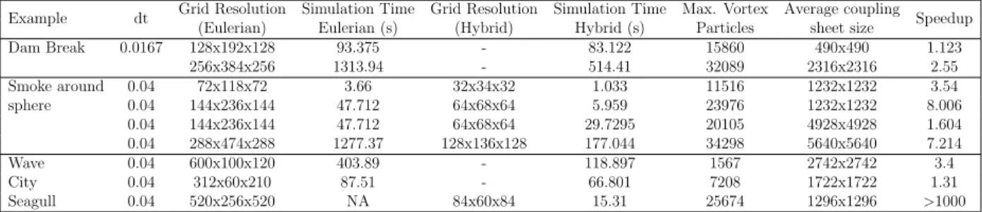
2.1 Single thread performance for my examples (All time values for one simulation step) . . . 32
LIST OF FIGURES
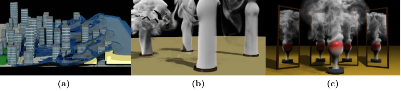
2.1 Examples of fluids simulated with my technique: (a) a city block hit by a
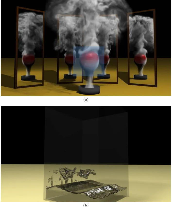
tsunami (vortex domain in yellow) (b) seagulls flying through smoke (c) smoke flow around a sphere. I achieve up to three orders of magnitude of performance
over standard grid-only techniques. . . 15
(a) . . . 15
(b) . . . 15
(c) . . . 15
2.2 Several seagulls flying through clouds of smoke to demonstrate airflow around their wings. On this scenes, my simulation achieved speedups of >1,000x . . 21
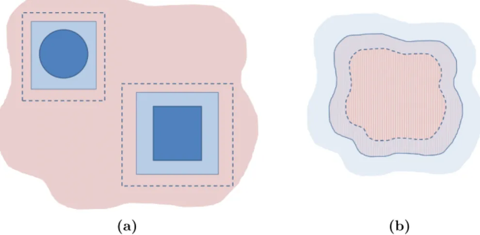
2.3 Decomposition of domain into vortex (red) and Eulerian grid (blue) subdo-mains for (a) single-phase flows, and (b) free-surface flows. Dotted lines denote grid region boundaries, while solid lines denote the vortex coupling sheet . . 25
(a) . . . 25
(b) . . . 25
2.4 Examples of fluid flow and domain decomposition (a) static, for single-phase flows, (b) dynamic, for free-surface flows changing with the topology of water extent . . . 37
(a) . . . 37
(b) . . . 37
2.5 The main steps of my method. . . 38
2.6 Dam Break example at t=0.48s using PIC(left) and FLIP(right) showing max-imum height reached by water . . . 38
(a) . . . 38
(b) . . . 38
3.1 Results without lookahead (left) and with lookahead (right) for 2 demo sce-narios. Crossing: (Top) shows two groups of agents seeking to exchange positions at simulation time t = 10s. Note how, with lookahead, the bigger group parts to allow smaller group through. Circle: (Bottom) shows agents on the edge of a circle heading to diametrically opposite points at simulation time t= 40s. Note significantly improved progress with lookahead. . . 40
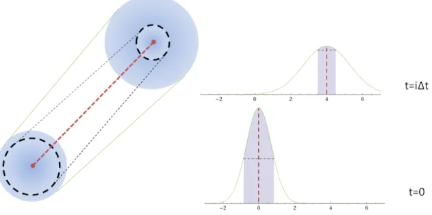
3.3 Effect of lookahead. Note how lookahead allows the orange agent to see the approaching crowd and adjust its velocity from preferred velocity vp to v by
incorporating information from the future crowd state at timet+ ∆t. . . 65
3.4 Lookahead Algorithm using LCA algorithm A. . . 66
3.5 Distant agents can be clustered for collision avoidance, cluster size being pro-portional to distance. Since possible collisions with distant agents lie in future timesteps, extrapolated future agent states have high uncertainty, and hence small effective radii, making individual avoidance inefficient. . . 66
3.6 Lookahead Algorithm using RVO. . . 67
3.7 My proposed inconsistency metricσis computed as the sum of the eigenvalues λ1, λ2 of the given deviation vectors δv (in red), which represents the variance of these deviations. The eigenvectors x1, x2 (in green) corresponding to these eigenvalues represent the principal components of the space of deviations. . . 68
3.8 4 way crossing of agents with 2000 agents. (a) Discrete (b) Discrete with lookahead (c) Continuum (d) Continuum with lookahead. Note lack of agent buildup in cases with lookahead. . . 69
(a) . . . 69
(b) . . . 69
(c) . . . 69
(d) . . . 69
3.9 Effect of Curtailing Lookahead in the circle (Top) and 4 groups (Bottom) demo. Solid lines show curtailed lookahead, while dotted lines show constant lookahead. Note how curtailing lookahead with a maximum metric value σmaxallows agents to reach their goals faster, as demonstrated by the reduced duration. In some cases, curtailing can double the improvement shown by lookahead (circle,imax = 16). Even with optimal choice ofmmax, I see benefits of 10%.. . . 70
3.10 4 groupsof agents in circular formation exchange their positions. Notice how lookahead (b) shows red and green agents moving around the built up region in the center and avoid getting stuck as is the case in (a). . . 71
(a) . . . 71
(b) . . . 71
3.12 Speed v.s. density plots for simulated crowds using (Top) traditional local collision avoidance, and (Bottom) long-range collision avoidance. Note how simulation with lookahead improves correspondence to speeds observed in the real-world data as compared to density, and how collision avoidance with lookahead demonstrates the same downward trend in speed with increasing density. . . 73
3.13 Crowd motion using (Top) real-world data, (Middle) Local collision avoidance, (Bottom) Long-range collision avoidance. . . 74
4.1 Continuum Simulation Algorithm for Crowd Turbulence . . . 82
4.2 Scene setup for Hajj simulations. The scene consists of two merging sets
of agents emerging from the inlets shown in the blue checkerboard pattern, following the path highlighted by dotted arrows and exiting via the wavy yellow outlet on the right. Corridor dimensions are shown by red arrows. . . 87
4.3 Representative trajectories taken by agents in the Hajj simulation to travel a distance of 8m in laminar (red, right), stop-and-go (black, middle) and turbulent flow (blue, left), with time rescaled to unity. . . 88
4.4 Temporal evolution of velocity components vx and vy. Under laminar flowvy
will remain close to zero. However, under turbulent flow, such as in this case, I observe motion that is orthogonal and even against the desired direction of motion (along the +x direction). . . 89
4.5 (a) Plot of average speed vs. density. Note that even though average speeds may be low at high densities, high variance implies that agent speeds may be significantly higher than the mean (b) Plot of crowd “pressure”P(x) = ρ(x) Varx(v) as defined by [Helbing et al., 2007]. I observe values greater than
0.02 at local densities of 7 people per m2 and higher, which are indicative of crowd turbulence. . . 90
(a) . . . 90
(b) . . . 90
4.6 Plot of crowd “pressure” overlaid with mean flow velocities for a time period of 3 seconds for (a) stop and go flow, and (b) turbulent flow. Note formation of irregular clusters as denoted by isocontour lines. Color bars show range of “pressures” observed; note that values greater than 0.02 do not arise in the occurrence of stop-and-go waves. . . 91
(a) . . . 91
4.7 Scene setup for Love Parade simulations. The scene consists of three merging sets of agents, emerging from the inlets shown in the blue checkerboard pat-tern. Agents from the bottom two inlets proceed towards the third inlet at the top and vice versa, following the paths highlighted by the dotted arrows. Corridor dimensions are shown by red arrows. . . 92
4.8 Plot of crowd “pressure” overlaid with mean flow velocities for a time period of 3 seconds for turbulent flow. Note formation of irregular clusters as denoted by isocontour lines. Color bars show range of “pressures” observed. . . 93
4.9 (a) Plot of average speed v.s. density. (b) Plot of crowd “pressure”. I observe values greater than 0.02 at local densities of 5.5 people per m2 and higher, which are indicative of crowd turbulence. . . 94
(a) . . . 94
(b) . . . 94
4.10 Plot of crowd “pressure” P(t) = hρ(t) Vart(v)ix in the Hajj scenario with
both discomfort and friction (top), and with discomfort alone (bottom). h·ix
denotes the mean computed over the entire scene. Note how discomfort alone is unable to recreate turbulent flow conditions. . . 95
4.11 Plot of the magnitude of the strain rate tensor k∇v + (∇v)Tk
F at t = 3s
Chapter 1: Introduction
From rolling crowds, rising smoke, to water in fountains and rivers, our world is full of
things that flow. These are very different from rigid objects like rocks, pieces of furniture etc. which maintain their shape. The key property of any flow is that it deforms continuously
with no consistent rigid shape. Under this definition, a number of other commonly observed
phenomena can be classified as flows. These include moving crowds of people, vehicular
traffic, and even granular media like sand and other grains. Owing to their omnipresence
nature, virtual environments often need to model flows for an immersive experience. This
dissertation focuses on efficient modeling and simulation of such flows.
Given their variable nature, a single model cannot describe all flows – but most flow
mod-els do have significant similarities, particularly in their underlying representations and
ap-proaches used to simulate them. A multitude of models already exist for simulating different
kinds of flows. For example, most Computer Generated Imagery (CGI) in movies uses fluid
simulation models based on the Navier-Stokes equations [Bridson and M¨uller-Fischer, 2007].
These models trace their lineage back to the middle ages, when siege warfare motivated
the study of flows to help understand the dynamics of moving large quantities of earth and
water. Thus began research into the problem of advection, which describes the transport of any media by bulk motion of the flow. The advection problem for a conserved property f by a velocity field u can be described by the following differential equation:
∂f
∂t +∇ ·(fu) = 0 (1.1)
This description covers everything from flowing water, to marching armies, and even to
how air affects projectiles like bullets and arrows traveling through it. For flows consisting
from one point in space to another. For these scenarios and others where the velocity is
incompressible, the advection equation can be simplified to the more well-known form:
∂f
∂t +u· ∇f = 0 (1.2)
For continuum flows like water solving the advection problem efficiently remains a key
con-cern.
Their continuously deforming nature makes continuum flow advection a significantly more
complex problem as compared to discrete rigid objects. Since the latter maintain shape and
form, their motion can be completely described by defining the velocity of any two points
on or within the object – or by two vectors at one point: velocity and angular velocity.
Velocity at any other point within the extent of the object can then be derived analytically.
This property does not hold for flows – velocity at any two points along a flow may not be
correlated. This difference allows flows to exhibit the variety of behaviors they exhibit, but
increases the complexity in simulating these very behaviors using a computer. Given initial
values for velocities, a flow model defines their time evolution – usually using differential
equations. A simulation then proceeds by updating the simulation state – velocity, position
etc. – over short intervals of time, called time steps.
However, advection forms only one part of flow models. The flows discussed in this
thesis also share one other component, one that maintains density. In fluids this is the
“incompressibility” constraint, which mandates that a fluid must maintain a constant density.
This constraint is traditionally modeled using apressure force applied on the velocity field ˜v resulting from advecting the velocity by itself. The nature of this pressure force is repulsive
in high-density regions, and attractive in low-density regions. Mathematically it takes the
form of a corrective term:
vt+∆t = ˜v−∆t1
ρ∇p (1.3)
gradient of pressure, which is computed as the solution to the equation:
∆t ρ ∇
2p=−∇ ·v˜ (1.4)
This equation enforces the incompressibility constraint, and belongs to the class of elliptic differential equations. The key characteristic of such equations is that their solution at any
point in space depends on the solution at every other point in space. This implies that
information in an elliptic differential equation travels at infinite speed throughout the entire
domain. An intuitive analogue to this is to consider a force applied on a rigid object, where
the entire object moves while maintaining its rigid structure without deforming. The lack of
deformation is due to the near-instantaneous propagation of the effects of the force through
the object. Collision avoidance in crowds is also similar in nature; it ensures that virtual
pedestrians do not collide with one another by maintaining a minimum distance, and thus
local crowd density does not increase above a maximum threshold value.
As we increase the scale of the problem – be it in terms of spatial scale or increased
detail – the complexity of the simulation increases, which translates into inaccurate results,
significantly slower simulation, or both. There may be multiples sources of this
complex-ity. The first source is the validity of the model itself. Motion of certain flows can exhibit
patterns that cannot yet be captured using differential equations. Crowds of pedestrians for
instance, can change their velocities discontinuously based on individual decisions of those
very pedestrians. However, models do exist for simulating the navigation of virtual
pedestri-ans in a medium-sized domain – like a small hall for instance – with an average pedestrian
density of up to 3−4 people perm2. However, the same models are unable to recreate crowd
behavior when domains are significantly larger (e.g. a large battlefield), or when crowd
den-sity is higher (e.g. in congested conditions when stampedes may occur). Existing crowd
navigation models cannot model such scenarios since the criteria for pedestrian navigation
Thus, for flows such as crowds, any proposed model should be able to closely match observed
real-world data.
The second aspect of this problem is the impact on performance. In order to make
large-scale flow simulation viable, performance of proposed models must large-scale with increasing
detail or size. In that context, the problem of solving elliptic differential equations like
Eqn.(1.4) can be computationally more complex than advection. Advection relies purely on
local information, like local velocity and local value of the property being advected. On the
other hand, elliptic problems like incompressibility require incorporating information from
the entire region in which the flow exists, i.e. the domain of the simulation. This global dependence is commonly modeled as a system of equations (like for equation (1.4)), or a
global optimization problem as in the case of collision avoidance in crowds. In order to
understand issues in scaling performance, it is important to understand the discretizations
used by most models.
1.1 Modeling Flows
Any flow model must begin by defining certain properties: the domain, or the extent of
the flow, and the velocityvand density ρwithin the domain. For the flows discussed in this dissertation, the most common approach is to define sample points where these properties
are explicitly defined, then use a set of basis functions to interpolate them at any other
point in space. There are multiple options for choosing sample points, a common example
being uniformly spaced samples along an orthogonal basis. The resulting discretizations
are known as finite difference methods. These are popular since they are easy to analyze mathematically for correctness, and amenable to parallelization due to the regular nature
of sample positions. Apart from how sample points are chosen for a discretization, one
other important distinction is whether these sample points are static over time, or can move
that move with the flow. In the latter case, particles also serve as markers on where the flow
exists, removing the need for defining the property explicitly.
This dissertation looks into the problem of simulating flows at large scales using verifiably
correct models that are efficient and scalable on desktop computers. However, to understand
the complexity this poses, we must first understand these two representation classes and their
impact on computational complexity.
1.1.1 Eulerian Representation
Eulerian representations discretize the flowdomain, i.e. the space in which the flow exists, and may exist in the future. To do so, they define stationary points in the domain, where flow
properties are sampled; values at other points in space are defined by interpolating sample
values. Defining the behavior of a flow over time then requires describing the variation of
flow properties at sample points over time. To illustrate this principle, consider a simple
example of a stream with water flowing over rocks. Assuming the stream flow is in a stable
state, the velocity of water at any particular point in the stream does not change with
time. As a result, using an Eulerian discretization for this case, velocity values at any
sample point will remain constant over time, even though water is moving. In addition, a
simulation may focus on a small part of the stream – its domain – simulated with appropriate
velocity boundary conditions. Simulation may then be performed by choosing sample points
distributed uniformly throughout the domain.
The choice of the simulation domain and the granularity of discretization defines an
Eulerian discretization. The chosen domain must be large enough to encompass a region
where flow features of interest occur. However, due to limited computational resources, the
placement and number of sample points is also a key decision. For most flow models, the
domain of simulation can be made larger while keeping the number of sample points constant,
in accordance with stability and accuracy constraints. Though not required explicitly, most
Eulerian models fix the domain, sampling positions, and desired time step at the beginning
of the simulation for efficiency reasons. The static nature of these setups presents a problem
for large scale flows, as covering the entire region where interesting flow features may occur,
with sufficient resolution and a sufficiently small time step requires a prohibitive number of
sample points.
The smallest scale resolved by Eulerian discretizations is defined by the minimal
spac-ing between sample points. Thus, given certain computational restrictions, most Eulerian
discretizations balance domain size with the separation between sample points. Thus,
flows can either be sampled at fine granularity in small domains, or coarsely in larger
domains [Fedkiw et al., 2001]. Adaptive discretizations are possible and have been
pro-posed where sample points are added and removed based on the expected local details
[Losasso et al., 2004,Adams et al., 2007]. Though computationally efficient as compared to
na¨ıve discretizations with uniformly spaced sample points, these methods have additional
costs as well. Mathematical analysis of the method becomes more complex, and the
irregu-lar structure makes parallelization more challenging. In addition, choosing the appropriate
sampling rate is a non-trivial undertaking, since predicting when and where detailed flow
phenomena may appear is hard. This leads to constraints on the spatial variation of
sam-pling rates. For example, in structures like octrees, samsam-pling rates can vary only by a factor
of two for adjacent samples for quality reasons, as heuristics maintaining sampling rates do
not permit a larger variation.
This restriction on sampling rate variation has implications when simulating large scales.
At sufficiently large scales, uniform sampling like the one chosen for the simulated stream
or even adaptive sampling becomes untenable, as the spatial resolution of the flow becomes
too low to resolve any features of interest, and choosing sufficient sample points becomes
computationally intractable. For example, the chosen sampling rate may be insufficient
pedestrian in a dense crowd.
1.1.2 Lagrangian Representation
An alternative approach to sampling flows is to follow a methodology similar to that
used for rigid bodies. In such Lagrangian discretizations, sample points are advected with the flow itself. This leads to a very different definition of the domain, which now defines
sample points not in the space which the flow may occupy, but only in the space the flow does occupy. For flows like water and crowds where spatial extent is restricted, Lagrangian discretizations can reduce the memory footprint of sampling. However, temporal progression
of flow properties changes in such a discretization. To illustrate this, consider the previous
example of the stream again. If the sample points where velocity is measured are Lagrangian
and move with the stream flow, then velocity samples will show a temporal variation. At
different time instants, the same Lagrangian sample may measure the velocity of water deep
inside the stream, over a rock feature, or even falling off a cliff. To reconcile this viewpoint
with the previously discussed Eulerian view, derivatives with respect to time are defined
differently in the Lagrangian viewpoint, usingmaterial derivatives. These can be related to Eulerian derivatives by the following equation:
Dx Dt =
dx
dt +v· ∇x (1.5)
The above equation expresses the rate of change of a property as observed from a frame of
reference moving at velocity v as the rate of change of the property w.r.t. a static frame of reference plus the effect of the motion – the spatial gradient of the property in the direction of
motion. One complication that arises from the use of Lagrangian discretizations is ensuring
consistent spacing of sample points. Over time, sample points can get clustered, leading
to instability and accuracy issues. To remedy this, sample points must be redistanced or
nearby sample points can be bounded.
In cases where the flow domain is a superset of the flow extent, Lagrangian discretizations
may have a lower memory footprint than Eulerian methods. For example, a mass of water
moving through a pipe always occupies a small finite region within the pipe. Over a period
of time, though the flow may occupy a large segment of the pipe (the flow domain), at any
instant of time the flow extent is always much smaller. Lagrangian discretizations for such a
flow can discretize the smaller flow extent, while a static Eulerian discretization must work
with the flow domain. In spite of these savings however, the growth rate of this memory
footprint with increasing scale or detail remains high for both classes – growing at least
linearly with the area (in 2D) or volume (in 3D) of the flow, and at quadratic or cubic rates
with detail respectively.
Increasing memory footprint of the discretization used to resolve finer detail or increased
spatial scale poses a computational issue for flow simulations, particularly due to the elliptic
problems discussed earlier, which need to access a significant percentage of this memory
foot-print multiple times. Thus, to maintain reasonable throughput in the simulation, memory
bandwidth must be sufficiently large.
1.2 Utilizing Parallel Desktop Architectures
To understand why larger memory footprints are poorly suited for shared memory
archi-tectures like desktops, it is necessary to look at the problem from an architecture perspective.
Recent developments in processor architectures have attempted to increase computational
performance by adding additional cores to processors, allowing more tasks to be run in
parallel. This trend is evident in all compute architectures, including CPUs, as well as
co-processors like the GPUs and the Intel® Xeon Phi. This push is motivated by the fact that a lot of workloads relevant for real-world applications are compute-bound, i.e. their performance is limited by the number of computing cores. However, with these parallel
bandwidth bound, where computing cores spend most of the time waiting for data to be
de-livered by the memory subsystem, thus adding more cores does not help speed up the overall
execution time of the simulation. This situation happens most often in elliptic problems
noted previously, where systems of equations may need to access and update large regions
of memory repeatedly in a global step.
Though this can be addressed by improving memory subsystem throughput, it is a
com-plex problem, bounded by the cost of adding high-speed memory units close to computing
cores. The solution commonly used is a hierarchy of caches, with slow DRAM chips at
the bottom. In this hierarchy, latency and throughput limitations of DRAM are hidden by
multiple levels of caches, each higher level of cache having lower latency of access, higher
throughput, but smaller size. Owing to the cost constraint of adding bigger caches, in order
to efficiently utilize these increasing computational resources, algorithms for flow simulation
need to be architecture-aware in two key aspects.
First, any proposed algorithms need to be amenable to parallelization, preferably with
minimal interaction or dependencies between parallel threads. The latter desire stems from
the fact that highly parallel architectures like GPUs work optimally when each thread can
run independently. Secondly, the working set of the algorithm and its overall memory
band-width requirements need to be small. Ensuring this constraint helps ensure that at larger
scales, computation does not become memory-bound, and the simulation can fully exploit all
available compute cores. A smaller working set has a higher likelihood of remaining resident
in high-speed caches, reducing latency of access, and improving overall throughput.
To incorporate these performance aspects, this dissertation proposes novel algorithms for
scenarios where na¨ıvely scaling existing models is untenable – either since the model cannot
accurately capture phenomena at these scales like in the case of crowds, or since it leads
to memory-bound computation as in the case of fluids. In case of fluids, this dissertation
addresses computational scaling at large spatial scales. For crowds, it looks at modeling
1.3 Coupled Hybrid Simulation
In this dissertation I propose the use of coupled Eulerian-Lagrangian models for efficiently
simulating phenomena at multiple spatial and temporal scales. These models are capable of
simulating previously infeasible flow scenarios, as well as replicating certain flow behaviors
not captured by existing models. An additional feature of these models is a lower memory
footprint at large scales resulting in improved performance on parallel architectures, allowing
the simulation of flows at larger scales than existing models under a limited computational
budget.
These hybrid models can be used to simulate a number of real-world scenarios of interest
in computer graphics and other fields, notably:
Simulating fluids at large scales: Existing Eulerian models for simulating flu-ids scale poorly, with memory requirements growing with the 3rd power of scale, and
computational requirements growing with the 4th power. These make large-scale
sim-ulations highly inefficient, to the extent that more computational power does little to
increase performance.
Flow of pedestrians in large environments: Most crowd models use a Lagrangian discretization, where each pedestrian is considered a discrete entity. These models
include a trade-off between performance and accuracy w.r.t. distance – performing
collision avoidance up to a nearby threshold distance. This is suitable for most
real-world scenarios, but provides inaccurate results when the scene domain is large, while
considering a larger threshold distance makes the algorithms scale quadratically with
number of pedestrians. As a result, simulations are unable to maintain the desired
real-time simulation rate.
assume that pedestrians can avoid contact with others. However, in extremely
con-gested environments where crowd density is very high (5−6 people perm2 and higher),
pedestrians collide almost continuously with others, giving rise to chaotic emergent
be-havior like stampedes, which cannot be replicated by existing models.
This dissertation discusses these scenarios in detail and proposes coupled
Eulerian-Lagrangian models for efficient simulation.
1.4 Thesis Statement
My thesis statement is as follows:
Complex large-scale flows such as crowds and fluids can be simulated efficiently and scal-ably on current desktop hardware using novel algorithms that simulate multiple spatial and temporal scales using coupled Eulerian and Lagrangian discretizations.
To support this thesis, I present three methods; one method to efficiently simulate fluids
at scale scales, and two methods to accurately simulate crowds at larger spatial scales, and
at high densities.
1.5 Main Results
Large-scale Fluid Simulation
Simulating fluids in large scale scenes with high visual fidelity using state-of-the-art
meth-ods can lead to high memory and compute requirements. Since memory requirements are
proportional to the product of domain dimensions, simulation performance is limited by
memory access, as solvers for elliptic problems are not compute-bound on modern desktop
systems. This is a significant concern for large-scale scenes. To reduce the memory footprint
and memory/compute ratio, a different representation, called vorticity can be used, where vorticity represents rotational motion in fluid flow. When represented using a Lagrangian
In Chapter 2, I propose a hybrid model exploiting this insight; Using Lagrangian vortex
singularity elements in the fluid interior, coupled with an Eulerian velocity-based simulation
near all interfaces (with air or solid objects). The key benefit in using this model is that
the memory footprint of the simulation is reduced significantly, as instead of discretizing the
fluid volume, we discretize its surface, with additional cost proportional to the amount of
vortex features.
The main contributions of my work are:
Demonstration of a hybrid simulation algorithm that utilizes coupled Eulerian and
Lagrangian discretizations at different spatial scales to simulate fluids
A novel coupling algorithm that conserves vortex features in the fluid as well as mass
and momentum of the flow
An algorithm that can simulate large gaseous flows many orders of magnitude faster
than existing methods, with significant gains for liquid flows
These results were published in [Golas et al., 2012].
Long-range collision avoidance in crowds
Local collision avoidance algorithms in crowd simulation often ignore virtual pedestrians
(agents) beyond a neighborhood of a certain size. This cutoff can result in sharp changes
in trajectory when large groups of agents enter or exit these neighborhoods. In this work, I
exploit the insight that exact collision avoidance is not necessary between agents at such large
distances, and propose modeling the avoidance problem at multiple spatial and temporal
scales to perform approximate, long-range collision avoidance. This model can be used
with both Eulerian and Lagrangian discretizations, as well as coupled Eulerian-Lagrangian
discretizations for maximum efficiency.
A model that performs collision avoidance approximately at multiple spatial and
tem-poral scales for both Eulerian and Lagrangian discretizations
A hybrid model that utilizes both Eulerian and Lagrangian discretizations with coupled
avoidance models to simulate collision avoidance in crowds at a wide range of crowd
densities
Simulated behavior generated by this hybrid model shows close correspondence to
observed real-world crowd behavior
Demonstration that efficient implementations of these models can simulate thousands
of virtual pedestrians at interactive rates on current CPUs
This work was published as [Golas et al., 2013b, Golas et al., 2013a]
Crowd Turbulence in High-density crowds
With the growth in world population, the density of crowds in public places has been
increasing steadily, leading to a higher incidence of crowd disasters at high densities. Recent
research suggests that emergent chaotic behavior at high densities – known collectively as
crowd turbulence – is responsible. Thus, a deeper understanding of crowd turbulence is
needed to facilitate efforts to prevent and plan for chaotic conditions in high-density crowds.
However, it has been noted that existing algorithms modeling collision avoidance cannot
faithfully simulate crowd turbulence.
I propose a hybrid model for simulating crowd turbulence, that couples a Lagrangian
agent model with an coarse Eulerian model for frictional forces arising from pedestrian
interactions. The main results of this work are:
A novel model that couples a fast-varying Lagrangian agent model with a slow varying
Simulated behavior generated by this model shows close correspondence to observed
real-world crowd behavior and known metrics
Scalar implementation capable of interactive performance on current desktop CPUs
This work was published as [Golas et al., 2014].
1.6 Organization
The remainder of this dissertation is organized as follows. The discussion of hybrid models
begins with the simulation of fluids at large scales in Chapter2. This is followed by my work
on collision avoidance behavior of crowds at large scales in Chapter 3. Finally, I discuss a
model for simulating chaotic behavior in crowds at high-densities in Chapter 4. Chapter 5
concludes this dissertation by presenting a summary of this work, its contributions, and a
Chapter 2: Large-scale Fluid Simulation using Velocity-Vorticiy Domain Decomposition
2.1 Introduction
State-of-the-art methods for fluid simulation, including velocity-based Eulerian methods
and smoothed particle hydrodynamics, model the entire spatial extent of the fluid. Dis-cretization of this space is often chosen to be able to sample sufficiently fine details under
the restriction of limited computational resources. As a result, scenes with large spatial
scales can only be simulated to coarse detail on PCs, relying on procedural methods to infuse
detail. The simple computational kernels of these methods are largely memory-bandwidth bound, since domains of interest cannot reside in caches of current generation CPUs, and computational complexity cannot mask the cost of memory accesses. An alternate approach
to modeling fluids is to model fluid detail, represented by the vorticity of the fluid, i.e. the curl of the velocity field. For incompressible flows, vorticity can be compactly represented
by Lagrangian singularity elements. They are thus free of numerical dissipation, which can
be a significant issue with Eulerian methods, and do not need to explicitly model the
pres-(a) (b) (c)
sure of the fluid. Though this leads to computational savings for scenes with unbounded
fluid, robust and efficient modeling of obstacles or free-surfaces with two-way coupling using
vorticity methods is challenging. Vortex singularity elements also serve as intuitive models
for visual fluid detail, e.g. a smoke ring can be modeled as a vortex curve or filament.
These aspects make detail modeling of fluids with vortex singularity elements attractive, especially for large-scale scenes. To extend the applicability of these methods to free-surface
fluids and scenes with deformable elements, I propose a hybrid domain-decomposition
ap-proach. Since Eulerian methods are adept at modeling such surfaces, coupling them with
vortex methods can provide a robust, flexible, and efficient approach to fluid simulation.
Particularly for scenes with large spatial scales but concentrated regions of detail, my
ap-proach can provide substantial computational and memory savings with reduced numerical
dissipation, allowing simulations with more detail than previously possible.
It also poses significant challenges, the biggest of which is coupling heterogeneous methods
in the same simulation while ensuring a consistent velocity field that matches the actual
fluid velocity. I address this problem by separately coupling fluid flux and vorticity across
simulation boundaries. I propose an iterative coupling algorithm that matches fluid flux
across boundaries using appropriate boundary conditions for grid simulations and by creating
vortex singularities on the boundary for vortex simulations. To accurately transfer vorticity
across boundaries, I use a novel vortex particle creation algorithm and velocity boundary
conditions for advection. It is important to note that maintaining vortex surface elements
is computationally expensive and numerically ill-conditioned if surface mesh quality is poor.
I develop an approach that addresses both of these issues by constructing meshes using
grid faces, and efficiently computing fluxes induced by these face elements, even allowing
pre-computation. I extend hierarchical approach of [Lindsay and Krasny, 2001] for faster
computation of flux induced by vortex particles and surface elements.
Main Results: The key contributions of this work are:
com-pact vortex basis with Lagrangian elements in the interior of the fluid, while enforcing
arbitrary boundary conditions such as nonrigid obstacles and free surfaces using an
Eulerian grid representation near boundaries;
a novel two-way coupling between Eulerian Navier-Stokes simulations and Lagrangian
vorticity simulations, which conserves vorticity over time and ensures continuity in the
velocity and vorticity fields;
a sampling algorithm to create a vortex particle representation of a given velocity field
by minimizing residual in the L2 norm; and
an efficient and well-conditioned approach to computing strength of vortex surface
elements, and an O(mlogm) algorithm to evaluate flux using hierarchical methods.
The coupling techniques introduced in this chapter are quite general and can be used
to connect different kinds of fluid simulation techniques in a heterogeneous domain
decom-position framework. When applied to grid-based and vorticity-based methods, this method
enables efficient simulation of large fluid volumes using a vorticity representation while
sup-porting rich and complex interaction at boundaries. I demonstrate the benefits of this
approach on several large-scale scenes (see Fig. 2.1) which would have a prohibitive
compu-tational cost using existing techniques.
These results were published in [Golas et al., 2012].
2.2 Related Work
Physically-based simulation of fluids has been a major focus of computer graphics research
over the past decade. In this section, I briefly review the work in this area that is most
further classified in orthogonal categories based on the type of discretization, i.e. Eulerian
or Lagrangian methods.
2.2.1 Velocity-based methods
Most of the de facto standard techniques for fluid simulation in computer graphics use a velocity-based representation. In such methods, one solves a discretization of the
Navier-Stokes equations, which describe the evolution of the velocity field of a fluid over time.
A popular approach to solving these equations is by using finite difference methods
on Eulerian grids — this was introduced to computer graphics by the pioneering work
of Foster and Metaxas [Foster and Metaxas, 1996]. Stam [Stam, 1999] proposed
semi-Lagrangian advection schemes to allow for unconditionally stable fluids, and Foster and
Fedkiw [Foster and Fedkiw, 2001] developed methods for producing realistic, robust
liq-uid surfaces in simulations. These methods have the advantage of being simple to
im-plement and producing visually compelling results, including interactions with rigid and
de-formable objects [Chentanez et al., 2006, Batty et al., 2007, Robinson-Mosher et al., 2008].
Similar techniques have also been proposed using tetrahedral meshes [Wendt et al., 2007,
Klingner et al., 2006, Chentanez et al., 2007] instead of rectilinear grids. However,
Eule-rian simulators have traditionally faced two challenges. First, they suffer from
signifi-cant numerical dissipation, typically exceeding the desired viscosity in the fluid, causing
flow detail to be undesirably damped out. Recent developments in improved advection
schemes offer benefits in this aspect [Kim et al., 2007,Selle et al., 2008,Mullen et al., 2009,
Lentine et al., 2011, Zhu and Bridson, 2005], while techniques for introducing additional
detail have also been proposed [Fedkiw et al., 2001, Selle et al., 2005, Kim et al., 2008,
Narain et al., 2008, Schechter and Bridson, 2008, Pfaff et al., 2010]. However, a second,
more fundamental challenge is that Eulerian methods require voxelization of the entire
sim-ulation domain. The elliptical pressure projection operator needed to solve these
large computational and memory requirements for expansive scenes. Some recent work has
attempted to address this issue, with level-of-detail representations [Losasso et al., 2004],
coarse grid projections [Lentine et al., 2010], and model reduction [Treuille et al., 2006b,
Wicke et al., 2009], but these are often incompatible with techniques for reducing dissipation.
An alternative approach is that of smoothed particle hydrodynamics, which models the
fluid volume as a system of particles with pairwise forces between them. This approach has
been employed for interactive simulation of liquids [M¨uller et al., 2003]. Similar to
Eule-rian grids, these methods can lead to a large number of particle primitives to sample fluid
extent. In addition, enforcing incompressibility correctly can be expensive, owing to
ir-regular computational elements. These concerns have been addressed partly with adaptive
sampling [Adams et al., 2007] and predictive-corrective schemes for incompressiblility
pro-jection [Solenthaler and Pajarola, 2009]. Sin et al. [Sin et al., 2009] proposed a point-based
approach that combines features from particle-based and grid-based methods. However, for
the large scales under consideration, computational costs remain substantial for all such
techniques.
2.2.2 Vorticity-based methods
Vortex simulations are a class of methods which were originally devised for aircraft wing
design, and have recently begun to receive attention in computer graphics as well. These
methods model the evolution of fluid vorticity, which is the curl of the velocity field, in-stead of velocity itself. With the exception of Elcott et al. [Elcott et al., 2007]’s Eulerian
approach representing vorticity on a tetrahedral mesh, most of the methods in this category
are Lagrangian, using singularities with the Green’s function of the Laplace operator.
In this formulation, singularity methods can be applied, representing the
vorticity distribution as a superposition of singularities such as particles
[Chorin, 1973, Park and Kim, 2005], curves/filaments [Angelidis and Neyret, 2005,
excellent basis functions for fluid velocity for a number of reasons. They offer a compact
and exact representation of fluid velocity in unbounded domains, automatically ensure
incompressibility, and are immune to numerical dissipation. Due to their Lagrangian nature,
vortex singularity methods also allow easier user control of the simulation as compared to
grid methods. These features have made these methods popular for interactive simulations
[Angelidis et al., 2006, Weißmann and Pinkall, 2010]. Curve or filament representations
also ensure incompressibility of vorticity, but can only model inviscid fluids. This is not the
case with vortex particles, which allow viscous fluids to be modeled, at the cost of a slightly
compressible vorticity field. The divergence-free constraint can be enforced iteratively
through particle strength exchange methods [Cottet and Koumoutsakos, 1998], which can
also model viscosity.
Enforcing boundary conditions requires the solution of a dense linear system. Though
capable of arbitrary accuracy — conditions are enforced at mesh resolution — for nonrigid
obstacles, precomputation of the linear system is impossible, which makes these the
limit-ing factor in vortex simulations. Also, due to the slimit-ingular nature of vortex slimit-ingularities,
proximity of elements has a major impact on the conditioning of this linear system, to the
extent of rendering the system unsolvable due to poor conditioning. Large variations in the
size of elements have a similar effect on conditioning. These issues make efficient and robust
modeling of nonrigid obstacles non-trivial. It is also difficult to model the dynamics of free
surfaces in this framework.
While there have been a number of hybrid simulation techniques combining, for example,
rectilinear grids with tetrahedral meshes [Feldman et al., 2005], or grids with particle-based
methods [Losasso et al., 2008], all these work solely with velocities, and I am aware of no
work in computer graphics that allows combining velocity- and vorticity-based methods in
the same simulation.
The remainder of the chapter is organized as follows. The hybrid domain decomposition
Figure 2.2: Several seagulls flying through clouds of smoke to demonstrate airflow around their wings. On this scenes, my simulation achieved speedups of >1,000x
vortex simulations in Section 2.4. Finally, results and analysis of my implementation are
described in Section 2.5.
2.3 Hybrid Fluid Simulation
Given velocity-based and vorticity-based methods have complementary advantages, I
pro-pose a hybrid approach that combines the respective strengths of both techniques. In
partic-ular, many different techniques have been proposed to support different types of boundary
conditions for velocity-based methods, including free surfaces, deformable and thin objects,
and two-way coupling. On the other hand, vorticity-based methods can compactly
repre-sent effectively infinite volumes of fluid where detail in the fluid motion is spatially limited.
Therefore, I propose to combine both methods through a domain decomposition approach
(Section 2.3.2), representing the fluid using velocity-based methods near boundaries such
region of the fluid.
However, the disparate nature of velocity and vorticity methods makes it challenging to
combine them into a single heterogeneous simulation. An essential problem is that of
cou-pling together the two representations at the interface between them, so that they represent
a consistent velocity field for the entire fluid. I present a novel two-step coupling algorithm
to address this problem: first matching normal velocities at the interface using an
alternat-ing scheme (Section 2.3.3), and then transferring vorticity information across subdomains
through particle seeding (Section 2.3.4). As I show below, matching both velocity and
vor-ticity across the interface is necessary to obtain a consistent and convergent simulation in
this framework.
2.3.1 Subdomains
My simulation consists of Eulerian (Gi) and Vortex (Vi) subdomains. For notational
simplicity, I use G and V to refer to the union of all Eulerian subdomains and Vortex sub-domains respectively. Eulerian subsub-domains model the Navier Stokes equations using uniform
grids, with velocity u sampled on a staggered grid. Operator splitting is used to integrate each term one by one, with a BFECC Semi-Lagrangian scheme for advection, explicit
inte-gration for external forces, and a sparse Poisson solve for enforcing incompressibility using
pressure. Advection and Incompressibility solve steps take volume flux boundary conditions
from the hybrid simulator, instead of zero flux enforced in traditional solvers. For more
details I refer the reader to [Bridson and M¨uller-Fischer, 2007, Carlson, 2004].
Vortex subdomains (Vi) model the evolution of vorticity ω=∇ ×u, using the vorticity form of the Navier Stokes equations:
∂ω
∂t + (u· ∇)ω = (ω· ∇)u+ν∇
2ω, (2.1)
under the assumption of no density gradients. Under this formulation, velocity can be
expressed using the Green’s function of the Laplace operator, giving rise to the Biot-Savart
formula:
u(x) = 1 4π
Z
R3
ω(z)× x−z
kx−zk3dz. (2.3)
for a vorticity distribution in an infinite domain. Note the absence of a pressure term, as the
velocity so defined is incompressible by definition. As mentioned before, this distribution
can be represented as a superposition of discrete primitives such as points (particles), curves
(filaments), or surfaces/meshes (sheets) giving rise three types of vortex singularity methods.
I use a particle representation owing to its ease of use, and the possibility of modeling
viscosity, which is not possible using filaments. Also, due to poor long term stability of ideal
singularities, regularized singularities or “vortex blobs” are typically preferred. A popular
choice is the Rosenhead-Moore kernel, a regularized form of the Biot-Savart kernel with a
constant smoothing radius a to give
u(x) = 1 4π
Z
R3
ω(z)× x−z
(kx−zk2+a2)3/2dz. (2.4)
The smoothing radius governs the concentration of vorticity represented by a vortex blob,
which affects the scale of vorticity features that can be represented by it.
The vortex particle algorithm proceeds by advecting vortex particles, perturbing
par-ticle strengths to model vortex stretching and viscosity, and creating vortex sheets
to model obstacles. Particles whose strength falls below a minimum threshold are
culled. For more details about advection, stretching and viscosity, I refer the reader to
[Cottet and Koumoutsakos, 1998]. Obstacles are modeled by creating vortex sheets on their
surface. [Weißmann and Pinkall, 2010] propose creating filaments along the edges of a
polyg-onal mesh for this purpose, where the strength (Γi) of each filament (fi) is determined to
enforce zero flux through each face of the mesh, i.e. P
In the hybrid case, I create sheets to match a non-zero flux, resulting in the equation for
the strength of each filament: P
iΓif luxi(fj) +f luxV(fj) =f luxG(fj). In case of multiple vortex domains, either all vortex sheets can be computed using one solve, or by iteratively
solving for the strength of each vortex sheet separately. This choice usually depends on
whether linear systems for each component can be precomputed or not.
2.3.2 Hybrid Domain Decomposition
In my hybrid approach, I divide the simulation domain into a number of non-degenerate,
overlapping subdomains, each of which is simulated using either the vortex method or
Eule-rian Navier-Stokes simulation.
It is natural to define one large region V, consisting of the interior of the fluid at least a distance d away from boundaries, on which the vortex method is applied. This region
consists of one or more disjoint subdomains Vi. The other subdomains, labeled Gi, use Eulerian Navier-Stokes simulations, and may contain boundaries such as static or moving
obstacles and free surfaces. I assume that all Eulerian subdomainsGi are disjoint from each other (if not, I may merge any grids that overlap), and each of them overlaps with the vortex
subdomain V, in order to apply my coupling algorithm. Thus, the burden of supporting various boundary conditions is lifted from the vortex method, and placed on grid-based
methods for which numerous techniques are available.
This decomposition is illustrated in Figure 2.3. For single-phase simulations like smoke,
the domain consists of grids immersed in a vortex simulation, with the vortex domain
ex-tending to a user-specified distance d inside every grid. For free-surface simulations like
water, the vortex simulation is embedded inside an Eulerian grid, with the boundary of the
vortex domain being a distance d inside the fluid surface. As boundaries move, so do their
corresponding subdomains, so that at all times the boundaries are contained entirely within
grids and remain at least a distance d from the extent of the vortex subdomain.
(a) (b)
Figure 2.3: Decomposition of domain into vortex (red) and Eulerian grid (blue) subdo-mains for (a) single-phase flows, and (b) free-surface flows. Dotted lines denote grid region boundaries, while solid lines denote the vortex coupling sheet
boundary conditions. That is, the boundary of the vortex subdomain, which is a surface
that lies entirely within the grid, is treated as an obstacle whose normal velocities are given
by the grid velocity field, and a vortex sheet is computed on this surface to match the
corresponding fluxes. Thus, the velocity field can be evaluated at any point in the interior
using the Rosenhead-Moore kernel (2.4).
I define the timestepping scheme of the hybrid simulation as follows. Each subdomain is
advanced independently over one time step ∆t while assuming that velocities in the others
are constant. Assuming constant velocities in other subdomains introduces an error on the
order of O(∆t) in both vortex and grid regions: in the vortex region because boundary
conditions are determined by the grid; and in the grid because advection carries velocities
in from the vortex region. In general, this magnitude of error is acceptable because the rest
of the simulation (like most techniques for fluid simulation in graphics) is also first-order
accurate. At the end of the time step, I couple the simulations back together by matching
normal velocities at the boundaries, thus enforcing incompressibility, and matching vorticity
in the interior of the overlap region. It can be shown that when the overlap region is simply
vorticity in the interior, they must be identical [Cantarella et al., 2002]. For overlap regions
with complex topologies, additional circulation constraints are needed. Thus, I can ensure
that the combined simulation is consistent: where the grid and the vortex domains overlap,
they agree on the fluid velocity.
In the following two subsections, I describe my proposed coupling techniques in more
detail.
2.3.3 Velocity coupling
Each Eulerian solver stores a velocity field which determines the velocityuGi at any point within its grid Gi. Similarly, the vortex method determines the velocity uV at any point
in its subdomain V. By allowing domains Gi and V to overlap, I can enforce consistency between the corresponding simulations by ensuring thatuGi anduV are equal in the overlap region Oi =Gi∩V.
To enforce this constraint, I recall that the velocity field in any region is uniquely
deter-mined by the distribution of vorticity within it, and the flux at the boundaries of the region.
Therefore, discrepancies between the velocities seen by different subdomains can only occur
from having incorrect vorticity information in the interior or incorrect flux at the boundary.
Assuming consistent vorticity in the overlap region, I need to ensure that flux across the
boundary of the overlap region is consistent, i.e. velocity induced by both simulations is the
same uGi =uV at the boundary .
Velocity can be matched at∂Gi by enforcing the desired velocity as boundary conditions
for the incompressibility projection step. To do the same with vortex simulation requires
the creation of a vortex sheet S to match normal flux through ∂V, i.e.
(uS+uV)·n=uGi·n (2.5)
Thus the velocity coupling can be formulated as a fixed point iteration, one iteration of
which can be expressed as follows:
1. Determine the velocity uV+uS at the boundary ∂Gi of the Eulerian subdomain
2. Using uV+uS as the boundary condition, perform the incompressibility projection on
the grid Gi
3. Determine the velocity uGi at the boundary ∂V of the subdomainV 4. Compute strength of the vortex sheet S to match vortex velocityuV to uGi
Coupling iterations are performed till uG and uV + uS converge. For coupling multiple
Eulerian subdomains with the vortex subdomain, this iteration can be performed in lockstep
for every pair of overlapping subdomains.
This algorithm belongs to the class of methods known as the Schwarz alternating methods
[Toselli and Widlund, 2004], which are commonly used in domain decomposition methods.
Schwarz alternating methods are guaranteed to converge to a unique solution for second order
PDEs, and thus this iteration ensures that the velocity field is consistent at the boundaries
of all subdomains, and consequently in the entire domain.
2.3.4 Vorticity exchange
Velocity coupling on the subdomain boundaries will yield consistent velocities over the
entire overlap region only if the vorticities seen by both representations are equal. However,
even if the vorticities are equal in the initial conditions, they will gradually go out of sync
over time, as vorticity is transported into the overlap region through advection. Therefore,
to ensure consistency at all times, I need to account for this by exchanging vorticity between
the grid and the particle domains. I derive this procedure by considering the two cases
where vorticity is brought into the overlap region from the vortex particles and from the grid
From the vortex particle domain, vorticity enters the overlap region when a vortex particle
flows in and crosses the boundary of the grid. In this case, transferring vorticity into the
grid’s velocity field can be done with appropriate boundary conditions. When I perform
velocity advection on the grid using, say, a semi-Lagrangian scheme, it typically requires
velocity information at locations outside the grid; I fill this in using the velocities determined
by the vortex particle representation. Thus, as a vortex particle enters the overlap region,
advection on the grid automatically pulls in its corresponding vorticity. Further, when the
particle moves into the grid-only region, it may be deleted as its vorticity remains represented
on the grid, or preserved to drive vorticity confinement.
Handling the transfer from the grid to vortex particles is somewhat more involved. As
advection on the grid moves velocities around, the vorticity present in the grid-only region
may be transported into the overlap region. This vorticity is unaccounted for by existing
vortex particles in the overlap region, creating error in the representation. Therefore, I must
insert new vortex particles in the overlap region to make the vorticities match.
I do this in a greedy fashion, at each iteration inserting the particle which best reduces
the difference between the vorticity due to the particles and the vorticity present in the
grid, denoted ∆ω. This is the particle at position xp with strength αp which minimizes the
L2-norm of the vorticity difference,
ε= Z
Gi∩V
∆ωp(x) +k(x−xp, αp) 2
dV, (2.6)
where k is the Rosenhead-Moore kernel. I found that the smoothing kernel used to obtain
the Rosenhead-Moore kernel from the Biot-Savart kernel is well approximated by a Gaussian
of standard deviation a/2. The choice of Gaussian smoothing is motivated by its smoothing
properties in scale space, due to which features smaller than a are smoothed away, and
computational efficiency afforded due to its linear separability property. Therefore, I smooth
magnitude in the overlap region. Once xp is fixed, it is straightforward to find the particle
strength αp which minimizes ε, as k is linear in αp. I add this particle into the simulation
and then repeat the process, until ε or kαpk fall below chosen thresholds.
With this process, I maintain consistency between the grid and the vortex particles in
the overlap region. To reduce the particle count, I also merge particles which are within a
certain fraction of the smoothing radius a of each other. At every time step, I consider the
O(dn2) cells in the overlap region. Though in the worst case, all these cells may result in
new vortex particles, temporal coherency results in the creation of O(dn) particles per step.
I note that even though the Rosenhead-Moore kernel has infinite support, vortex particles
can be created with finite information offered by the grid, since the distribution of vorticity
around a particle decays rapidly with distance.
The outline of my resulting algorithm is shown in Figure 2.5.
2.4 Efficient vortex particle simulation
Vortex particle simulation is one of the major underlying components of my method.
In this section, I discuss my implementation, including optimizations — some derived from
theoretical concerns, others from practical ones. Efficient algorithms for purely Eulerian
fluid simulation already exist, thus I do not delve into them here. As discussed in Section
2.2, the three main steps of vortex particle simulation are advection, stretching, and
ob-stacle handling. Advection requires the computation of velocity at every particle position,
and na¨ıve summation using the Biot-Savart law leads to an O(p2) algorithm for p particles.
[Lindsay and Krasny, 2001] propose a hierarchical summation approach to compute
veloci-ties, that reduces the cost of this step to O(plogp). However, in the presence of obstacles,
the most expensive step is evaluating flux through the obstacle surface, and the subsequent
linear system solve. In addition, mesh quality plays a pivotal role in the conditioning of this