Procedures for the identification of coherent structures in oscillatory and pulsating flows over a wavy bottom

PROCEDURES FOR THE IDENTIFICATION OF COHERENT

STRUCTURES IN OSCILLATORY AND PULSATING FLOWS OVER A

WAVY BOTTOM

Marc Gasser i Rubinat

A thesis submitted to the faculty of the University of North Carolina at Chapel Hill in

partial fulfillment of the requirements for the Master Degree in the Department of

Marine Sciences.

Chapel Hill

2007

Approved by

Harvey Seim

ABSTRACT

Marc Gasser i Rubinat: PROCEDURES FOR THE IDENTIFICATION OF COHERENT STRUCTURES IN OSCILLATORY AND PULSATING FLOWS OVER A WAVY BOTTOM

(Under the direction of Alberto Scotti)

Oscillatory flows over a wavy bottom play an important role in sediment dynamics, coastal circulation

and bottom - water column biogeochemical interactions. The most important process that controls the

energy and mass flux in such flows is the generation, advection and dissipation of coherent structures.

This thesis gives a working definition of a coherent structure in an instantaneous and averaged flow and

compares several identification methods using velocity and pressure fields obtained from computer

simulations using a Large Eddy Simulation (LES) numerical scheme. The effectiveness of each

identification method is assessed for several flows with different Reynolds number and relevant physical

DEDICATION

This Thesis is dedicated to my parents and my sister (Aquesta Tesi esta dedicada als meus pares i a la

ACKNOWLEDGEMENTS

I'd like to thank my fellow graduate students for their extraordinary help and support during the past five

years (in no particular order): Andrew Steen, Karen Lloyd, Catherine Edwards, Valerie Winkelman,

Laurie Strebble, Tanya Bean, Mark Lever, Greg Dusek, Dr. Melissa Southwell, Elaine Monbureau, Dr.

Laura Llapham, Sarah Lee and Holly Nance.

I'd also like to thank Chris Galloway, Jesse Cleary, Sherif Ghobrial and Nadera Malika-Salaam.

Many, many thanks to Mary Campbell.

I'd also like to thank Dr. John Bane and Dr. Conrad Neumann.

Many thanks to Dr. José Luis Pelegrí Llopart.

I am deeply indebted to two very extraordinary persons: Sandi Chapman and Dr. Alfredo López de

Aretxabaleta Aguayo.

Last but not least, many thanks to my Thesis' Committee members: Harvey Seim, Thomas Shay and

TABLE OF CONTENTS

LIST OF TABLES ...vii

LIST OF FIGURES...viii

Chapter 0. INTRODUCTION...11

1. COMPUTATIONAL SETUP...13

1.1 Overview...13

1.2 Description of the numerical scheme and the flow domain...13

2. DESCRIPTION OF THE POST-PROCESSING SUBROUTINES...16

2.1 Overview...16

2.2 Description of the subroutines...17

3. DEFINITION OF COHERENT STRUCTURES...21

4. VORTEX IDENTIFICATION METHODS...24

4.1 Overview...24

4.2 Definition of vortices and coherent structures...24

4.3 Detection of vortical coherent structures...28

4.4 Velocity field and streamlines methods...28

4.5 Winding angle and quadrant methods...29

4.6 Vorticity, helicity density and relative helicity...29

4.7 Local pressure minima...32

4.8 Q Criterion...33

5. ELUCIDATION OF COHERENT STRUCTURES...35

5.1 Vertical gradient in a boundary layer flow...35

5.2 Spatial and temporal resolution...36

5.4 Flow description, case Reynolds 42...38

5.5 Coherent structures, case Re 42...40

5.6 Flow description, case Reynolds 150...43

5.7 Coherent structures, case Reynolds 150...45

5.8 Flow description, case Reynolds 210...47

5.9 Coherent structures, case Reynolds 210...49

5.10 Three-dimensional distribution of coherent structures...51

6. SUMMARY AND CONCLUSIONS...54

LIST OF TABLES

Table

1. Simulation parameters...56

LIST OF FIGURES

Figure 1.1: Computational domain...57

Figure 3.1: Generation and evolution of filament and hairpin vortices...58

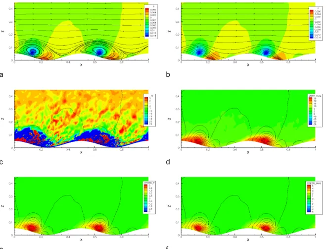
Figure 4.2: Examples of vortex identification using different criteria (streamlines, Q criterion, vorticity magnitude, cross-pressure gradient, magnitude of the pressure gradient

and pressure isobars) for case Re 150, phase t=0.25 s...60

Figure 4.3: Vorticity components and vorticity magnitude isosurfaces for case output_u064.

Cross-channel mean has not been substracted...61

Figure 4.4: Vorticity components and vorticity magnitude isosurfaces for case output_u064.

Cross-channel mean has not been substracted...62

Figure 4.5: Helicity density and relative helicity density isosurfaces for case output_u064.

Cross-channel mean not substacted...63

Figure 4.6: Helicity density and relative helicity density isosurfaces for case output_u064.

Cross-channel mean not substacted...63

Figure 5.1: Velocity profile evolution, averaged velocity evolution with phase, TKE profile

evolution and TKE average versus phase, case Re 42 ...64

Figure 5.2: Evolution of the velocity profile versus addimensional height in logarithmic scale,

case Re 42...65

Figure 5.3: Evolution of the longitudinal velocity contours with phase, (cross-channel,

10 cycle phase average) case Re 42...66

Figure 5.4: Evolution of the streamlines and pressure contours (phase and cross-channel

average,10 cycles) with phase, case Re 42...67

Figure 5.5: Evolution of the TKE contours (cross-channel, 10 cycle average) versus phase,

case Re 42...69

Figure 5.6: Cross-pressure gradient contours and pressure isobars (cross-channel, 10 cycle

average): evolution versus phase, Re 42...70

Figure 5.7: Pressure gradient magnitude contours and pressure isobars (cross-channel,

10 cycle average) evolution versus phase, Re 42...71

Figure 5.8: Vorticity magnitude contours (cross-channel, 10 cycle average) evolution versus

phase, Re 42...72

Figure 5.9: Q Criterion contours and pressure isobars (cross-channel, 10 cycle average) evolution versus phase, Re 42...73

Figure 5.10: Velocity profile evolution, averaged velocity evolution with phase, TKE profile

evolution and TKE average versus phase for case Re150...74

Figure 5.11: Evolution of the vertical velocity profile versus phase,

Figure 5.12: Pressure contours and streamlines for different phase values

(cross-channel, 10 cycle average), Re 150...76

Figure 5.13: TKE contours versus phase (cross-channel, 10 cycle average ), Re 150...78

Figure 5.14: Cross-pressure gradient contours and pressure isobars versus phase

(cross-channel, 10 cycle average ), Re 150...78

Figure 5.15: Pressure gradient magnitude contours and pressure isobars versus phase

(cross-channel, 10 cycle average ), Re 150...80

Figure 5.16: Vorticity magnitude contours and pressure isobars versus phase

(cross-channel, 10 cycle average ), Re 150...81

Figure 5.17: Q contours and pressure isobars versus phase

(cross-channel, 10 cycle average ), Re 150...82

Figure 5.18: Velocity vertical profile evolution, averaged longitudinal

velocity versus phase, TKE vertical profile evolution, and TKE average versus phase

(10 cycle average), Re 210...83

Figure 5.19: Evolution of the velocity vertical profile versus phase, logarithmic scale

(10 cycle average), Re 210...84

Figure 5.20: Longitudinal velocity contours versus phase

(cross-channel, 10 cycle average), Re 210...85

Figure 5.21: Pressure contours and streamlines versus phase

(cross-channel, 10 cycle average), Re 210 ...86

Figure 5.22: Pressure contours and streamlines

(cross-channel, 10 cycle average, t=3 s), Re 210...87

Figure 5.23: TKE contours versus phase

(cross-channel, 10 cycle average), Re 210 ...88

Figure 5.24: Cross-pressure gradient contours versus phase

(cross-channel, 10 cycle average), Re 210...89

Figure 5.25: Vorticity magnitude contours versus phase

(cross-channel, 10 cycle average), Re 210...90

Figure 5.26: Q contours versus phase

(cross-channel, 10 cycle average), Re 210...91

Figure 5.27: Evolution of the three-dimensional coherent structures field with time

(instantaneous field) using Q isosurfaces, Re 42...92

Figure 5.28: Comparison between cross-pressure gradient, pressure gradient magnitude, vorticity and Q isosurfaces for Re 42, t=0.167 s...94

Figure 5.30: Coherent structures' evolution as described by vorticity magnitude and Q isosurfaces, phase t=2-4 s, instantaneous field, Re 210...97

CHAPTER 0: INTRODUCTION

In the context of geophysical fluid dynamics, oscillatory flows in a boundary layer have important

implications in many ocean processes, such as sediment erosion, transport and deposition,

biogeochemical fluxes through the water-sediment interface, bedform morphogenesis and creation of

microbiotopes for benthic organisms. The flow dynamics due to the interaction between a wave field

and a mean, steady current over a wavy bottom is controlled in great part by the creation, advection

and dissipation of coherent structures, flow regions were important physical quantities such as velocity

or density have correlation scales larger than the smallest eddies. These coherent structures have a

direct impact in processes such as sediment pick up rates due to the generation of strongly localized (in

time and space) flow subdomains with high values of velocity perturbations, vorticity and Turbulent

Kinetic Energy (TKE).

The purpose of this thesis is to asses the effectiveness of several methods for the identification of such

structures in velocity and pressure fields computed using a Large Eddy Simulation (LES) numerical

scheme of a pressure driven oscillatory flow over a wavy bottom in a relatively wide range of Reynolds

number. I also will describe relevant physical characteristics of these flows elucidated using the spatial

and temporal distribution of such structures, and show that they can be used to distinguish between

several flow regimes as a function of the Reynolds number.

Chapter one deals with the description of the Large Eddy Simulation (LES) numerical scheme used in

the simulations. Chapter two describes the postprocessing subroutines developed by the author and

used to transform the output files into data readable by a Computer Fluid Dynamics (CFD) Visualization

package called TECPLOT©. Chapter three deals with a brief overview of coherent structures in

boundary layer flows and their importance in the Turbulent Kinetic Energy (TKE) generation, advection

instantaneous and averaged velocity and pressure fields and the methods used to identify coherent

structures in Chapter four. In Chapter five I describe the results of the application of these methods to

three flows with different Reynolds number. Finally, Chapter six gives a short summary of the most

CHAPTER 1: COMPUTATIONAL SETUP

SECTION 1.1: OVERVIEW

In order to study the properties of oscillatory and pulsating flows over a wavy bottom several numerical

experiments were performed with different values for the Reynolds number. Of these experiments,

three were selected for a detailed analysis using the postprocessing subroutines described below (case

Reynolds Number Re=42, Re=150 and Re=210). This Chapter describes the numerical scheme used in

the simulations and the flow domain.

SECTION 1.2: DESCRIPTION OF THE NUMERICAL SCHEME AND THE FLOW DOMAIN

A Large Eddy Simulation (LES) numerical scheme was used to calculate the flow properties for this

study. LES has been used successfully before for the elucidation of coherent structures, in

oceanographic and engineering flows, and there is abundant literature regarding its advantages over

other types of numerical schemes (Direct Numerical Simulation - DNS, Unsteady Reynolds Averaged

Navier Stokes - URANS, etcetera; see Tseng 2004, Balaras 2001, Piomelli 2000 and 2001, Chang

2004 and undated, Henn 1999, Fede undated, Tseng 2004). LES solves the filtered Navier-Stokes

equations:

1.1

u



i

,

t

 

u

i

u



j



,

j

=− 

P

i

 

u

i

,

ij

−

ij

,

j (overbar indicates an adequate average and comma denotes derivative;



is the kinematic viscosity) ; and the continuity equation

1.2

u



i

,

i

=

0

; the Subgrid Scale Stress (SGSS) is defined as 1.3



_ij

=

u

_i

u

_j

−

u

_i

u



j

explicitly. All spatial derivatives are approximated using second-order central differences. For further

details see Chang (undated).

Using the geophysical convention for the reference system, the domain is 0.1 m long (x1, longitudinal

axis), 0.1 m wide (x2, cross-channel or transversal axis) and 0.055 m high (x3, vertical axis). The grid

used in our simulations is an Arakawa-C (staggered) type with 288 (longitudinal direction) x 64

(cross-channel direction) x 128 (vertical direction) cells. The cell size is constant in the horizontal plane but

changes along the vertical to increase the grid resolution towards the upper and lower boundaries (see

figure 1.1). Boundary conditions are periodic in the longitudinal and cross-channel directions; at the

bottom we enforce a no-slip condition along an immersed boundary defined by a sinusoidal function:

1.4

z

_wall

=

_wall

∗[

1



cos



2

∗∗

x



_wall

]

z

wall being the bottom height,



_wall the ripple's amplitude and



_wall its wavelength.

At the upper surface the flow satisfies a no-slip condition along a plane wall. Although this disposition

does not resemble exactly the natural conditions in the ocean (in a wave-driven flow the upper

boundary is a free-surface instead of a rigid wall) it was chosen in order to compare the results of the

simulations with experiments performed in a flume. Far enough from the upper boundary the properties

of the flow do not differ significantly from those of a flow under a free surface for the set of parameters

chosen for our simulations (but see further comments about this assumption in Chapter 5).

The flow is driven by an periodic pressure gradient:

1.5

p



x ,t

=∇

p

0

∇

p

1

e

−ipt _;

∇

p

0 and

∇

p

1 being respectively the

magnitude of the steady and unsteady components of the pressure gradient and

T

=

2

_



p its

period. The Reynolds number is defined using an average velocity:

1.6

_R

_e

₌

U

0

∗

l

s



=

U

₀

∗





T



1.7

_U

0

=



_T

∗

∫

0

T

2

U



t

∂

t

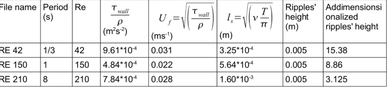
and ls is the thickness of the laminar oscillatory boundary layer (Stokes 1901). The relevant parameters

CHAPTER 2: DESCRIPTION OF THE POST-PROCESSING SUBROUTINES

SECTION 2.1 : OVERVIEW

The aim of this thesis is to study and identify coherent structures in oscillating and pulsating flows over

a wavy bottom using a visualization package named TECPLOT©. Unfortunately, the files generated by

the LES code can not be read directly by TECPLOT© so an intermediate step is necessary, namely, the

format conversion from the original data from the simulations to a file that can be understood by the

visualization program.

The simulation code generates a set of variables (in our case, the complete velocity and pressure

fields) from which other quantities useful for the identification of coherent structures can be calculated.

Although TECPLOT© has the capability to compute secondary or derived variables from this set, this

capability is limited: certain variables, like the second invariant of the velocity gradient tensor, must be

calculated by an external program prior to visualization (see reference TECPLOT© for a detailed

description of the visualization package). For reasons of convenience and practicality it is also easier to

generate other quantities, like averages and statistics, using external programs instead of TECPLOT©.

This section will describe the set of (crude) FORTRAN 95 subroutines I wrote in order to achieve this

double goal (format conversion and secondary variables' generation). The choice of programming

language was decided based on the desire to complement a similar set written by Dr. Pascal Fede in

2004. In retrospective, this was an unfortunate decision; using a higher-order programming language

SECTION 2.2 : DESCRIPTION OF THE SUBROUTINES

A typical output of the LES code consists in a group of files that constitute a temporal series depicting

the flow evolution over a certain time period (t1,t2). The number of files M is:

2.1 M = fs . c fs being the sampling frequency (in our case, 8 samples per period)

and c the number of cycles (for clarity sake, I will define a cycle as the time interval between the initial

phase Φ0 = 0 and the final phase Φ0 + T, T being the characteristic forcing period). Thus, each

consecutive file

2.2 FILE_NUMBER = 1, 2, 3, ..., 7, 8, ..., M-1, M ; corresponds with a time TLEVEL

TLEVEL = t0+Φ0, t0+Φ1, t0+Φ2, ..., t0+Φ7, t0+T, ..., t0+ (c-1)T + Φ7, t0+ (c-1)T + T

TLEVEL = t0, t0+Φ1, t0+Φ2, ..., t0+Φ7, t0+T, ..., t0+ (c-1)T + Φ7, t0+ c.T



₀

=

0

;



₁

=

T

f

s

;



₂

=

2T

f

s

;

...

;



₇

=

7T

f

s

For this study I have chosen c = 10 cycles, M = 80 files. Each file contains the full (3D) instantaneous

velocity [pressure] field for a given time (TLEVEL). The velocity [pressure] fields are written in the

format (using FORTRAN-like pseudocode):

do k=1,NZ

do n=1,3 [n=1,1] do j=1,NY do i=1,NX

un(i,j,k,TLEVEL) [ pn(i,j,k,TLEVEL)]

end do end do end do end do

NX, NY, NZ being the number of cells in the longitudinal, cross-channel and vertical direction

respectively and n the number of components for each variable (3 for the velocity vector, 1 for

pressure).

After running a simulation the postprocessing subroutines read these files and calculate the variables

listed in Table 2. The first variable computed by the subroutines is the instantaneous cross-channel

2.3

u

i

,

inst



x

1

, x

3

, t

=

_NY

1

∑

1

NY

u

i



x

1

, x

2

, x

3

, t



(the equation for pressure is

homologous)

Notice that the instantaneous cross-channel average for a given time is calculated using the velocity

[pressure] at that particular time (there is no further averaging either in time or phase). The

instantaneous perturbation velocity [pressure] is then calculated:

2.4

u '

i

,

inst



x

1

, x

2

, x

3

, t

=

u

i

,

inst



x

1

, x

2

, x

3

, t

−

u

i

,

inst



x

1

, x

3

,t



By definition, the cross-channel average of this variable is zero. All the other variables (Turbulent

Kinetic Energy – TKE -, vorticity, pressure gradient, etcetera) are subsequently computed using the

perturbation velocity [pressure]. All the derivatives are calculated using a second-order centered

differences scheme.

It is also possible to obtain phase-averaged quantities, which are useful in assessing the mean flow

characteristics during a "typical" cycle. Thus we define a averaged variable (for example,

phase-averaged pressure) as:

2.5

p



x

,



k

=

p



x

,t

=

k



p



x

, t

=

k



T





p



x

, t

=

_k



2T



...



p



x

, t

=

_k



c

−

1



T



p



x

,t

=

_k



c.T



p



x

,



_k

=

∑

m=0

c−1

p



x

,



_k



m . T



x = x1,x2x3 , Φ being the phase and c the number

of cycles.

Once the variables are calculated the postprocessing code outputs three sets of files: one containing

the full 3-D variables' field (usually named “RE#_3DFIELD_N.DAT”, N being a consecutive number); a

second containing the average of each variable in the cross-channel direction (usually named

“RE#_2DFIELD_N.DAT") and a third file containing the average of each variable in the flow domain

(excluding the space occupied by the ripples):

2.6

var

=

1

L

1

1

L

2

∑

i=1

NX

∑

j=1

NY



1

L

3k=

∑

kbottom NZ

L2, L3(x1), the length, width and depth of the channel (“TKE_AND_VEL_VS_PHASE.DAT”). All the files

are written in a TECPLOT© compatible format (again, expressed as FORTRAN pseudo-code):

TECPLOT HEADER (Contains information for TECPLOT©)

do k=1,NZ do j=1,NY do i=1,NX

xn (n=1:3), list of variables

end do end do end do

(Full 3-D output)

TECPLOT HEADER (Contains information for TECPLOT©)

do k=1,NZ do i=1,NX

xn (n=1,3) , list of variables

end do end do

(Output averaged in the cross-channel direction)

The value of the Cartesian coordinates xi is addimensionalized using the domain length.

Once the raw files have been processed, a program called PREPLOT© is used to transform the ASCII

files (extension *.dat or *.DAT) generated by the FORTRAN subroutines into binary files (extension

*.plt), which have the advantage of occupying less space. This is done automatically by executing a

UNIX script called scr_preplot also generated by the subroutines (once transformed the ASCII files into

TECPLOT© files, scr_preplot erases the files with extension *.dat .It is advisable to save the ASCII files

before executing scr_preplot).

The actual plots can be created either manually (a tedious process if involves more than a few files,

Thus, a typical post-processing sequence would be:

- Decide if we want a time series or a phase average from our original output files

- Compile and run the post-processing code

- Check the ASCII files for errors and save the *.dat files

- Run the script scr_preplot

CHAPTER 3: DEFINITION OF COHERENT STRUCTURES

This Chapter provides a brief introduction to the definition and description of coherent structures in

boundary layer flows. This topic has been the subject of much attention and a fair number of literature

due to its importance in the context of turbulent flows, so in the interest of brevity I will give just a

general idea of the most important concepts and remit the interested reader to the relevant references

for the necessary details.

For the purpose of this study I will define a coherent structure as a flow region over which one or more

fundamental variables (velocity, density, energy, etcetera) has a significant correlation with itself or with

other variables over a range of space and/or time significantly larger than the smallest local scales of

the flow (Robinson 1991). Although this definition does not require any kind of vortical motion, in

practice most coherent structures do posses a certain degree of rotation.

Coherent structures have been observed in a large variety of experiments and simulations of

geophysical and engineering flows (Carlier 2005, Tufo 1999, Blondeaux 2004, Cantwell 1981, Chang

undated, Marchioli 2006, Nakagawa 2003, Robinson 1991, Scotti 2001, Tseng 2004). Their importance

lays in several factors:

- In many flows, they control the generation and dissipation of turbulent kinetic energy. The

early models of TKE transfer in turbulent flows assume a direct energy transfer from the larger scales

(large, energy containing, eddies) to the smallest wavelengths (Kolmogorov scales). The formation of

coherent structures introduces an additional step, transferring energy from small scales (infinitesimal

perturbations) to the intermediate scales characteristic of such structures (Robinson 1991, Natrajan

not constant with time, but changes in a quasiperiodic fashion. This so called intermittency problem has

been related to the generation and evolution of coherent structures (Robinson 1991).

- In a more practical way, coherent structures introduce inhomogeneities in the spatial and

temporal distribution of Reynolds stresses and perturbation velocity correlations. It has been suggested

that this variability has a direct impact in the geochemical fluxes in the interface between sediment and

water column (and between air and water in the ocean surface). Bottom stress controls the sediment

uptake in sandy environments; vortical structures can increase the time spent by sand grains in the

water column, with the corresponding change in erosive, transport and deposition fluxes (an important

consideration in studies of coastal and beach environments, with engineering applications such as

beach nourishment, channel dredging, navigational hazards, etcetera) (Dronkers 2005).

Coherent structures are generated by instabilities in the turbulent flow (either primary or secondary)

such as shear instabilities, Görtler instabilities (Reed 1989, Swearingen 1987), perturbations of wakes

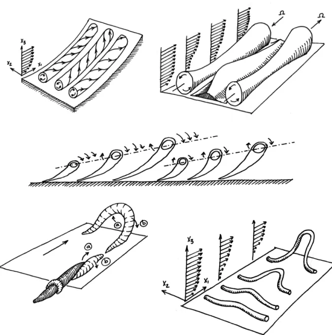
and separation layers (Delery 2001), etcetera. Such structures usually assume the shape of rolls or

filaments, which tend to interact between themselves in complex ways. Some examples of structures

commonly observed in sheared flows are:

- Sweeps and bursts: sweeps are structures that carry fluid with high momentum downwards

from the outer zone to the viscous/buffer region (u'1>0, u'3<0), while bursts transfer low-momentum fluid

upwards from the bottom (u'1<0, u'3>0). They act as an enhanced momentum and mass diffusion

coefficient.

- Low velocity streaks are longitudinally oriented, cigar-shaped structures possessing a lower

velocity than their surrounding fluid. They seem to be related to flow patterns in the inner side of

counter-rotating vortices, although several other mechanisms have been suggested (Chernyshenko

2005, Jimenez 1988).

- Horseshoes, arches, hairpins and lambda vortices are filament-like structures generated by a

secondary instability in cross-channel rolls. They are lifted from the bottom due to the interaction

between their own vorticity and the vertical velocity gradient in the mean flow; the same gradient

then dissipate into the background flow (see figure 3.1 ; Robinson 1991).

CHAPTER 4: VORTEX IDENTIFICATION METHODS

SECTION 4.1: OVERVIEW

This chapter will provide a description of several vortex identification methods that can be used in the

elucidation of coherent structures in oscillatory flows over ripples. It is not intended by any means as an

exhaustive enumeration but just as a review of the multiple approaches that can be used in order to

tackle this problem, and a discussion of their advantages and disadvantages. Only a few of those

procedures were actually used by the author in the study of the LES simulations, but I think it is useful

to provide the reader with at least an introduction to the methodologies considered, and their

advantages and disadvantages, in order to better understand why and when those criteria can be

applied with confidence.

Section 4.2 provides the reader with a working definition of vortices in the context of instantaneous and

averaged fields. Section 4.3 is an enumeration of the different available methods. Section 4.4 describes

the application of the velocity field and the streamlines to the problem of vortex identification. Section

4.5 describes winding angle and quadrant methods. Section 4.6 deals with vorticity, helicity density and

relative helicity. Section 4.7 is a summary of the pressure minimum criterion and, finally, the Q criterion

will be dealt with in Section 4.8.

SECTION 4.2: DEFINITION OF VORTICES AND COHERENT STRUCTURES IN INSTANTANEOUS

AND TIME-AVERAGED FIELDS

The concept of vorticity and vortex is very useful in the context of turbulent motion. The properties of

a framework of interconnected vortex filaments (Jeong 1995). Unfortunately, one major obstacle for the

understanding of turbulent processes is the lack of an accepted definition of what constitutes a vortex

although there is a certain consensus about the important properties that the concept should include.

These are the following:

- From a kinematic point of view, in a vortex material particles of the fluid rotate around a

common center or core (Jeong 1995).

- The structure has net vorticity (thus excluding potential – irrotational - vortices); the definition

of a vortex should be Galilean invariant, meaning that it remains unchanged under transformations of

the form:

4.1

y

=

Qx



a

t

where Q is an orthogonal tensor and a is a constant velocity

vector (Jeong 1995 ; Haller 2005 in his attempt to improve upon Jeong's definition proposes a stronger

condition called objectivity, defined as the invariance under coordinate changes of the form:

4.2

y

=

Q



t



x



b



t



where Q(t) is a time-dependent orthogonal tensor and b(t) is a

time-dependent translation vector).

- The particle rotation implies the presence of a centrifugal force that must be balanced against

either a pressure gradient, a friction force, a change in the flow velocity or a combination of these

factors. If the temporal scale of the motion is large and the effects of friction are small enough the core

of a vortex can be characterized by a local minimum in the pressure field (Jeong 1995).

Many criteria have been postulated that satisfy one or more of these properties (Banks undated, Dubieff

2000, Guo 2004, Jeong 1995, Jiang undated, Moffat 1992, Stegmaier 2005, Tufo 1999). The

applicability of a given criterion to a particular case depends on the approach taken in the identification

scheme: either kinematic (with a focus in the description of the motion without considering the forces

that act on the fluid particles) or dynamic (which concerns itself with those forces) and, of course, with

the specific characteristics of the process. (For a more detailed discussion on the properties of a vortex

see Jeong 1995 and Haller 2005).

that actual fluid particles rotate around a core. But from a statistical point of view no scientific and

reliable inferences about a certain phenomenon can be made from just one experimental realization.

Statistical certainty demands a set of experiments, under similar enough conditions and parameters, in

order to extract from said set the properties that characterize that particular kind of fluid motion. Thus

we define an ensemble average as the mean of a series of realizations of a given flow, undertaken

under conditions that do not differ enough as to change significantly the results of such experiments

(Kundu 1990).

Ensemble averages are of course a physical utopia that can be extremely hard to achieve in the real

world, specially in observational oceanography where the operational and logistic difficulties and the

rarity of some phenomena make this scientific ideal many times an unattainable goal. Even in the case

of computer simulations running multiple iterations of a single experiment can be very expensive and

time consuming. I will consider then, for the purpose of this study, a phase average (defined elsewhere

in this document) as a reasonable proxy under the assumption that the flow is ergodic in the sense of

Blackman 1959 (namely, that a short sample is representative of the whole process).

The extension of the definition of a vortex from the instantaneous case to the averaged flow is not

straightforward and we must proceed with caution. Two ways are open in front of us: the first one is to

try to relate the characteristics of the averaged flow to the structures from which they originate as

observed in the instantaneous velocity field. Incidentally this is the way Leonardo da Vinci identified

coherent structures in a river flow as described by Holmes 1996 and Marani 2003. In his observations

of water moving around an obstacle, Leonardo realized that certain discrete vortices are consistently

located roughly in the same place and have approximately the same size, and inferred that the motion

can be decomposed into a mean component and a series of “undulations” (coherent structures). The

disadvantage inherent in this approach is that it defeats the purpose of an average, namely, obtaining a

characterization of the flow properties from a sum of its realizations, not from the detailed study of each

and single one of a series of snapshots .

of both) and then define a coherent structure as a subdomain of the averaged flow which partakes from

the characteristics ascribed to a vortical structure in the non-averaged case (namely, a region in the

domain where the average velocity, pressure, etcetera, correlate at a larger scale than the smallest

eddies in the flow). In the context of a vortical description of a turbulent flow then we can expect that the

attributes of coherent structures in non-averaged flows (high vorticity, rotation around a core, pressure

minima) describe also adequately these structures in the averaged case. Notice that the definition of

coherent structures in the averaged case is fundamentally different from that in the non-averaged case.

In the latter, vortices are constituted by real fluid particles with a rotational motion while in the former the

structures are born from the averaged flow characteristics, implying larger time and space correlation

scales. The pitfall in this approach is that we could fall into the danger of identifying as vortices

structures born out of the averaging operation which bear distant or no relation with the actual physical

processes happening in the flow, or that real, physical vortices will be obscured or even eliminated in

the mean variable field. Both approaches have their merits and drawbacks and I will use one or the

other depending on the particular problem we are faced with.

In order to provide a clarifying example (although using a spatial, not temporal, average), consider a

field of longitudinally-oriented counter-rotating vortices. It is obvious that we can not use, for example,

the cross-channel average of the longitudinal component of the vorticity to identify these particular

vortices in a channel cross section, although this quantity is a good descriptor in a three-dimensional

instantaneous field. In the other hand, intrinsically positive quantities such as vorticity magnitude are

immune to this particular kind of problem. Of course, more subtle problems arise in the process of

averaging operations, many of which have no obvious solution and compromises must be made.

SECTION 4.3: CRITERIA FOR DETECTION AND QUANTIFICATION OF VORTICAL COHERENT

STRUCTURES

As explained above, the lack of an accepted definition of a vortex translates in a multitude of criteria

detect coherent structures is closely related to two considerations: first, how much operator input we

want or we are able to provide and, second, the intrinsic properties of the given flow. This section will

provide a general overview of several methods currently used in the elucidation of coherent structures,

namely:

- Methods using the velocity field and streamlines

- Winding angle and quadrant methods

- Vorticity and vorticity magnitude methods

- Helicity density and Relative Helicity

- Pressure minima

- Eigenvalues of the velocity gradient tensor: Q criterion

SECTION 4.4 VELOCITY FIELD AND STREAMLINES METHODS

A simple, kinematic approach to vortex detection is the study of the actual velocity field (either plotting

the velocity vector or using streamlines) in order to identify visually the regions where the flow has a

circular pattern. This method has a long tradition, especially in the field of experimental hydro- and

aero-dynamics, and this is the reason for the existence of an abundant literature on the subject (for a

discussion and many illustrations of the use of streamlines and streaklines, see Batchelor 1967 or Dyke

1982). It has the advantage of being fairly intuitive and it can be very useful in moderately complex 2D

flows, or if we are concerned with averaged quantities; it is a very effective way of visualizing a

recirculation zone. In 3D flows its usefulness is very limited except in the simplest motions. A further

disadvantage of this method is that it is not Galilean invariant, as can be readily seen in figure 4.2, a-b.

SECTION 4.5 WINDING ANGLE AND QUADRANT METHODS

These are intrinsically kinematic methods that focus in the circular motion of the fluid particles in a

vortex and, as is the case with streamlines, do not fulfill the condition of being Galilean invariant. The

- The winding angle of the streamlines in a vortical structure must have a value close to 2π.

- The distance between the projection of the initial and the ending points of the streamlines on a

2-D surface normal to the vortex core should be small (Guo 2004).

A related criterion is the quadrant or cross method. This method divides the plane normal to the core

into four (or more) sections with the origin located in the vortex center. If the origin is indeed a vortex

core, the circular pattern of the streamlines implies that they will cross the quadrants' axes in a certain

order.

Notice that these methods are based in the presumption that fluid particles surrounding a vortex core

undergo almost one complete revolution in the time scale characteristic of the motion. A vortex with a

rotation period longer than the advective time scale of the flow, or that it is being stretched by a shear

motion, will not be detected. These methods are also unable to detect structures undergoing pairing or

breakdown processes, and have also the disadvantage of depending upon a correct projection of the

three-dimensional streamlines into a plane normal to the suspected vortex core (Jeong 1995).

SECTION 4.6: VORTICITY, HELICITY DENSITY AND RELATIVE HELICITY

The definition of a vortex, as stated by Jeong 1995, explicitly demands the existence of net vorticity

(excluding potential or irrotational vortices). This is a necessary but not sufficient condition: for example,

the boundary layer over an infinite plate (Blasius flow) has net vorticity but no vortices; thus caution

must be exerted using vorticity as an indicator for the presence of coherent structures.

Vorticity is defined as the antisymmetric part of the velocity gradient tensor:

4.3 ω i =εijk(uk)j εijk being the permutation operator

εijk = 0, if any two of i,j,k are the same

1, if ijk is an even permutation of 1,2,3

-1, if ijk is an odd permutation of 1,2,3 (Aris 1962)

Galilean invariance.

A related flow property is the helicity density which is a pseudo scalar (meaning that it changes sign

under parity transformation - a change in the coordinate system defined as a mirror reflection of the

axis):

4.4 h = ui ω i

It measures how much the fluid swirls or corkscrews in a helicoidal fashion. If we integrate the helicity

density over a domain D in a three dimensional Euclidean space we obtain the helicity:

4.5 H = ∫D ui ω i dV

An important property of helicity is that it is a conserved quantity if the evolution of the flow is governed

by the Euler equations (a condition not satisfied by boundary layer flows due to the effects of viscous

stress; for more details see Moffatt 1992).

Another related flow property is the relative helicity density defined as:

4.6

h

_rel

=



u

i



i



∣

u

∣∗

∣



∣



The relative helicity density is the cosine of the angle between the velocity vector and the vorticity.

Helicity and relative helicity could be useful in the elucidation of vortices with a strong advective

component in the direction parallel to their axis. In the other hand, one disadvantage of both helicity

density and relative helicity density is the inability to distinguish between a slow moving flow with strong

rotational component and a fast moving fluid with weak rotation.

The fact that relative helicity density provides only the angle between a vortex and the flow but does not

measure its strength also works against its use for identification purposes, as it can be seen in Figure

4.5 b and Figure 4.6 b. The relative helicity density field is unable to distinguish between the relatively

strong, slowly advected, vortices at the bottom and the weaker vortices in the upper, faster zone of the

A problem that arises with vorticity and vorticity-related quantities as pointed out in Jeong 1995 and

Haller 2005 is that in many cases background vorticity obscures the presence of smaller scale vortices

in a flow, a concern which strongly applies in our case. A possible way of removing this undesired

background is to define a de-meaned velocity field u'i (and analogously a de-meaned pressure field p')

by substracting the cross-channel velocity (pressure) average from the original field:

4.7

u '

i

=

u

i

−

u

i ;

u

i defined as

u

i



x

1

, x

3

, t

=

1

L

_2x

∫

2=y0

L2

u



x

_i

,t

∂

x

₂

4.8

p'

=

p

−

p

;

p

defined as

p



x

1

, x

3

, t

=

_L

1

2x

∫

2=y0

L2

p



x

i

,t

 ∂

x

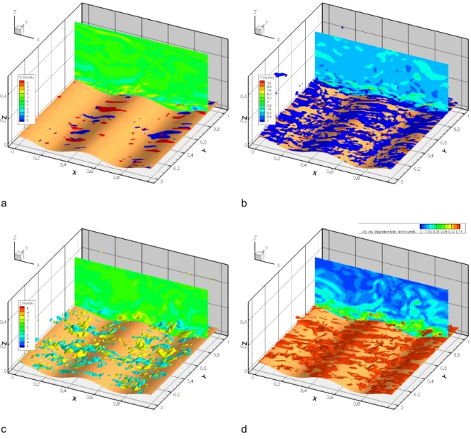
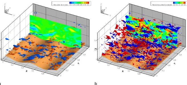
2 L2 being the

channel width. The effects of this operation are depicted in Figures 4.3, 4.4, 4.5 and 4.6 for the case of

a shear flow over a wavy bottom with constant speed. The first two plots show the three components of

the vorticity and the vorticity magnitude, while the following plots show the helicity density and relative

helicity density fields for the same flow.

With reference to the vorticity, the biggest differences arise in the cross-channel component and the

vorticity magnitude. The delicate filaments noticeable in the de-meaned fields are obscured in the

original flow by the signal from the strong vertical velocity shear. Less affected is the vertical component

although the simple de-meaning is able to extract more detail than the original data. Finally, the

longitudinal component shows few (if any) differences.

A similar behavior is observed in the second set of figures. The number of structures shown in the

de-meaned helicity field is greater than in the original data and their shape is more elongated. Finally,

although the change is difficult to perceive, a similar tendency is observed in the relative helicity field.

SECTION 4.7 LOCAL PRESSURE MINIMA

Assuming a cyclostrophic equilibrium, in a rotational or swirling motion the centrifugal force due to the

be characterized by a pressure minimum surrounded by a region with a relatively strong pressure

gradient which can be used as identification methods. This minimum can exist in all three directions or

only in a plane normal to the vortex axis (as for example is the case of the Burgers vortex) (Jeong

1995). Thus we can define the pressure gradient magnitude along the three spatial axes:

4.9

∣∇

p

∣=



∑

i=1 3



∇

p



i

2

or we can define the pressure gradient only in a plane normal

to the longitudinal direction x1:

4.10

_∣∇

_p

_∣

_cross

₌



∑

i=2 3



∇

p



i

2

which I will call cross-channel pressure gradient

magnitude.

Of course a strict cyclostrophyc equilibrium is only possible in a steady, inviscid planar flow

(incidentally, not the case of pulsating boundary layer flows over ripples, which violates all of the three

restrictions) and the effectiveness of this elucidation method will be inversely proportional to the degree

the flow departs from these three conditions.

We must also take into account the fact that vortices can exist as a result of processes not involving

pressure effects whatsoever. A classical example is the von Kármán viscous pump in which a vortex is

generated by a rotating disc immersed in a fluid as a result of a balance between viscous and

centrifugal forces, the pressure variation in the radial direction being identically zero.

An example of the results using this method is shown in figure 4.2 e-f. Pressure contours are plotted as

SECTION 4.8: Q CRITERION

This criterion is named after the second invariant of the velocity gradient tensor:

4.9

Q

=

1

2



ij



ij

−

S

ij

S

ij



where



_ij

=



u

i

,

j

−

u

j

,

i



2

and

S

ij

=



u

_i

,

_j



u

_j

,

_i



2

are respectively its antisymmetric and

symmetric parts. Thus in regions where the rotation rate, given by



_ij , overcomes the strain rate,

given by

S

_ij ,

Q

has a positive value. The relation between

Q

, vorticity magnitude and pressure is:

4.10

Q

=

1

4

∣∣

2

−

2

S

_ij

S

_ij

=

1



2



p ,

ii

The value of

Q

is then proportional to the Laplacian of pressure. Although in practice it is usually the case, notice that if inside a given domain

Q

is positive that does not necessarily imply a local minimum for pressure inside the domain (as a consequence of the minimum principle, the lowest

pressure values could be located in the border); there is no exact correspondence between the

Q

criterion and the pressure criterion (for a more detailed discussion see Dubieff 2000, Jeong 1995).

The

Q

criterion is Galilean invariant but some caveats must be considered before using this method to identify vortices. First and more important we must decide what value to use as a threshold. If the

value is too small, any location where even a feeble amount of rotation can overcome and even smaller

strain will be considered a potential vortex and the spurious signals could obscure the physically

relevant structures; in the other hand, if the value is too restrictive we risk missing those same relevant

structures.

Another problem is that

Q

is not an absolute measure of the vortex strength, but of the strength in relation to the flow strain. Thus a strong vortical structure undergoing stretching can give a signal

partially overcome if we know roughly where the regions with strong shear are located, although in

CHAPTER 5: ELUCIDATION OF COHERENT STRUCTURES IN PULSATING AND OSCILLATORY

FLOWS

SECTION 5.1: VERTICAL GRADIENT SIGNAL IN A BOUNDARY LAYER FLOW

As explained above (see Chapter 3), if we are interested in the smaller scales of the process as

opposed to the mean background flow it is desirable to separate this long wavelength signal from the

original field. Considering the system geometry and the fact that our flow is characterized by a strong

vertical shear a natural way to accomplish this is to substract the cross-channel mean from the

three-dimensional velocity (pressure) field and define a new perturbation variable:

5.1

v

i



x

1,

x

2

, x

3

, t

=

v '

i



x

1,

x

2

, x

3

, t



v

i



x

1

, x

3

, t



p



x

1,

x

2

, x

3

, t

=

p'



x

1,

x

2

, x

3

, t



p



x

1

, x

3

, t



where the bar denotes a

variable averaged in the cross-channel (x2) direction and the prime a de-averaged velocity. But which

channel average?. Two immediate choices are available: either the phase average of the

cross-channel mean:

5.2



v

i



x

1

, x

3

,



k

=

∑

n=0

c−1



1

L

₂



_x

∫

2=0

L2

v

_i



x

₁

, x

₂

, x

₃

,t

₀



_k



nT

∂

x

₂

(and an analogous expression for pressure), Φk being the phase, c the number of cycles, L2 the

channel width and T the period; k in this formula does not relate to the index in the vertical direction.

Notice that this average is a function of the phase but not of time. Or the second choice, the

instantaneous cross-channel mean:

5.3



v

i



x

1

, x

3

, t

=



1

L

₂



_x

∫

2=0

L2

v

_i



x

₁

, x

₂

, x

₃

, t

∂

x

₂ which is a function of time.

v



x

i

,t

−

v



x

1,

x

3

=

O



l



(same with pressure); then the second average will give the variability

of the processes at small scale Ψs while the first average will give the variability of the interactions

between the processes at small and large scale.

Due to the fact that the results obtained using the instantaneous cross-channel average have a simpler

physical interpretation than those using the phase average of the cross-channel mean I have decided to

use always the first average to calculate the value of the perturbation velocity and pressure for the

purposes of this study.

SECTION 5.2 : THE EFFECT OF SPATIAL AND TEMPORAL RESOLUTION IN THE

IDENTIFICATION OF COHERENT STRUCTURES

The characteristic time scale of turbulent fluctuations in a steady flow over a flat bottom is a function of

the flow characteristics such as TKE, energy dissipation rate ε and local velocity gradient (Chen 2003).

In an oscillatory flow, additional time and space scales appear as the oscillation period T and the

ripples' characteristic length scale λ which affect the evolution and spatial distribution of such structures.

Let us assume that the smallest dimension in a vortex is given by a certain wavelength λc , and that we

can define a characteristic time scale Tc (which can be understood either as an advective or local

period, borrowing terminology from the Navier-Stokes equations). Clearly, in order to detect the vortical

signal the grid resolution must be greater than the length scale λc :

5.4



_c



_crit

=

2



l

_grid where lgrid is the maximum cell size and λcrit represents the

threshold value; and in a similar way:

5.5

f

s



f

crit

=

1



2

T

c



fs being our sampling frequency (Blackman 1959)

In practice, some of the mathematical operations in the postprocessing code act as a de facto low pass

The difficulty in an unsteady case lays thus not only in verifying this condition for the intrinsic time and

space scales of the structures, but we must also take into account that their generation, advection and

dissipation is constricted by the external time and space scales of the mean flow. This problem will be

discussed in more detail for each particular case.

SECTION 5.3: TEST CASES FOR THE ELUCIDATION OF COHERENT STRUCTURES

Although the topic of this thesis is vortex identification procedures, it is helpful to acquire at least a basic

knowledge of the evolution of the flows where these schemes are being applied. As described in more

detail in Chapter 3, all of these methods work under assumptions related to the characteristics of the

structures under investigation; the effectiveness of the criteria is a function of the motion unsteadiness,

mean flow deviation from planarity, spatial and temporal distribution of high shear zones, etcetera.

Knowing when and where the flow departs from these assumptions is helpful in the assessment of the

applicability of every method to a particular problem and allow us to predict, not only what works and

what does not, but why, when and where a scheme works or does not.

The three flows considered are pressure-driven boundary layer flows in a channel over a wavy bottom.

The flow parameters are described elsewhere in this document (see Chapter 1 and table 1). Both cases

Re=42 and Re=210 are pulsating flows with a period of T42 = 1/3 s and T210 = 8 s respectively (pulsating

meaning that the average of the longitudinal velocity u1 over the flow domain, although changing with

time, is always positive) while the case Re=150 is an oscillating flow with a period T150 = 1 s (oscillating

implies a reversal of the averaged longitudinal velocity). The cases discussed here were chosen in

order to assess the detection of structures in flows with different Reynolds number.

SECTION 5.4 : FLOW DESCRIPTION, CASE REYNOLDS 42

The evolution of the phase-averaged longitudinal velocity ui and the similarly averaged TKE for case Re

amplitude 0.086 m s-1 _{and period T}

42 = 1/3 s; it reaches its peak at phase t=0 s and its minimum value

at t=0.17 s. Velocity has been adimensionalized using the friction velocity:

5.1 U+ ₌

v

u

_f uf being the friction velocity

u

f

=







₀





and τ0 the shear stress at the

bottom. Similarly, the vertical dimension is given in terms of wall units:

5.2 y+ ₌

_u

f

x

3





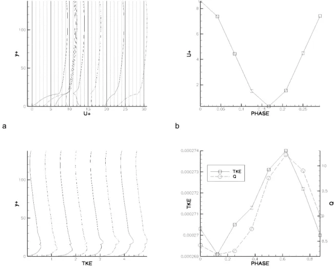
being the kinematic viscosity (Kundu 1990).

As shown in Figure 5.1-5.2 the vertical shear in the outer region of the boundary layer (roughly from

y+_{=30 to y}+_{= 100) remains approximately constant with time. The shear in the viscous and buffer layers} *

is not constant: its (positive) value decreases from the maximum at phase t=0 s (which corresponds

with the velocity maximum) to t=0.083 s. At some point between t=0.083 s and 0.125 s past the middle

point in the deceleration stage the shear changes its sign and increases its magnitude until reaching a

maximum at t=0.17 s. A further sign reversal (this time from negative to positive) happens between

t=0.21 s and 0.25 s at the beginning of the acceleration stage, shortly after the velocity minimum;

afterwards the shear grows again to achieve its peak at phase t=0 s.

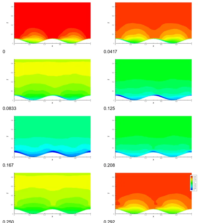
The phase- and cross-channel-averaged longitudinal velocity field U1 is depicted in Figure 5.3. Notice

how mass conservation lifts the isotachs (equal velocity contours) over the troughs. The velocity

variations in the outer region (upper half of the domain) are of the order of 0.15 ms-1 _{which is half the}

magnitude of the velocity change in regions near the bottom (ΔU1~0.3ms-1), specifically those on top of

the crests. The downstream side of the crests is also a zone with high vertical shear from the phase

t=0.29 s to t=0.042 s, while strong vertical gradients are apparent along most part of the ripples from

t=0.125 to t=0.17 s; at t=0.208 s these are concentrated on the crests.

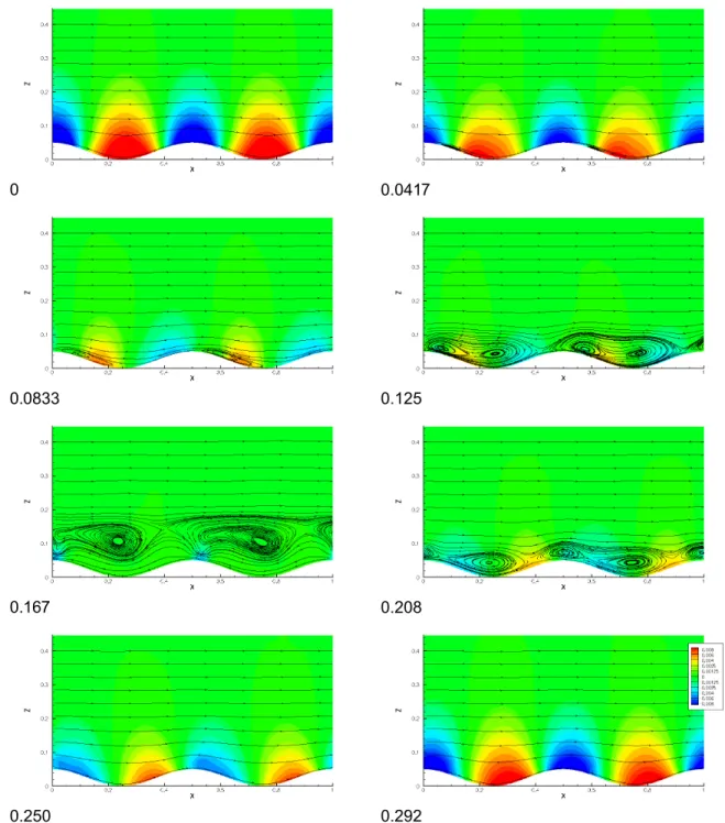
Directing our attention to the phase- and cross-channel-averaged pressure and streamlines field, we

can infer from figure 5.4 the existence of two stages in the flow evolution from a kinematic point of

view. The first stage spans from phase t=0.250 s to t=0 s (the end of the acceleration phase as shown

in figure 5.1), roughly 40% of the flow period, and is characterized by the fact that the streamlines follow

the bottom profile. The second stage lasts from t=0.042 s to t=0.21 s. At the beginning of this second

stage the flow deceleration induces a recirculation zone in the downstream side of the ripples

(t=0.042-0.083). Just before the velocity minimum the recirculation vortex deattaches from the bottom and a

second vortex is created above the troughs. The lifting process reaches its maximum height at t=0.167

s and a strong recirculation flow develops immediately above the bottom; after that, the mean flow

acceleration “pushes down” the vortices until at t=0.25 s those have completely disappeared. The effect

of the mean flow vortices is a local increase of the vertical shear in certain zones of the ripples,

specially on the recirculation zone and in the region near the crests from t=0.125 s to t=0.208 s. This

shear generation will be noticed in the second invariant of the velocity gradient field (see further

comments below). These vortices are accompanied by saddle points (critical points that are stable in

one direction and unstable in the other) which indicate regions where the flow suffers stretching and

compression, processes that can hinder the detection of coherent structures.

Another important flow characteristic which I would like to address is the evolution of the

phase-averaged TKE, as depicted in figure 5.1, c-d. The variation of the TKE in this flow is very small (less

than 2%) and it is concentrated mostly in the lower part of the domain, around the maximum ripple

elevation (in non-dimensional height units, y+_{=15.88). There is a phase displacement of ΔΦ=1.25π}

radians between the velocity and the TKE (meaning that the TKE reaches its maximum about 0.04 s

after the velocity minimum and the TKE minimum occurs an equal time delay after the velocity peak).

The phase- and cross-channel-averaged TKE spatial distribution for each phase is shown in figure 5.5.

We can distinguish two regions roughly corresponding with generation and dissipation processes,

although the separation is not complete. The first is the upper part of the ripples, which is mainly a

generation region. Creation of TKE starts at t=0.042 s (beginning of the deceleration stage) at the

upstream side of the ripples; by t=0.125 s there are two maxima on the crests, one a bit downstream

and a second located just below the crest vortex. The regions merge at t=0.17 s just before the TKE

crests seem to expand in space. Notice that the generation and growth of the TKE patch located on the

crests spans almost a complete period. After t=0.293 s the patch is advected by the background flow

and moves rightwards towards the troughs. At first glance it seems to engulf a preexistent “blob” located

at the upstream side of the ripples (t=0.042 s) and then dissipate until at t=0.25 s (again, almost a

complete period after the beginning of the dissipation phase) only a weak patch of fossil TKE remains.

But this evolution is not consistent with the rapid increase shown in Figure 5.1 from t=0.0833-0.125 s,

which is difficult to ascribe to the crest structures. The answer lies in the longitudinal velocity variability

field (U1MS, not shown), which shows a generation episode from t=0.042 s to t=0.083 s located at the

ripples' troughs, slightly above the recirculation zone.

SECTION 5.5 : IDENTIFICATION OF COHERENT STRUCTURES, CASE REYNOLDS 42

In this section I will describe the structures identified using the pressure field, cross-channel pressure

gradient magnitude (cross pressure gradient for short), pressure gradient magnitude, vorticity

magnitude and Q criterion. Due to the slowly evolving nature of this particular flow I will only discuss the

observations for phase t=0, 0.083, 0.167 and 0.25 s. Instead of depicting the pressure field in a

separate plot I have decided to show the contour lines as the background for all the other variables,

with the added advantage of making comparisons between criteria more easy.

As shown in Figure 5.6-5.9 and specially in Figure 5.4 the large scale variations in the phase- and

cross-channel-averaged pressure correspond roughly with coarse changes in the phase-averaged

mean velocity field (lower pressure on crests and higher in troughs related to respectively faster and

slower mean flow, with lateral excursions in the contours due to the oscillations in time). A closer look at

the contours (more evident in Figure 4.6) reveals that the pressure field does delineate, albeit in a

slanted form, departures from the background flow. Thus the recirculation zones (t=0.083 s, compare to

the streamlines plot, Figure 5.4) show as indentations of the isobars; and the shear zone above the

The phase- and cross-channel-averaged cross pressure gradient and pressure gradient magnitude

fields confirm the information given by the pressure field and point towards the existence of new

structures. As shown in Figures 5.6 and 5.7, the recirculation zone signal (t=0.083 s) is associated with

maximum values of these variables evident in both plots (see also Figure 111) and the maxima

observed on the crests at t=0.17 s can also be related to the patterns observed in the mean flow (strong

streamline curvature and deceleration-acceleration of the counterflow); notice also the correspondence

between the indentations and loops in the pressure field and the pressure gradient contours. But three

new structures arise at t=0, 0.083 and 0.25 s which can not be related to the mean flow as described by

the streamlines.

At t=0 s we observe peaks in the distribution of both quantities (although weaker in the case of the

cross pressure gradient magnitude) at the downstream side of the ripples and in one of the crests. At

t=0.083 s a new structure arises over the troughs (although barely discernible in the cross pressure

signal) and again at t=0.25 s a strong signal is evident on the crests seemingly uncorrelated to the

background flow. Notice that these structures do relate to deformations of the averaged pressure field.

The phase- and cross-channel-averaged vorticity magnitude and Q fields (Figure 5.8 and 5.9) confirm

and qualify the picture obtained by the other criteria, but also point to the existence of a richer structure

field. The examination of the vorticity magnitude contours (Figure 5.8) indicates that the structures

described by the pressure criteria have a strong rotational component, but it also shows that its spatial

distribution does not completely correlate with the aforementioned vortices. At phases t=0, 0.083 and

0.17 s the vorticity spans a substantial portion of the ripples downstream region, although the first two

examples could be partially explained by the formation of the recirculation zone.

The Q field explains part of this discrepancy. The regions with high vorticity and low pressure gradient

show also low Q values, which indicates the existence of high shear values (thus negating the

precondition of cyclostrophy). Notice also that, although we have a close match between the pressure

gradients do. From the fact that the trough vortices also show (relatively) high values of vorticity, we can

infer that this is due to the existence of high shear which impedes the pressure field from achieving a

condition of equilibrium.

An observation with reference to the relation between the phase- and cross-channel-averaged TKE and

vortex detection criteria must be made. Until now, no consideration has been given to the dynamical

processes that generate and destroy vortical coherent structures; as shown above, it is perfectly

possible to design a purely kinematic vortex detection criterion. But numerous experiments and

simulations correlate the existence of these structures with elevated values of TKE, and it is almost

certain that vortices do play an important role in the creation, transport and dissipation of TKE. In our

case, a comparison between the TKE contours (Figure 5.5) and Q values (Figure 5.9) shows that there

is indeed a strong correspondence between the two; specially in the case of the trough regions (which

are mainly dissipative zones), where high TKE correlates with elevated vorticity and low shear. The

relation is a bit more complex on the crests (notice that the relatively high values of TKE upstream of

the ripples at t=0.083 s do not show in the Q field; neither high Q values downstream the ripples show

in the TKE contours); this can be due to the fact that at this stage of the flow TKE is being created by a

strong shear without an adjacent generation of vorticity (but do notice that this is almost the only

exception in the whole period; at any other time we can readily relate all TKE with corresponding Q

structures).

The relation between Q values and TKE is also quite evident after looking at Figure 5.10, which shows

the evolution of both variables with phase (the evolution of the other variables also shows a certain

dependence with TKE, but none of them tracks the energy as closely as Q). The Q method thus has the

advantage of serving not only as a vortex identification criterion but also as a good predictor of the

evolution in time and distribution in space of the TKE.

In summary: the temporal evolution of case Re_42 shows a laminar-like stage and a period