ANALYZING SAMPLING IN STOCHASTIC OPTIMIZATION: IMPORTANCE SAMPLING AND STATISTICAL INFERENCE
Yang Yu
A dissertation submitted to the faculty of the University of North Carolina at Chapel Hill in partial fulfillment of the requirements for the degree of Doctor of Philosophy in the
Department of Statistics and Operations Research.
Chapel Hill 2019
Approved by: Amarjit Budhiraja Shu Lu
Sayan Banerjee
c
○ 2019 Yang Yu
ABSTRACT
YANG YU: ANALYZING SAMPLING IN STOCHASTIC OPTIMIZATION: IMPORTANCE SAMPLING AND STATISTICAL INFERENCE.
(Under the direction of Amarjit Budhiraja and Shu Lu.)
The objective function of a stochastic optimization problem usually involves an expec-tation of random variables which cannot be calculated directly. When this is the case, a common approach is to replace the expectation with a sample average approximation. How-ever, sometimes there are difficulties in using such a sample average approximation to achieve certain goals. This dissertation studies two specific problems.
In the first problem, we aim to solve a minimization problem whose objective function is the probability of an undesired rare event. To accurately estimate this rare event proba-bility by Monte Carlo simulation, an extremely large sample is required, which is expensive to implement. An importance sampling scheme based on the theory of large deviations is developed to efficiently reduce the sample size and thus reduce the computational cost. The convergence of a sequence of approximation problems is also studied, through which a good initial point to the minimization problem can be found. We also study the buffered proba-bility of exceedance as an alternative risk measure instead of the ordinary probaproba-bility. Under conditions, the analogous minimization problem can be formulated into a convex problem.
ACKNOWLEDGMENTS
This is the last part I wrote in my dissertation and this is also the most difficult part. There are many people who have earned my gratitude for their contribution to my life.
First and foremost I must thank my advisors Professors Amarjit Budhiraja and Shu Lu, for supporting me during these past five years. This work would not have been possible without their tremendous guidance and involvement. Under their guidance, I learned how to accurately define a research problem and find a solution to it. I am also grateful to the excellent examples they have set as successful researchers. Besides research, I also appreciate the valuable advices from Professor Shu Lu on my teaching work and also my life.
I would like to thank the rest of my dissertation committee members Professors Quoc Tran-Dinh, Mariana Olvera-Cravioto and Sayan Banerjee for taking the time out of their busy schedule to read this dissertation and provide feedbacks. I am grateful to Professor Quoc Tran-Dinh for his suggestions on my research and LaTeX tricks for making equations better look. Also, I would like to thank Alison Kieber, Christine Keat and Samantha Radel for taking care all the administrative work.
Next, I would like to give special thanks to Professors Daniel Ocone and Shadi Tahvildar-Zadeh of the Mathematics Department at Rutgers University. It was Professor Daniel Ocone’s class inspired my curiosity about stochastic calculus (although my research is not in this) and made me think about applying for a Ph.D. program. As a student with Finance major, I was far from being confident to start my application for a math related Ph.D. program. During that time, Professor Shadi Tahvildar-Zadeh placed a lot of trust and confidence in my abilities which encouraged me to click the submit button.
support.
Last but not the least, I would like to thank my family for all their love and encouragement. For my parents Zhenan and Jing who supported me in all my pursuits both emotionally and financially. I would never be able to pay back their love and the sacrifices they made in raising me. And most of all for my supportive and patient husband Shuo. He is always dependable and steady in the past nine years. I would not have made it here without him. Thanks also go to my parents in-law Zhanquan and Yujie for their support and accepting me into the family as one of their own.
TABLE OF CONTENTS
LIST OF TABLES . . . ix
LIST OF FIGURES . . . xi
1 Introduction . . . 1
1.1 Minimization of rare event probabilities . . . 1
1.2 Inference of two-stage stochastic linear programming problems . . . 3
2 Minimization of a class of rare event probabilities . . . 5
2.1 Introduction . . . 5
2.2 Large deviation based importance sampling schemes . . . 6
2.2.1 Basic importance sampling scheme . . . 6
2.2.2 Background on the theory of large deviations . . . 7
2.3 Two importance sampling schemes . . . 9
2.3.1 The exponential change of measure on variables Ui . . . 10
2.3.2 The exponential change of measure on variables Xi . . . 14
2.4 Convergence of approximate problems . . . 25
2.5 Minimization of the buffered failure probability. . . 32
2.6 Computational experiments . . . 34
2.6.1 Reformulation and solution of the limiting problem . . . 35
2.6.2 Implementing importance sampling in the gradient method . . . 36
2.6.3 Computation on minimization of the buffered probability . . . 39
3 Inference of two-stage stochastic linear programming . . . 48
3.1 Introduction . . . 48
3.2 Background . . . 50
3.3 Asymptotic behavior of the normal map solution . . . 53
3.4 Estimation of LnorK and Σ0 . . . 63
3.5 Confidence regions and confidence intervals . . . 71
3.5.1 Nonsingular covariance matrices . . . 71
3.5.2 Singular covariance matrices . . . 81
3.6 Numerical experiments . . . 84
3.6.1 An R2 example with a nonsingular Σ0 . . . 86
3.6.2 An R10 example with a nonsingular Σ0. . . 90
3.6.3 An R100 example with a nonsingular Σ0 . . . 91
3.6.4 An R2 example with a singular Σ0 . . . 93
3.6.5 Coverage rates of confidence intervals/regions with perturbed covari-ance matrices . . . 96
4 Conclusion . . . 98
LIST OF TABLES
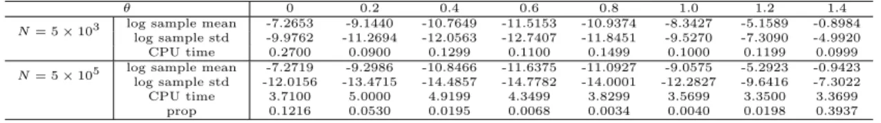
2.1 Estimation of p(θ) using ordinary Monte Carlo simulation in Example 1 . . . 40 2.2 Estimation of p(θ) with the change of measure on Ui in Example 1 . . . 40 2.3 Estimation of p(θ) with the change measure on Xi in Example 1 . . . 41 2.4 Lower and upper bounds of the decay rate with importance sampling scheme
in Section 2.3.2 for Example 1 . . . 42 2.5 Parameters in Example 2 . . . 43
3.1 Coverage rates (%) of the 95% confidence region forz0 calculated with estima-tors/true values . . . 88 3.2 Coverage rates (%) of the 95% individual confidence intervals forz0 withα1 =
α2 = 0.025, n= 2 and a nonsingular Σ0 . . . 88 3.3 Coverage rates (%) of the 95% individual confidence intervals forz0 calculated
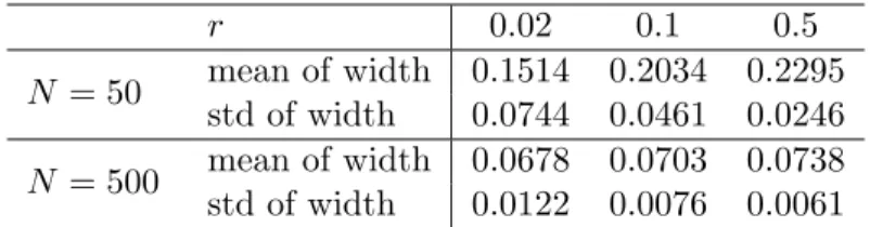
with estimators/true values,α1=α2 = 0.025 . . . 89 3.4 Widths of the confidence intervals for (z0)1 with α1 =α2 = 0.025, n= 2 and
a nonsingular Σ0 . . . 89 3.5 Summary of O2fM,N(ˆxN) for different support radius withN = 500 . . . 90 3.6 Summary of O2fM,N(ˆxN) for differentN withr= 0.02 . . . 90 3.7 Coverage rates (%) of the 95% confidence region for z0 with n = 10 and a
nonsingular Σ0 . . . 91 3.8 Coverage rates (%) of the 95% individual confidence intervals forz0 withα1 =
α2 = 0.025, n= 10 and a nonsingular Σ0 . . . 92 3.9 Coverage rates (%) of the 95% individual confidence intervals forz0 withα1 =
α2 = 0.025, n= 100 and a nonsingular Σ0 . . . 93 3.10 Coverage rates (%) of 95% individual confidence intervals for z0 with n = 2
and a singular Σ0 . . . 95 3.11 Coverage rates (%) of 95% individual confidence intervals for x0 with n = 2
LIST OF FIGURES
2.1 Trajectories of objective values of (2.60) in the gradient method for Example 1 with ordinary Monte-Carlo simulation . . . 42 2.2 Trajectories of objective values of (2.60) in the gradient method for Example
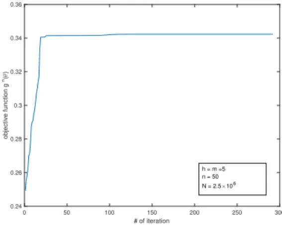
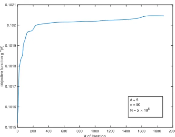
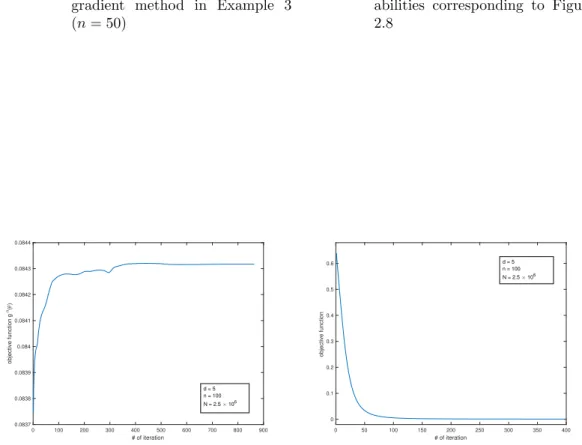
1 with the IS scheme from Section 2.3.2 . . . 42 2.3 Objective values of (2.60) for the gradient method in Example 1 . . . 43 2.4 Objective values of (2.60) for the gradient method in Example 2 (h= 2) . . . 44 2.5 The contour map ofgnclose to the optimal solution in Example 2 (h= 2) . . 44 2.6 Objective values of (2.60) for the gradient method in Example 2 (h= 5) . . . 45 2.7 Objective values of (2.60) for the gradient method in Example 3 (n= 50) . . 46 2.8 Objective values of (2.58) for the gradient method in Example 3 (n= 50) . . 47 2.9 Probabilities and buffered probabilities corresponding to Figure 2.8 . . . 47 2.10 Objective values of (2.60) for the gradient method in Example 3 (n= 100) . 47 2.11 Objective values of (2.58) for the gradient method in Example 3 (n= 100) . 47
CHAPTER 1: Introduction
The sample average approximation (SAA) method is a basic approach to estimate the expectation in the objective function of a stochastic optimization problem. However, some-times there are difficulties in using such an SAA to achieve certain goals. In this dissertation, we mainly focus on two specific problems. In the first problem, the sample average from the Monte Carlo simulation is every inefficient in estimating the expectation. In the second prob-lem, the SAA function is not as smooth as the expectation function and thus does not provide enough information to compute confidence intervals of the solution. These two problems are studied in Chapter 2 and Chapter 3 separately. Notations of Chapter 2 and Chapter 3 are independent. In the remaining of this chapter, we give overviews of Chapter 2 and Chapter 3.
1.1 Minimization of rare event probabilities
In Chapter 2, we consider a stochastic optimization problem of the form
min θ∈ΘP
" 1
n
n X
i=1
G(Xi, θ)∈A #
where Θ is a subset in Rd, G(x, θ) is a continuous function from Rh ×Θ to Rm and Xi,
i= 1, . . . , n, are independent and identically distributed (i.i.d.) Rh-valued random variables.
identify the appropriate Issacs equations whose subsolutions are used to construct importance sampling schemes with the change of measure on the distribution ofXi. In Section 2.3, we detailedly discuss how to construct such a scheme and prove the asymptotic results. In the same section, the importance sampling scheme in [12] is also briefly summarized. Comparing to the scheme in [12], the replacement measure of our scheme is more tractable and thus a sample of realizations from the replacement measure is easy to generate. By implementing such techniques, we can estimate the objective function accurately with a relatively small sample. Another difficulty in solving such a minimization problem is to figure out an initial point. In general, the objective function not need to be convex, if we start the minimization algorithm from a randomly chosen initial point, the algorithm may terminate at a local minimum far away from the global minimum. We handle this problem by studying the convergence of a sequence of approximation problems to the original problem in Section 2.4. These convergence results guarantee that we can use the solution of the limiting problem as an initial point when solving a fixed approximation problem whose solution is close to the solution of the original problem.
When the value of the functionG(x, θ) is a scalar, the buffered probability of exceedance can be used as an alternative measurement of risk instead of the ordinary probability. Some related results in [5] are included in Section 2.5 which show that the importance sampling schemes that are asymptotically efficient for the ordinary probability are also asymptotically efficient for estimating the buffered probability of exceedance. Under certain conditions, the buffered probability of exceedance is a convex function of the parameterθthus finding a good initial point is no longer a problem.
1.2 Inference of two-stage stochastic linear programming problems
In the second part, we focus on a two-stage stochastic linear programming problem which has the following form:
min x∈Rn
cTx+E[Q(x, ξ)]
s.t. Ax=b, x≥0,
(1.1)
whereQ(x, ξ) is the optimal value of the second-stage problem:
min y∈Rm
qTy
s.t. V x+W y=h, y≥0.
(1.2)
Here ξ := (q, h, V, W) are the input data of the second-stage problem and some or all of the elements can be random. Our goal is to construct confidence intervals/regions for the solution of (1.1). Since a two-stage stochastic programming problem can be written as a stochastic variational inequality (SVI), a natural idea is to implement methods designed to compute confidence intervals for an SVI solution, see [20, 21, 23, 24, 25]. In those methods, an SVI is first written into a normal map formulation and the confidence intervals are based on the asymptotic results of the normal map solution. We first review some background knowledge about the normal map formulation, piecewise affine functions and the B-derivative in Section 3.2. Then in Section 3.3, we define normal map solutions for problem (1.1) and the corresponding SAA problem, and prove the required asymptotic results.
The difficulty in computing confidence intervals/regions is to estimate the Hessian of the objective function in (1.1) at the solution. This is because a sample average approximation of the objective function is piecewise linear when it is finite. Accordingly the Hessian of the sample average function is zero when it exists. To deal with this difficulty, we smooth the piecewise linear sample average function by a convolution with a kernel function. Justification of this approach and implementation are included in Section 3.4.
CHAPTER 2: Minimization of a class of rare event probabilities
2.1 Introduction
We consider a stochastic optimization problem with the following setting. Let Θ be a subset in Rd,G(x, θ) be a continuous function from Rh×Θ to Rm and Xi,i= 1, . . . , n, are i.i.d random variables with values inRh. We study the following problem
min θ∈ΘP
" 1
n
n X
i=1
G(Xi, θ)∈A #
(2.1)
whereA is a measurable subset ofRm. When the value ofθ is considered as fixed, we define
random variables Ui :=G(Xi, θ) andYn:= n1 Pni=1Ui for simplicity. In many applications in engineering, finance, and insurance, decisions need to be made to reduce the probability for an undesirable event (such as system breakdown) to occur. Such an event is often the result of the accumulative effects of a large number of individual events over a long period, which we model as{Yn∈A}, withnbeing a fixed large number. And we refer to (2.1) as a fixed-n problem.
The objective function in (2.1) is not convex in general and its values in many problems of interest are extremely small and thus hard to estimate. These characteristics of the prob-lem require us to address two main issues: estimating the objective function efficiently and choosing the initial point wisely. The second difficulty can be handled by solving the limiting problem which is defined in Section 2.4, while the first difficulty is solved by a importance sampling scheme based on the large deviation theory.
if the necessary and sufficient conditions for effective variance reduction in [6, 39, 40] are violated. Later papers then develop adaptive schemes to make this technique more generally applicable. Among these papers, Dupuis and Wang’s works [11, 12] are most related to our work. The paper [11] connects the problem of constructing asymptotically efficient adaptive (feedback) importance sampling schemes with certain deterministic dynamic games. The second paper [12] uses subsolutions to the Isaacs equations associated with such games to construct flexible and simple dynamic importance sampling schemes that achieves asymptotic efficiency. In both of these papers, the importance sampling scheme is based on exponential twists of the laws of the summandsUi which can be non-standard and intractable and thus computationally demanding. Our method is based on the exponential twists of distributions ofXi which take a simpler form than those forUi, so a sample form the replacement measure ofXi is easy to generate especially when Xi are from the exponential family.
When Ui take values in R, the buffered probability of exceedance as an alternative risk
measure instead of the ordinary probability. The buffered probability of exceedance was introduced in Rockafellar and Royset [35] and its mathematical and statistical properties are studied in [26, 27]. When the function G and the Θ satisfy certain conditions, the optimization problem with the buffered probability of exceedance as its objective function is convex, thus the initial point can be arbitrary. The importance sampling schemes which are asymptotically efficient for the ordinary probability are also asymptotically efficient for estimating the buffered probability of exceedance as shown in [5].
2.2 Large deviation based importance sampling schemes
2.2.1 Basic importance sampling scheme
The probability in (2.1) can be written asE[1{Yn∈A}] where 1{y∈A}is the indicator function
that takes value one when y ∈ A and zero otherwise. For this section and Section 2.2.2, suppose thatYnhas density functionp(y). Let ¯Ynbe a random variable with density function
q(y) such thatp(y)dy is absolutely continuous with respect toq(y)dy. Then
E[1{Y ∈A}] =E
1{Y¯ ∈A}p( ¯Yn)
If the density functionq is chosen carefully such that
E
"
1{Y¯n∈A} p( ¯Yn)
q( ¯Yn) 2#
<E[1{Yn∈A}],
the importance sampling estimate
1
k
k X
i=1 1{Y¯i
n∈A}
p( ¯Yni)
q( ¯Yi n)
, Y¯ni ∼Y¯n i.i.d.
toE[1{Yn∈A}] is ”more efficient” than a sample average of i.i.d. copies 1{Yn∈A}. The bound
on the best possible performance (as measured by the second moment) can be obtained by Jensen’s inequality
E
"
1{Y¯n∈A} p( ¯Yn)
q( ¯Yn) 2#
≥
E
1{Y¯n∈A} p( ¯Yn)
q( ¯Yn) 2
= E[1{Yn∈A}]
2
. (2.2)
E[1{Yn∈A}] is the unknown value of interest, so the above inequality does not provide any
practical guidance in finding the best density functionq. However, the theory of large devia-tions describes the asymptotic behavior ofE[1{Yn∈A}] based on which asymptotically efficient
importance sampling schemes can be developed.
2.2.2 Background on the theory of large deviations
In this section, we briefly introduce some fundamental results in the theory of large devia-tions which describes the asymptotic behavior of the remote tails of a sequence of probability distributions. The material of this section is mainly taken from [4].
Definition 2.1(Rate function). A functionImappingRminto[0,∞]is called a rate function
if for each M <∞ the level set {x:I(x)≤M} is a compact subset of Rm.
Definition 2.2 (Large deviation principle (LDP)). Let {Yn} be a sequence of Rm-valued
random variables and letI be a rate function on Rm. We say that the sequence {Yn} satisfies
(i) For every open subset O of Rm
lim inf n→∞
1
nlogP[Yn∈O]≥ −yinf∈OI(x).
(ii) For every closed subset C of Rm
lim inf n→∞
1
nlogP[Yn∈C]≤ −yinf∈CI(x).
Roughly speaking, a large deviation principle gives the exponential decay rate of the probabilities asP[Yn∈A]≈exp{−ninfy∈AI(y)}. Suppose that the sequence of probabilities
{P[Yn ∈ A]} have a decay rate governed by a LDP, given as infy∈AI(y) = γ. Then, the following inequality follows from (2.2)
−lim inf n→∞
1
nlogE
"
1{Y¯n∈A}p( ¯Yn)
q( ¯Yn) 2#
≤ −lim inf n→∞
2
nlog (P[Yn∈A]) = 2γ.
An importance sampling scheme is said to be asymptotically efficient if the above inequality also holds for the other direction, that is,
−lim inf n→∞
1
nlogE
"
1{Y¯n∈A}p( ¯Yn)
q( ¯Yn) 2#
≥2γ.
The Cram´er’s theorem and the Sanov’s theorem are two basic results in the large deviations theory. Both of them concern the most basic setting of averages of i.i.d. random variables, but from different point of views. The Cram´er’s theorem gives the LDP for the empirical mean of i.i.d. random variables, while the Sanov’s theorem considers the empirical measure. Theorem 2.1 (Cram´er’s theorem). Let {Un} be a sequence of i.i.d. Rm-valued random
variables with common distributionξ, and letYn= 1n
Pn
i=1Ui. Assume that
R
ehu,viξ(du)<∞
for everyv∈Rm. Then the sequence {Y
n} satisfies the LDP with rate function
I(u) = sup v∈Rm
hu, vi −log Z
ehu,viξ(du)
.
entropy of the probability measure ν with respect to ξ, defined as
R(νkξ) = Z
Rm logdν
dξdν (2.3)
whenν is absolutely continuous with respect to ξ and ∞ otherwise.
Theorem 2.2 (Sanov’s theorem). Let {Un} be a sequence of i.i.d. Rm-valued random
vari-ables with common distributionξ, and letLn be the empirical measure of the firstnvariables:
Ln(du) = 1
n
n X
i=1
δUi(du).
Then{Ln} satisfies the LDP on P(Rm) with rate function I(ν) =R(νkξ).
2.3 Two importance sampling schemes
In this section, we consider the estimation of
Eexp{−nF(Yn)} (2.4)
whereF is a measurable function fromRm toR∪ {+∞}. It is useful to note that if F takes
also obtained using the large deviations theory.
First, we define the following functions which are useful when formulating the partial differential equations in both approaches. For (a, α)∈Rh+m, we define
H(a, α) = logE
h
eha,X1i+hα,G(X1)ii. (2.5)
We then define functionsH1:Rh →Rand H2 :Rm→R as
H1(a) =H(a,0), a∈Rh (2.6)
and
H2(α) =H(0, α), α∈Rm. (2.7)
Note thatH1 is the log-moment generating function ofX1 and H2 is that ofU1=G(X1).
2.3.1 The exponential change of measure on variables Ui
We briefly review the approach in Dupuis and Wang [12]. Within this subsection, we assume that H2(α) <∞ for all α ∈ Rm. Let ¯U1n, . . . ,U¯nn be the replacements of U1, . . . , Un under the new measure whose (conditional) distributions have the following form
ehα,ui−H2(α)ξ(du).
Recall that ξ is the distribution of U1. If α is a constant, then ( ¯U1n, . . . ,U¯nn) are i.i.d.. In general,α can be a function of space and time and we will discuss the general case later in this subsection. Based on ¯U1n, . . . ,U¯nn, a replacement of Yn is ¯Yn = n1
Pn
i=1U¯in. Then an unbiased estimator ofEexp{−nF(Yn)} is
Zn=. e−nF( ¯Yn)
n Y
i=1
eH2(α)−hα,U¯ini
where Qni=1eH2(α)−hα,U¯ini is the Radon-Nikodym derivative of the joint distribution of ( ¯Un
min-imization of the second moment of Zn and using the idea of dynamic programming, one is led to a partial differential equation whose solutions lead to a good choice ofα. That partial differential equation is called the Isaacs equation and is given as following. Let L2 be the Legendre transform ofH2, defined as
L2(β) = sup α∈Rm
[hα, βi −H2(α)], β ∈Rm.
Define function H2 :R3m →R∪ ∞as
H2(s;α, β) =hs, βi+L2(β) +hα, βi −H2(α).
The Isaacs equation is given as
Wt(y, t) + sup α∈Rm
inf β∈RmH2
(DW(y, t);α, β) = 0 (2.8)
whereW :Rm×[0,1]→R is a continuously differentiable function,Wt(y, t) is its derivative
w.r.t. t, and DW(y, t) is its derivative w.r.t. y. It turns out that a good subsolution to the Isaacs equation is often sufficient for constructing a good importance sampling scheme. In [12], they introduce a notion of generalized subsolution/control, which is very convenient for constructing importance sampling schemes.
Definition 2.3 (Generalized subsolution/control). Given K ∈ N, consider function W¯ :
Rm×[0,1] → R, ρk : Rm×[0,1] → R, α¯k : Rm×[0,1] → Rm, 1 ≤ k ≤ K, such that the
following properties hold. For all(y, t)∈Rm×[0,1], {ρ
k} satisfies ρk ≥0 and
K X
k=1
ρk(y, t) = 1.
¯
Wt and DW¯ can be written as
¯
Wt(y, t) = K X
k=1
DW¯(y, t) = K X
i=1
ρk(y, t)sk(y, t).
For each k= 1, . . . , K,
rk(y, t) + inf
β H(sk(y, t); ¯αk(y, t), β)≥0. (2.9)
The functions (rk, sk, ρk,α¯k)are uniformly bounded and Lipschitz continuous. The collection
( ¯W , ρk,α¯k) is called a generalized subsolution/control to the Isaacs equation (2.8).
In the above definition, the constant α in defining the exponential twist is replaced by a collection of functions {α¯k}k=1,...,K. With a generalized subsolution/control ( ¯W , ρk,α¯k), a dynamic change of measure can be constructed as follows. Let ¯Y0n= 0 and define
¯
Yjn= 1
n
j X
i=1 ¯
Uin. (2.10)
Since the parameter of the Radon-Nikodym derivative is replaced by a set of functions, there can exist dependency between ¯Uj+1n and all the ¯Ujn withl≤j and randomization in choice of
k∈ {1, . . . , K}. Now we introduce a randomized implementation of the importance sampling scheme based on ( ¯W , ρk,α¯k). At time j, we first generate a multinomial random variable I such that P[I = k] = ρk( ¯Yjn, j/n) for k ∈ {1,2, . . . , K}. Next, we simulate ¯Uj+1n from the distribution
ehα¯I( ¯Yjn,j/n),ui−H2( ¯αI( ¯Yjn,j/n))ξ(du). (2.11)
Then an unbiased estimator of Eexp{−nF(Yn)} is
Zn=. e−nF( ¯Ynn)
n−1 Y
j=0 "K
X
k=1
ρk( ¯Yjn, j/n)ehα¯k( ¯Yjn,j/n),U¯jni−H2( ¯αk( ¯Yjn,j/n))
#−1
.
When the terminal condition ¯W(y,1)≤2F(y) is satisfied for all y ∈Rm, [12, Theorem 8.1] provides an asymptotic lower bound of the logarithm of the second moment which is
lim inf n→∞ −
1
nlogE[(Z
Under regularity conditions onF , one has the large deviation principle
γ = lim n→∞−
1
nlogEexp{−nF(Yn)}. (2.13)
The Jensen’s inequality implies that−1
nlogE[(Z
n)2] is bounded by
¯
W(0,0)≤lim inf n→∞ −
1
nlogE[(Z
n)2] ≤lim sup n→∞
−1
nlogE[(Z
n)2]≤2γ.
The corresponding importance sampling scheme is asymptotically efficient if ¯W(0,0) is equal to the optimal decay rate 2γ.
In general, the distribution of Ui = G(Xi) may not take a simple form. Then for each
j, constructing a realization of ¯Ujn is expensive. We use a simple example to illustrate this. SupposeK = 1 andm= 2. At step j+ 1, ¯Uj+1n follows the distribution
ehα( ¯¯ Yjn,j/n),yi−H2( ¯α( ¯Yjn,j/n))ξ(dy).
Denote ¯Uj+1n as ¯Uj+1n =
¯
Uj+1n(1),U¯j+1n(2)
, the cumulative distribution function of ¯Uj+1n(1)as ¯FU¯n(1)
j+1 , and the conditional cumulative distribution function of ¯Uj+1n(2) given ¯Uj+1n(1)as ¯F¯
Ujn+1(2)|U¯n(1)
j+1
. Even if ξ has a closed form, finding ¯F¯
Ujn+1(1) and ¯FU¯jn+1(2)|U¯n(1)
j+1
might involve numerical integrations. When there is no closed form for those cumulative distribution functions, to generate a re-alization of ¯Uj+1n , first we generate two independent realizations e1 and e2 from the uniform distribution on [0,1]. A realizationu1 of ¯Uj+1n(1) and a realizationu2 of ¯Uj+1n(2) are the solutions to the following equations
¯
F¯
Ujn+1(1)(u1) =e1 ¯
F¯
Ujn+1(2)|U¯n(1)
j+1
(u1, u2) =e2.
2.3.2 The exponential change of measure on variables Xi
Motivated by the difficulty discussed above, we consider an importance sampling scheme by the change of measure onRh-valued random variables Xi, whose distribution is denoted asη.
In this subsection, we assume that H(a, α) <∞ for all (a, α) ∈Rh+m, and let L be the Legendre transformation ofH:
L(b, β) = sup (a,α)∈Rh+m
ha, bi+hα, βi −H(a, α)
, (b, β)∈Rh+m. (2.14)
ThenL has the following representation by [10, Lemma 6.2.3]:
L(b, β) = inf µ∈P(Rh)
R(µkη) : Z
Rh
xµ(dx) =b,
Z
Rh
G(x)µ(dx) =β
, (2.15)
whereP(Rh) denotes the space of all probability measures onRh and R(µkη) is the relative
entropy of the probability measure µwith respect toη.
In this importance sampling scheme, X1, . . . , Xn are replaced by the random variables ¯
X1, . . . ,X¯n which follow the distribution ηa defined as
ηa(dx) =eha,xi−H1(a)η(dx), (2.16)
wherea∈Rh.
In general, the constant a can also be chosen adaptively as a function of the spatial and time positions. Define that function as ¯a:Rm×[0,1]→Rh. Let ¯Y0n= ¯X0n= 0. At stepj+ 1, the random variable ¯Xj+1n follows the distributionηa( ¯¯Yn
j,j/n). Recursively define ¯Y
n j+1 as
¯
Yj+1n = ¯Yjn+G( ¯Xj+1n )/n.
Then an unbiased estimator of Eexp{−nF(Yn)} is
Zn=e−nF( ¯Ynn)
n−1 Y
j=0
The main advantage of this scheme compared to the scheme in Section 2.3.1 is that the function G does not affect the form of the new measure. Thus, random variables following
η¯a( ¯Yn
j,j/n) can be easily simulated even if the function G is complex. For example, if η is
a multivariate normal distribution with covariance matrix Σ, η¯a is also multivariate normal with the same covariance matrix Σ, but its mean is shifted by Σ¯a.
Recall that the large deviation principle for {Yn} and the Jensen’s inequality imply that
lim sup n→∞
−1
nlogE(Z
n)2 ≤2γ.
If we can construct a lower bound for lim infn→∞−1nlogE(Zn)2 and push this lower bound
close to 2γ by choosing a good function ¯a, then this importance sampling scheme is nearly asymptotic efficient. To find such a lower bound, we follow the process as in [12] to an Issacs equation associated with minimizing the second moment ofZn.
For each i= 0, . . . , n−1 and eachy ∈Rm, we set ¯Yn
i =y and define a quantityVn(y, i) as
Vn(y, i) = inf ¯ a E
e−nF( ¯Y
n
n)
n−1 Y
j=i
eH1(¯a( ¯Yjn,j/n))−ha( ¯¯ Yjn,j/n),X¯jn+1i
2
(2.18)
where the expectation is taken with respect to random variables ¯Xi+1n , . . . ,X¯nn,Y¯i+1n , . . . ,Y¯nn, and the minimization is taken over all the possible function ¯a. We also define Vn(y, n) = exp{−2nF(y)}. Note thatVn(0,0) is the minimum second moment ofZnthat can be achieved by this importance sampling scheme. Vn(y, i) can be written in the following form with the original measure, i.e., as an expectation ofXn
i+1, . . . , Xnn, Yi+1n , . . . , Ynn
Vn(y, i) = inf ¯ a E
e−n2F(Y
n
n)
n−1 Y
j=i
eH1(¯a(Yjn,j/n))−h¯a(Yjn,j/n),Xnj+1i = inf ¯ a E E e
−n2F(Yn
n)
n−1 Y
j=i+1
eH1(¯a(Yjn,j/n))−h¯a(Yjn,j/n),Xjn+1ieH1(¯a(y,i/n))−ha(y,i/n),X¯ ni+1i|Xn i+1 = inf ¯ a Z Rh
eH1(¯a(y,i/n))−h¯a(y,i/n),xiVn(y+G(x)/n, i+ 1)η(dx) = inf
a∈Rh Z
Rh
where Yin = y. The last equality holds because in infa¯ R
Rhe
H1(¯a(y,i/n))−h¯a(y,i/n),xiVn(y +
G(x)/n, i+ 1)η(dx), the minimization only optimizes the function ¯a at point (y, i/n) which is equivalent to minimizing a constantaoverRh. Next, defineWn(y, i) =−1nlogVn(y, i) for
each y∈Rm and i= 0,· · · , n. Fori < n we can writeWn(y, i) as
Wn(y, i) =−1
nlogV
n(y, i) =−1
nlog infa∈Rh
Z
Rh
eH1(a)−ha,xi+logVn(y+G(x)/n,i+1)η(dx) =−1
nainf∈Rh log
Z
Rh
eH1(a)−ha,xi−nWn(y+G(x)/n,i+1)η(dx).
From the Donsker-Varadhan relative entropy formula (see e.g. [10, Proposition 1.4.2], [12, Lemma 7.1]) we have
Wn(y, i) = sup
a∈Rh inf µ∈P(Rh)
1
n
R(µkη)−H1(a)+ Z
Rh
ha, xiµ(dx)
+ Z
Rh
Wn(y+G(x)/n, i+ 1)µ(dx)
.
(2.19)
LetW :Rm×[0,1]→Rbe a continuous function such thatWn(y, i) =W(y, i/n). Applying
the Taylor expansion onW(y+G(x)/n,(i+ 1)/n), we have
Z
Rh
W(y+G(x)/n, i+ 1)ν(dx)
≈W(y, i/n) + 1
nWt(y, i/n) +
1
n
Z
Rd
hDW(y, i/n), G(x)iν(dx),
where Wt and DW are the derivatives of W with respect to t and y respectively. We can then rewrite (2.19) in terms ofW as:
0 = sup a∈Rh
inf µ∈P(Rh)
R(µkη)−H1(a) + Z
Rh
ha, xiµ(dx) +Wt(y, t) + Z
Rh
hDW(y, t), G(x)iµ(dx)
Using the representation (2.15), the above equation can be rewritten as
sup a∈Rh
inf
(b,β)∈Rh+m[L(b, β)−H1(a) +ha, bi+Wt(y, t) +hDW(y, t), βi] = 0.
We defineH:R2m+2h →R∪ {∞} as
H(s, a, b, β) =ha, bi+hs, βi+L(b, β)−H1(a), s, β∈Rm, a, b∈Rh, (2.20)
and obtain the following Issacs equation
Wt(y, t) + sup a∈Rh
inf
(b,β)∈Rh+mH(DW(y, t), a, b, β) = 0, (2.21)
with the terminal condition W(y,1) = 2F(y).
Based on the Issacs equation, a generalized subsolution/control ( ¯W , ρk,¯ak) to (2.21) can be defined according to Definition 2.3 except that (2.9) is replaced by
rk(y, t) + inf (b,β)∈Rh+m
H(sk(y, t); ¯ak(y, t), b, β)≥0. (2.22)
For the special case in which K = 1 and ρ1 = 1, we abbreviate the notation ( ¯W , ρk,¯ak) as ( ¯W ,¯a) and call it a subsolution/control pair.
Through the same procedure of a dynamic change of measure based on ( ¯W , ρk,¯ak) as in Section 2.3.1, an unbiased estimator of Eexp{−nF(Yn)} can be constructed as follows. Let
¯
Y0n= 0 and define ¯Yj+1n = ¯Yjn+1nG( ¯Xin). At timej, we first generate a multinomial random variableI such that P[I =k] =ρk( ¯Yjn, j/n) for k∈ {1,2, . . . , K}. Second, we simulate ¯Xj+1n from the distribution
eh¯aI( ¯Yjn,j/n),xi−H1(¯aI( ¯Yjn,j/n))η(dx). (2.23)
Finally, we define
Zn=e−nF( ¯Ynn)
n−1 Y
j=0 " K
X
k=1
ρk( ¯Yjn, j/n)e
ha¯k( ¯Yjn,j/n),X¯jn+1i−H1(¯ak( ¯Yjn,j/n))
#−1
which is the unbiased estimator under this importance sampling scheme.
Theorem 2.3 below is an analogue of [12, Theorem 8.1] that shows a lower bound of lim infn→∞−n1logE[(Zn)2]. The proof of Theorem 2.3 relies on the following two lemmas
which are adapted from Lemma A.2 and Lemma A.3 in [12], so the proofs are omitted. Lemma 2.1. Assume that H(a, α) < ∞ for all (a, α) ∈ Rh+m, and that ( ¯W , ρ
k,¯ak) is a
generalized subsolution/control to (2.21). Let {ν¯n} be a subsequence for which Jn(¯νn) is
uniformly bounded from above. Then (with the supremum on n restricted to elements of the
subsequence)
lim C→∞supn
˜ E 1 n n X j=1
kG( ˜Xjn)k1{kG( ˜Xn j)k>C}
= 0, (2.25)
lim C→∞supn
˜ E 1 n n X j=1
kX˜jnk1{kX˜n jk>C}
= 0, (2.26)
{( ˜Yn, νn)} is tight, {Y˜n(1)} is uniformly integrable and{νn} satisfies
lim C→∞supn
˜
E
" Z
Rh×[0,1]
kG(x)k1{kG(x)k≥C}νn(dx×dt)
#
= 0 (2.27)
and
lim C→∞supn
˜
E
" Z
Rh×[0,1]
kxk1{kxk≥C}νn(dx×dt)
#
= 0. (2.28)
Lemma 2.2. Assume that H(a, α) < ∞ for all (a, α) ∈ Rh+m, and that ( ¯W , ρ
k,¯ak) is
a generalized subsolution/control to (2.21). Let {ν¯n} be a subsequence for which Jn(¯νn)
is uniformly bounded from above. Suppose that ( ˜Yn, νn) → ( ˜Y , ν) in distribution. Then
ν(dx×dt) can be factored as ν(dx×dt) =ν(dx|t)dt, with
˜
Y(t) = Z
[0,t] Z
Rh
G(x)ν(dx|s)ds. (2.29)
Theorem 2.3. Assume thatH(a, α)<∞ for all (a, α)∈Rh+m, that ( ¯W , ρ
k,¯ak) is a
ally∈Rm, and that Zn is as defined in (2.24). Then
lim inf n→∞ −
1
nlogE[(Z
n)2]≥W¯(0,0).
Proof. The proof is adapted from [12]. For 1∈k∈K, j = 0,· · ·, n−1 and y ∈Rm, define
ρnk,j(y) = ρk(y, j/n) and ¯ank,j(y) = ¯ak(y, j/n). The second moment of Zn in the original measure is
Vn=E(Zn)2 =E
e
−2nF(Yn
n)
n−1 Y
j=0 K X
k=1
ρk,jn (Yjn)eh¯ank,j(Yjn),Xj+1i−H1(¯ank,j(Yjn))
!−1 ,
where
Y0n= 0, Yjn= 1
n
j X
i=1
G(Xi), j = 1,· · · , n.
DefineB(y)= ¯. W(y,1) and by assumption we have B(y)≤2F(y). Define
˜
Vn=E
e
−nB(Yn
n)
n−1 Y j=0 exp − K X k=1
ρnk,j(Yjn)
h¯ank,j(Yjn), Xj+1i −H1(¯ank,j(Yjn)) !
and ˜Wn=−1 nlog ˜V
n. Vn is bounded from above by ˜Vn due to the convexity of ex and the assumptionB(Ynn)≤2F(Ynn). Hence, it suffices to show lim inf ˜Wn≥W¯(0,0).
By the definition of generalized solutions,ρkand ¯akare uniformly bounded, which implies the Lipschitz continuity of ¯W. By assumption, H1 is finite everywhere; since it is convex, it is continuous and bounded on any compact set. With these properties, we can apply [12, Lemma A.1] and have the following representation
˜
Wn= inf
¯
νn∈P(Rnh)
1
nR(¯ν
nkηN
n)
+ ˜E
1
n
n−1 X
j=0 K X
k=1
ρnk,j( ˜Yjn) h
ha¯nk,j( ˜Yjn),X˜j+1n i −H1(¯ank,j( ˜Yjn)) i
+B( ˜Ynn)
refers to the expectation with respect to ( ˜X1n,· · ·,X˜nn), and
˜
Y0n= 0, Y˜jn= 1
n
j X
i=1
G( ˜Xin), j = 1,· · · , n.
Using the chain rule for the relative entropy [4, Theorem 2.5], ˜Wn can be written as
˜
Wn= inf ¯ νn∈P(
Rnh) ˜ E 1 n
n−1 X
j=0 K X
k=1
ρnk,j( ˜Yjn) h
R(νjnkη)+ha¯nk,j( ˜Yjn),X˜j+1n i −H1(¯ank,j( ˜Yjn)) i
+B( ˜Ynn)
,
whereνincan depend, in any measurable way, on{X˜j,0≤j ≤i}andνingives the conditional distribution of ˜Xi+1 given ( ˜X1n,· · ·,X˜jn). Define
Jn(¯νn) = ˜E
1
n
n−1 X
j=0 K X
k=1
ρnk,j( ˜Yjn) h
R(νjnkη)−H1(¯ank,j( ˜Yjn)) +ha¯k,jn ( ˜Yjn),X˜j+1n ii+B( ˜Ynn)
. (2.30) Then ˜Wn= infν¯n∈P(Rnh)Jn(¯νn). So it suffices to prove
lim infJn(¯νn)≥W¯(0,0) (2.31)
for any sequence{¯νn}. To prove (2.31), we define the following notations. Forj = 0, . . . , n−1 andt∈[j/n,(j+1)/n), define ˜Yn(t) = ˜Yn
j andνn(dx|t) =νjn(dx), and let ˜Yn(1) = ˜Ynn. Then define a probability measureνnonRh×[0,1] byνn(A×C) =RCνn(A|t)dtforA∈ B(Rh) and
C ∈ B([0,1]). Define another probability measure η0 on Rh×[0,1] as the product measure
η0(dx×dt) =η(dx)dt. By the chain rule for the relative entropy, we have
˜
ER(νnkη0) = ˜E
1
n
n−1 X
j=0
R(νjnkη)
ThenJn(¯νn) defined in (2.30) can be written as
Jn(¯νn) =˜E
"
R(νnkη0)−
K X
k=1 Z 1
0
ρk( ˜Yn(t),btnc/n)H1 ¯ak( ˜Yn(t),btnc/n) dt + K X k=1 Z
Rh×[0,1]
ρk( ˜Yn(t),btnc/n)
¯
ak( ˜Yn(t),bntc/n), x
νn(dx×dt) +B( ˜Yn(1)) #
.
We define a time-continuous version ofJn as
¯
Jn(¯νn) =˜E
"
R(νnkη0)−
K X
k=1 Z 1
0
ρk( ˜Yn(t), t)H1 ¯ak( ˜Yn(t), t) dt + K X k=1 Z
Rh×[0,1]
ρk( ˜Yn(t), t)
¯
ak( ˜Yn(t), t), x
νn(dx×dt) +B( ˜Yn(1)) #
.
By assuming Jn(¯νn) is uniformly bounded, we have
lim inf n→∞ J
n(¯νn) = lim inf n→∞
¯
Jn(¯νn)
based on the uniform boundedness and Lipschitz continuity of ρk and ¯ak, the continuity of
H1 and the uniform integrability ofνnin (2.28). Next we show lim infn→∞J¯n(¯νn)≥W¯(0,0),
then the theorem follows.
A lower bound of lim infn→∞J¯n is constructed term by term. Since {( ˜Yn, νn)} is tight
along such a subsequence (Lemma 2.1), by passing to a further subsequence if necessary we may assume that ( ˜Yn, νn) → ( ˜Y , ν) in distribution. By Fatou’s Lemma and the lower semi continuous of relative entropy, the relative entropy term in lim infn→∞J¯n is bounded below
by
lim inf n→∞
˜
ER(νn||η0)≥E˜
h lim inf
n→∞ R(ν
n||η0
) i
≥E˜
R(ν||η0)
.
the second and the third terms of ¯Jnare lim n→∞ ˜ E " K X k=1 Z 1 0
ρk( ˜Yn(t), t)H1(¯ak( ˜Yn(t), t))dt
# = ˜E
"K X
k=1 Z 1
0
ρk( ˜Y(t), t)H1(¯ak( ˜Y(t), t))dt
# , and lim n→∞ ˜ E "K X k=1 Z S×[0,1]
ρk( ˜Yn(t), t)<¯ak( ˜Yn(t), t), y > νn(dy×dt) #
= ˜E
"K X
k=1 Z
S×[0,1]
ρk( ˜Y(t), t)<¯ak( ˜Y(t), t), y > ν(dy×dt) #
.
For the last term, note that the Lipschitz continuity of ¯W impliesB(y) = ¯W(y,1)≥ −C(kyk+ 1) for someC >0. Fatou’s Lemma implies
lim inf ˜E
h
B( ˜Yn(1)) +CkY˜n(1)ki≥E˜
h
B( ˜Y(1)) +CkY˜(1)ki.
From the uniform integrability of{Y˜n(1)} in Lemma 2.1, we have lim ˜EkY˜n(1)k= ˜EkY˜(1)k.
As a result,
lim inf n→∞
˜
E[B( ˜Yn(1))]≥E˜[B( ˜Y(1))].
Combining all these terms together, we obtain the following lower bound for lim infn→∞J¯n:
˜
E
"
R(νkη0)−
K X
k=1 Z 1
0
ρk( ˜Y(t), t)H1(¯ak( ˜Y(t), t))dt
+ K X
k=1 Z
Rh×[0,1]
ρk( ˜Y(t), t)
¯
ak( ˜Y(t), t), x
ν(dx×dt) +B( ˜Y(1)) #
. (2.32)
The remaining work is to construct a lower bound for (2.32). Using the chain rule of the relative entropy and the representation (2.15), we have
R(νkη0) = Z 1
0
R(ν(·|t)kη)dt≥
Z 1 0
whereb(t) =R
Rhxν(dx|t) andβ(t) = R
RhG(x)ν(dx|t). From the definition of b(t) Z
Rh×[0,1]
¯
ak( ˜Y(t), t), xν(dx×dt) = Z
[0,1]
h¯ak( ˜Y(t), t), b(t)idt.
This gives the following lower bound for (2.32):
˜ E " Z 1 0 K X k=1
ρk( ˜Y(t), t) h
L(b(t), β(t))−H1(¯ak( ˜Y(t), t)) +h¯ak( ˜Y(t), t), b(t)i i
dt+B( ˜Y(1)) #
.
(2.33)
By the definition of generalized solutions (see (2.22)),
¯
Wt( ˜Y(t), t) +hDW¯( ˜Y(t), t), β(t)i
= K X
k=1
ρk( ˜Y(t), t) h
rk( ˜Y(t), t) +sk( ˜Y(t), t), β(t) i
≥ −
K X
k=1
ρk( ˜Y(t), t) h
L(b(t), β(t))−H1(¯ak( ˜Y(t), t)) +
¯
ak( ˜Y(t), t), b(t) i
.
From (2.29) we have β(t) = dY˜(t)/dt for almost every t. Integrating over [0,1] and taking expectations, we get
¯
W(0,0)−EW¯( ˜Y(1),1)
≤E " Z 1 0 K X k=1
ρk( ˜Y(t), t) h
L(b(t), β(t))−H1(¯ak( ˜Y(t), t)) +h¯ak( ˜Y(t), t), b(t)iidt
#
.
ByB( ˜Y(1)) = ¯W( ˜Y(1),1), we have shown that ¯W(0,0) is a lower bound of (2.33).
By this theorem, again we have the inequality below
¯
W(0,0)≤lim inf n→∞ −
1
nlogE[(Z
n)2] ≤lim sup n→∞
−1
nlogE[(Z
n)2]≤2γ.
(1) Find a family of affine subsolution/control pairs. Let ( ¯W ,¯a) be a subsolution/control pair such that ¯W is an affine function in (y, t) and ¯ais a constant. Define ¯W as
¯
W(y, t) = ¯c+hu, yi −(1−t)v, (2.34)
where ¯c∈R,u∈Rm and v∈
Rare some constants which make ¯W satisfy Definition 2.3,
especially the following inequality
¯
Wt(y, t) + inf
(b,β)∈Rh+mH(D
¯
W(y, t),a, b, β¯ )≥0, (2.35)
for all (y, t)∈Rm+1, namely
v+ inf
(b,β)∈Rh+m
H(u,a, b, β¯ )≥0. (2.36)
LetAdenote this family of subsolution/control pairs.
(2) Construct a piecewise affine subsolution in weak sense. Pick a finite collection
{( ¯Wk,¯ak), k = 1, . . . , K} from A, such that, the pointwise minimum ∧Kk=1W¯k satisfies
∧K
k=1W¯k(y,1)≤2F(y) for ally ∈Rm. Among all qualified choices, we choose one which
maximizes∧K
k=1W¯k(0,0).
(3) Construct generalized subsolution/controls. Pick a small positive constant δ and define
¯
Wδ(y, t) =−δlog K X
k=1
e−(1/δ) ¯Wk(y,t)
!
(2.37)
and
ρδi(y, t) = e
−(1/δ) ¯Wi(y,t)
PK
k=1e−(1/δ) ¯Wk(y,t)
(2.38)
For 1≤i≤K. Then ( ¯Wδ, ρδk,¯ak) is a generalized subsolution/control as shown in [12]. Also the terminal condition is satisfied since
Note that the difference between ¯Wδ(0,0) and ∧K
k=1W¯k(0,0) is no larger than δlogK. In Section 2.6 we illustrate the implementation of such a construction by using some examples.
2.4 Convergence of approximate problems
A general form of the problem (2.1) is
min
θ∈ΘEexp{−nF(Yn)}= minθ∈ΘEexp ( −nF 1 n n X i=1
G(Xi, θ) )
. (2.39)
And we get back to the problem (2.1) by setting F(y) = ∞1Ac(y). Denote the objective
function of (2.39) as
p(θ) =Eexp
( −nF 1 n n X i=1
G(Xi, θ) )
. (2.40)
As discussed in Section 2.1, one difficulty in solving (2.39) is to find a good initial point since the functionp(θ) is not guaranteed to be convex. Another difficulty is that
OEexp
( −nF 1 n n X i=1
G(Xi, θ) )
6
=EOexp
( −nF 1 n n X i=1
G(Xi, θ) )
in general where the gradient is taken with respect toθ, especially forF(y) =∞1Ac(y) which
is the situation we are interested in. Note that the gradient of exp{−nF(y)}is zero whenever it is differentiable.
In this section, we handle the above two difficulties by studying the relation between the optimal solution of (2.39) and optimal solutions of certain associated approximation problems. This provides justifications for using solutions of those approximation problems as estimates of the true solution of (2.39), as what we will do in numerical examples of Section 2.6.
We approximate F by a continuous function ϕ : Rm → R, and use a solution to the
approximation problem
min θ∈ΘEexp
( −nϕ 1 n n X i=1
G(Xi, θ) )
(2.41)
inside the expectation. The following proposition guarantees the solution to (2.41) to be sufficiently close to the solution of (2.39) if the functionϕ is being chosen properly.
Proposition 2.1. Suppose that Θ ⊂ Rd is compact and F :
Rm → R∪ {∞} is upper
semicontinuous. In addition, let {ϕk}k∈N be a sequence of continuous functions from Rm to
R, such that ϕ1 is bounded from below, ϕk(y) ≤ ϕk+1(y) for all k ∈ N and y ∈ Rm, and
limk→∞ϕk(y) =F(y) for ally ∈Rm. For each k∈N, define
pk(θ) =Eexp
(
−nϕk
1
n
n X
i=1
G(Xi, θ) )
, θ∈Θ. (2.42)
Then
lim k→∞minθ∈Θp
k(θ) = min θ∈Θp(θ),
and for any choice of δk ↓0 and θk ∈ δk−argmin
θ∈Θpk (i.e. pk(θk) ≤minθ∈Θpk(θ) +δk),
all cluster points of the sequence{θk}k∈N belong toargminθ∈Θp. If argminθ∈Θp consists of a
unique point θ∗, one must actually have θk →θ∗.
Proof. By the definition ofϕk, we can apply the dominated convergence theorem to conclude
that pk(θ) ↓ p(θ) for all θ ∈ Θ. It follows from the continuity of G, the upper continuity of F, the continuity ofϕk and Fatou’s lemma that p is lower semicontinuous and eachpk is continuous on Θ by [43, Theorem 7.47, Theorem 7.48]. By an application of [36, Proposition 7.4(c)], pk epi-converges to p. With the compactness of Θ, all conclusions of the present proposition follows from [36, Theorem 7.33].
Now, we can consider a fixed functionϕwhich is close enough toF. For this fixed function
ϕ, we study the convergence of (2.41) as n→ ∞ which can be used in computation to find an initial point in solving (2.41). For this purpose, we define functions gn : Θ → R and
g: Θ→Ras
gn(θ) =−1
nlogE
" exp
(
−nϕ 1 n
n X
i=1
G(Xi, θ) !)#
(2.43)
and
g(θ) = inf ν∈P(Rh)
ϕ
Z
Rh
G(x, θ)ν(dx)
+R(ν||η)
Note that (2.41) is equivalent to maxθ∈Θgn(θ). For a fixed θ, let H2θ be the log moment generating function of G(X1, θ), namely,
H2θ(α) = logEehα,G(X1,θ)i, α∈Rm. (2.45)
Also, letLθ2 denote the Legendre transform ofH2θ, i.e.,
Lθ2(β) = sup α∈Rm
hα, βi −H2θ(α), β∈Rm. (2.46)
Theorem 2.4 below shows thatgn converges to g uniformly under suitable conditions.
Theorem 2.4. Let Θ be a compact subset of Rd. Assume that supθ∈ΘH2θ(α) < ∞ for all
α∈Rm. If ϕis continuous and bounded, then gn→g uniformly on Θ.
Proof. Let{Xi}i∈Nbe iidRn-valued random variables with distributionη, and letLnbe the
empirical measure defined asLn(dx) = 1 n
Pn
i=1δXi(dx). From the representation established
in [10, Section 2.3], we have, forθ∈Θ,
gn(θ) =− 1
nlogEexp
−nϕ
Z
Rh
G(x, θ)Ln(dx)
=
inf ¯ νn E
"
ϕ
Z
Rh
G(x, θ) ¯Ln(dx)
+ 1
n
n X
i=1
R(¯νinkη)
# (2.47)
where the infimum is over all probability distributions ¯νn∈P(Rnh), with ( ¯X1n, . . . ,X¯nn) being a random variable with distribution ¯νn, ¯Ln being the empirical measure that corresponds to
¯
X1n, . . . ,X¯nn, and ¯νin being the conditional distribution of ¯Xin given ¯X1n,· · · ,X¯in−1. Since ϕ
is bounded, the infimum in (2.47) is bounded above by kϕk∞ = supy∈Rm|ϕ(y)| < ∞. It follows that for any fixed value ofn∈N, by taking the infimum in (2.47), we can restrict to
distributions ¯νnfor which
E
" 1
n
n X
i=1
R(¯νinkη) #
≤2kϕk∞+ 1. (2.48)
supθH2θ(α)<∞, for any sequence{ν¯n}n∈N that satisfies (2.48) and for all n, we have
lim
C→∞lim supn→∞ supθ∈Θ
E
Z
Rh
kG(x, θ)k1{kG(x,θ)k≥C}L¯n(dx)
= 0. (2.49)
Now let{θn} be a sequence in Θ such thatθn→θ asn→ ∞. Fixε >0 and let the sequence
{ν¯n}satisfy
−1
nlogEe −nϕ(R
RhG(x,θ
n)Ln(dx)
) +ε≥E
"
ϕ
Z
Rh
G(x, θn) ¯Ln(dx) + 1 n n X i=1
R(¯νinkη) #
as well as (2.48) for each n, and define ˆνn =. n1Pni=1ν¯in. Using arguments similar to Propo-sition 8.2.5 and Lemma 8.2.7 in [10], {( ¯Ln,νˆn)}
n∈N is tight. Consider a subsequence along which ( ¯Ln,νˆn) converges weakly to ( ¯L,νˆ). We now argue that (along the subsequence)
lim n→∞E
ϕ
Z
Rh
G(x, θn) ¯Ln(dx) =E ϕ Z Rh
G(x, θ) ¯L(dx)
. (2.50)
In view of (2.49), in proving (2.50) we can assume that G is a bounded and continuous function on Θ×Rh. By appealing to Skorohod representation theorem, we can assume that
¯
Ln(ω)→L¯(ω) for a.e. ω. Now fix such a ω and suppress from notation. Then
Z Rh
G(x, θn) ¯Ln(dx)−
Z
Rh
G(x, θ) ¯L(dx) ≤ Z Rh
|G(x, θn)−G(x, θ)|L¯n(dx)
+ Z Rh
G(x, θ) ¯Ln(dx)−
Z
Rh
G(x, θ) ¯L(dx)
.
in (2.50). Consequently, we have
lim inf n→∞ g
n(θn) +ε= lim inf n→∞ −
1
nlogEexp
−nϕ
Z
Rh
G(x, θn)Ln(dx)
+ε
≥lim inf n→∞ E
"
ϕ
Z
Rh
G(x, θn) ¯Ln(dx) + 1 n n X i=1
R(¯νinkη) #
≥lim inf n→∞ E
ϕ
Z
Rh
G(x, θn) ¯Ln(dx)
+R(ˆνnkη) ≥E ϕ Z Rh
G(x, θ) ¯L(dx)
+R(ˆνkη)
≥ inf ν∈P(Rh)
ϕ
Z
Rh
G(x, θ)ν(dx)
+R(νkη)
=g(θ),
where the second inequality holds by Jensen’s inequality and convexity of relative entropy, the third inequality follows from the convergence in distribution, Fatou’s Lemma and lower semicontinuity of relative entropy, and the fourth inequality follows from the fact that ¯L= ˆν
almost surely, see [10, Theorem 8.2.8]. Sinceε >0 is arbitrary, we have lim infgn(θn)≥g(θ). We now consider the reverse inequality. Once more, letθn→θ. We first argue that g(θn)→
g(θ). Note that, forθ∈Θ
g(θ) = inf ν∈P(Rh)
ϕ
Z
Rh
G(x, θ)ν(dx)
+R(νkη)
= inf
ν∈P(Rh):R(νkη)≤kϕk ∞
ϕ
Z
Rh
G(x, θ)ν(dx)
+R(νkη)
.
Fixε >0 and letνn,ν0beε-optimal forg(θn) andg(θ), respectively, and such thatR(νnkη)≤ kϕk∞, R(ν0kη) ≤ kϕk∞. Then the sequence {νn} is tight and in a similar manner as the
proof of (2.49), we have
lim
C→∞supn≥0supθ∈Θ
Z
Rh
kG(x, θ)k1{kG(x,θ)k≥C}νn(dx) = 0. (2.51)
In particular, asn→ ∞
ϕ Z Rh
G(x, θn)νn(dx)
−ϕ
Z
Rh
G(x, θ)νn(dx)
and ϕ Z Rh
G(x, θn)ν0(dx)
−ϕ
Z
Rh
G(x, θ)ν0(dx)
→0. (2.53)
From theε-optimality ofνn, we have
lim sup n→∞ (g(θ)
−g(θn))≤lim sup n→∞
ϕ
Z
Rh
G(x, θ)νn(dx)
−ϕ
Z
Rh
G(x, θn)νn(dx)
+ε
≤ε,
where the second inequality follows from (2.52). Similarly, by (2.53) we have that lim supn→∞(g(θn)−g(θ))≤ε. Sinceε >0 is arbitrary, we have shown that
g(θn)→g(θ) as n→ ∞. (2.54)
Next with ε, νn as above, define ¯Ln as the empirical measure of {X¯n
i }ni=1 which are iid νn. By (2.51), it can be shown that the sequence{L¯n} satisfies (2.49). Also, for every bounded
˜
G: Θ×Rh→R, asn→ ∞,
Z
Rh ˜
G(x, θn) ¯Ln(dx)− Z
Rh ˜
G(x, θn)νn(dx)→0, in probability.
Combining these two observations with the fact thatϕ is continuous and bounded, we have that, asn→ ∞,
δn=. E ϕ Z Rh
G(x, θn) ¯Ln(dx) −E ϕ Z Rh
G(x, θn)νn(dx)
Finally, from the representation in (2.47),
lim sup n→∞ g
n(θn) = lim sup n→∞
−1
nlogEexp
−nϕ
Z
Rh
G(x, θn)Ln(dx)
≤lim sup n→∞ E
"
ϕ
Z
Rh
G(x, θn) ¯Ln(dx) + 1 n n X i=1
R(¯νinkη) #
≤lim sup n→∞ E ϕ Z Rh
G(x, θn)νn(dx)
+R(νnkη)
+δn
≤lim sup n→∞
g(θn) +ε=g(θ) +ε,
where the second inequality follows from the fact that ¯νin = νn for each i, and the third inequality follows from (2.55) and theε-optimality ofνn. Sinceεis arbitrary, we have proved lim supn→∞gn(θn)≤g(θ). This completes the proof.
A direct result of the uniform convergence in Theorem 2.4 is the following corollary.
Corollary 2.1. Suppose the assumptions of Theorem 2.4 hold. Then
max θ∈Θ g
n(θ)→max θ∈Θg(θ),
and for any choice of δn ↓0 and θn ∈ δn−argmaxθ∈Θgn, all cluster points of the sequence
{θn}n∈N belong to argmaxθ∈Θg. If argmaxθ∈Θg consists of a unique point θ∗, one must
actually have θn→θ∗.
The function g in (2.44) can be represented using H2θ. If H2θ(α) < ∞ for all θ∈ Θ and
α∈Rm, then by Cram´er’s Theorem, we have
g(θ) = inf β∈Rm
h
ϕ(β) +Lθ2(β)i
= inf β∈Rm
ϕ(β) + sup α∈Rm
h
hα, βi −H2θ(α)i
= inf β∈Rm sup
α∈Rm
h
ϕ(β) +hα, βi −H2θ(α) i
= inf β∈Rm
sup α∈Rm
h
ϕ(β) +hα, βi −logEehα,G(X1,θ)i
i
=− sup β∈Rm
inf α∈Rm
h
logEehα,G(X1,θ)i−ϕ(β)− hα, βi
i
.
The problem maxθ∈Θg(θ) is not easy to solve. This is because the function g is from a min-max problem and g is not convex in general. However, the min-max problem can be transformed into optimality conditions andgdoes not involve a rare event probability. In the numerical examples, we first choose a fixed functionϕto obtain the approximation problem (2.41), then solve the limiting problem maxθ∈Θg(θ) numerically. The solutionθ0 of the latter problem is then used as the initial point for the algorithm to solve the main problem (2.41).
2.5 Minimization of the buffered failure probability.
In this section, we assume thatF(y) =δA(y),m= 1 andA= [0,∞). In such a setting, we can replace the probability with the buffered probability of exceedance [26, 27, 35] and get a convex problem under mild conditions. For brevity, we refer to it as the buffered probability. For an one-dimensional random variable X and a constant c, letα be a constant in [0,1] and let qα(X) and ¯qα(X) be the quantile and the superquantile respectively, i.e., qα(X) = inf{c ∈ R : P[X ≤c] = α} and ¯qα(X) =. E[X|X≥qα(X)]. Let ¯q−1(c;X) be an inverse of
the function ¯qα(X) which is a function of α. The buffered probability corresponding to the probabilityP[X > c] is defined as
¯
pc(X) =
0, c≥supX
1−q¯−1(c;X),
EX < c <supX
1, otherwise.
As stated in [27, Proposition 2.1], the buffered probability ¯pxX) can be represented as
¯
pc(X) =
0,supX≤c
minλ≥0E[λ(X−c) + 1]+, otherwise.
By replacing the probability in (2.1) with the corresponding buffered probability for the ran-dom variable Yn = n1Pni=1G(Xi, θ), and assuming it is well defined, we obtain the following problem:
inf λ≥0,θ∈ΘE
"
λ 1
n
n X
i=1
G(Xi, θ)−c !
+ 1 #+
wherec = 0. With further assumptions on the functionG, (2.57) can be a convex problem. For example,G(x, θ) can be decomposed as
G(x, θ) =G1(x, θ) +G2(x),
whereG1 is positively homogeneous and convex in (x, θ). Then (2.57) can be rewritten as
inf λ≥0,θ∈ΘE
"
λ n
n X
i=1
G1(Xi, θ) +
λ n
n X
i=1
G2(Xi) + 1 #+
.
As long as Θ is a convex set, the above is equivalent to the following convex problem:
inf λ≥0,θ¯∈λΘE
" 1
n
n X
i=1
G1(λXi,θ¯) +
λ n
n X
i=1
G2(Xi) + 1 #+
. (2.58)
The case of interest is whenP[Yn∈A] is a rare event probability. The corresponding buffered probability might be a small number as well, which results in the low efficiency of ordinary Monte Carlo simulation. Thus a variance reduction method is necessary and the scheme developed in Section 2.3.2 can be a choice under some conditions. Let ( ¯W ,{ρk,a¯k}Kk=1) be a generalized subsolution/control to (2.21) and further assume that ¯W(y,1) < 0 for all
y≥c >0. Define Zn(λ) as
Zn(λ) = [λ(Yn−c) + 1]+
n−1 Y
j=0 "K
X
k=1
ρk( ¯Yjn, j/n)e
ha¯k( ¯Yjn,j/n),X¯jn+1i−H1(¯ak( ¯Yjn,j/n))
#−1 n
,
thenZn(λ) is an unbiased estimator for E[λ(Yn−c) + 1]+. [5, Theorem 4.3] gives the same lower bound on the exponential decay rate of the second moment ofZn(λ) as was obtained in Theorem 2.3. Hence, if an importance sampling scheme developed in Section 2.3.2 is efficient for estimating P[Yn ∈ A], possibly it is also efficient for estimating E[λ(Yn−c) + 1]+. [5, Theorem 4.3] is cited as follows.
Theorem 2.5. Let c > 0. Assume that H(a, α) < ∞ for all (a, α) ∈ Rn+1, that
Suppose that for λ >0, Zn(λ) is defined by Zn(λ)= [. λ(Yn−c) + 1]+Υ¯n, where
¯ Υn=.
n−1 Y
j=0 "K
X
k=1
ρk( ¯Yjn, j/n)eh¯ak( ¯Yjn,j/n),X¯jn+1i−H1(¯ak( ¯Yjn,j/n))
#−1
.
ThenZn(λ) is an unbiased estimator of
E[λ(Yn−c) + 1]+ and there exists aγ >0 such that
sup λ≥γ
lim sup n→∞
1
nlogE[Z
n(λ)]2 ≤ −W¯(0,0).
2.6 Computational experiments
In this section, we define A=Rm+ and ϕ(y) as
ϕ(y) = Λ min(kmin(y,0)k22, ε2), y∈Rm (2.59)
with ε >0 and Λ>0 being fixed parameters. Here min(y,0) stands for the m dimensional vector whose ith component equals min(yi,0). With this definition, ϕ(y) can be written as the pointwise minimum of two convex functions, i.e., ϕ1 ∧ϕ2 where ϕ1(y) ≡ Λε2 and
ϕ2(y) = Λkmin(y,0)k22. Note that ϕ(y) bounded and Lipschitz continuous. An approximation for the problem minθ∈ΘP1n
Pn
i=1G(Xi, θ)∈A
is
max θ∈Θg
n(θ), (2.60)
wheregn is defined as
gn(θ) =−1
nlogE
" exp
(
−nϕ 1 n
n X
i=1
G(Xi, θ) !)#
.
This problem converges to
max
asn→ ∞, as shown in Corollary 2.1. And g is defined as
g(θ) = inf ν∈P(Rh)
ϕ
Z
Rh
G(x, θ)ν(dx)
+R(ν||η)
.
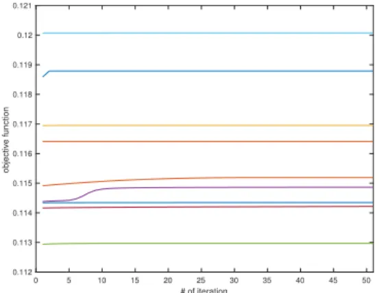
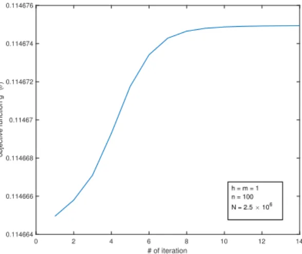
To solve (2.60), we first solve (2.61) to find a good initial point for (2.60). And then we apply the gradient assent method and at each iteration the objective function gn is estimated by the importance sampling scheme developed in Section 2.3.2. Some related technical details are discussed in Section 2.6.1 and Section 2.6.2. In Section 2.6.3, we set m= 1 and provide the settings for the minimization problem corresponds to the buffered probability.
2.6.1 Reformulation and solution of the limiting problem
Suppose that supθ∈Θinfβ≥0Lθ2(β)<Λ2. Then for eachθ∈Θ andβ ∈Rm, we have
ϕ1(β) +Lθ2(β)≥Λ2≥ inf β≥0L
θ
2(β) = inf β≥0(L
θ
2(β) +ϕ2(β)), (2.62)
by the definitions ofϕ1 and ϕ2 and the factLθ2(β)≥0. Then we have
g(θ) = inf β∈Rm
(ϕ(β) +Lθ2(β)) = inf
β∈Rm
(ϕ2(β) +Lθ2(β)) = inf
β∈Rm sup α∈Rm
h
ϕ2(β) +hα, βi −logEehα,G(X1,θ)i
i
.
(2.63)
For eachθ∈Θ define a function Φθ :Rm×Rm →Ras
Φθ(α, β) =ϕ2(β) +hα, βi −logEehα,G(X1,θ)i. (2.64)
differentiable, a saddlepoint of Φθ can be found by solving the following equations:
Oϕ2(β) +α = 0
β−OαlogEehα,G(X1,θ)i= 0.
So (2.61) can be written as
max θ∈Θ,α∈Rm,β∈
Rm
ϕ2(β) +hα, βi −logEehα,G(X1,θ)i
s.t. E[ehα,G(X1,θ)i]β = E[G(X
1, θ)ehα,G(X1,θ)i], 2Λ min(β,0) +α = 0.
(2.65)
The feasible set of the above optimization problem is not convex. However, a good feature of this problem is that the expectation in the objective function can be estimated by Monte Carlo simulation directly without importance schemes. In the numerical examples, we replace the expected values by an SAA and solve the problem with the interior point method to find a local minimum.
2.6.2 Implementing importance sampling in the gradient method
In the numerical examples, Xi is a normal random variable and the function G(x, θ) is piecewise linear in (x, θ). Then exp
−nϕ 1nPni=1G(Xi, θ) is Lipschitz continuous in θ with the same constant for allθ and almost surely differentiable with respect toθ. Applying [43, Theorem 7.49], the gradient ofgn atθ∈Θ is
Ogn(θ) = E
exp
−nϕ n1Pni=1G(Xi, θ) Oθϕ(1nPni=1G(Xi, θ))
Eexp−nϕ n1Pni=1G(Xi, θ)
, (2.66)
whereOθϕ(·) is the gradient ofϕ n1 Pni=1G(xi, θ)
with respect to θ.
Let ˆOgn(θl) be an SAA estimation of Ogn(θl). The update at thelth iteration is