EVALUATING THE INTERACTION OF GROWTH FACTORS IN THE UNIVARIATE LATENT CURVE MODEL
Stephanie T. Lane
A thesis submitted to the faculty of the University of North Carolina at Chapel Hill in partial fulfillment of the requirements for the degree of Master of Arts in the Department of
Psychology.
Chapel Hill 2014
iii ABSTRACT
Stephanie T. Lane: Evaluating the Interaction of Growth Factors in the Univariate Latent Curve Model
(Under the direction of Patrick Curran)
In the structural equation modeling framework, latent curve models have gained popularity for modeling change over time. Much work has focused on the use of covariates, whether time-invariant or time-varying, to predict the growth factors. Comparatively little work has focused on the use of growth factors as independent variables themselves. This project evaluated the performance of models where growth factors were used as main-effects predictors of a distal outcome; this main-effects-only model was expanded to include the interaction between the growth factors as a predictor. My results demonstrate the bias present when a main-effects-only model is fit to data where an interaction effect truly exists. These results provide motivation for researchers who employ growth factors as predictors of a distal outcome to test for an interaction effect in order to more clearly understand the role of
iv
TABLE OF CONTENTS
LIST OF TABLES ... vi
LIST OF FIGURES ... vii
CHAPTER 1: INTRODUCTION ... 2
The Latent Curve Model ... 6
Conditional Latent Curve Model... 9
Growth Factors as Predictors ... 9
Growth factors as Main Effects ... 10
Growth Factors as an Interaction Effect ... 11
Existing Methods for Estimating Latent Variable Interactions ... 13
Existing Approaches for Evaluating Interactions Among Latent Growth Factors ... 14
LMS ... 16
Goals... 18
CHAPTER 2: METHOD ... 19
Project... 19
Communalities ... 19
Effect Size ... 20
Sample Size ... 20
Repeated Measures ... 20
Parameters for Unconditional LCM ... 21
v
Hypotheses ... 25
Evaluation Criteria: Outcomes of Interest ... 25
CHAPTER 3: RESULTS ... 27
Model 1: Main Effects Only... 27
Summary of Model 1 Results ... 32
Model 2: Interaction ... 32
Summary of Model 2 Results ... 37
CHAPTER 4: DISCUSSION ... 38
Effect of Model Specification ... 39
Effects of Simulation Factors ... 39
Implications for Research... 41
Conclusion ... 44
APPENDIX A: SUPPLEMENTAL TABLES FOR MODEL 1, MAIN-EFFECTS-ONLY MODEL ... 60
APPENDIX B: SUPPLEMENTAL TABLES FOR MODEL 2, INTERACTION MODEL ... 73
vi
LIST OF TABLES
Table 1. Model 1: Main-Effects-Only, Factorial ANOVA for Bias in Parameter Estimates . 45
Table 2. Means and Bias for Model 1, Repeated Measures = 3 ... 46
Table 3. Means and Bias for Model 1, Repeated Measures = 6 ... 47
Table 4. RMSE for Model 1 Regression Parameters ... 48
Table 5. Empirical Power for Model 1 Regression Parameters ... 49
Table 6. Model 2: Interaction, Factorial ANOVA for Bias in Parameter Estimates. ... 50
Table 7. Means and Bias for Model 2, Repeated Measures = 3 ... 51
Table 8. Means and Bias for Model 2, Repeated Measures = 6 ... 52
Table 9. RMSE for Model 2 Regression Parameters ... 53
vii
LIST OF FIGURES
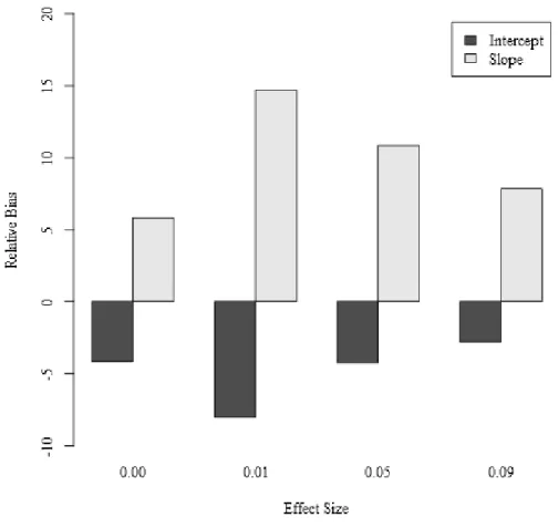
Figure 1. Growth Factors as Main Effects Predictors. ... 10 Figure 2. Growth Factors with Main Effects and Interaction Effect as Predictors. ... 12 Figure 3. Model 1, Main-Effects-Only, Relative Bias of and by Effect Size of . ... 55
2
CHAPTER 1: INTRODUCTION
In recent years, great emphasis in the behavioral sciences has been placed on reducing the incongruence between our motivating research questions and the methods with which we analyze our data. This effort has been particularly evident in the development of novel analytic strategies to address questions regarding the development of a construct over time. Thus, the last few decades have witnessed a shift away from cross-sectional data in favor of studies that bring longitudinal data to bear on our research questions regarding change over time. The shift toward longitudinal data collection has resulted in a corresponding surge of methods to evaluate change over time. Examples of these methods include the autoregressive cross-lagged model, random and fixed effects panel data models, the repeated measures multivariate analysis of variance (MANOVA) and the latent curve model (LCM) (Bollen & Curran, 2006).
3
the autoregressive model, we instead use our observed repeated measures as indicators of an underlying latent trajectory thought to give rise to the repeated measures over time.
Because of the emphasis on identifying and estimating an underlying trajectory, the latent curve model represents a closer match to the conceptualization of how growth unfolds over time in many domains. The structural equation modeling approach to the latent curve model allows researchers to draw on the many strengths of SEM; these strengths include readily available indices of fit, the ability to handle missing data, and the ability to
incorporate different forms of growth. To this effect, the latent curve model has become a standard approach to analyzing longitudinal data within behavioral sciences, from
applications examining the development of antisocial behavior over time (Curran, Bauer, & Willoughby, 2004) to applications examining alcohol use over time in adolescent females (Hipwell, Stepp, Chung, Durand, & Keenan, 2012).
An important strength of the latent curve model is its ability to approximate varying functional forms of change over time. Through the specification of fixed factor loadings relating the latent growth factors to the repeated measures observations, these trajectories can take the form of linear, quadratic, cubic, or other polynomial growth, as well as exponential, piece-wise, or freed-form growth (Bollen & Curran, 2006). Once the optimal factors
representing growth have been identified, they can then be predicted. This possibility is another strength of the latent curve model – its ability to incorporate exogenous predictors of level and change over time.
4
factors can be regressed onto time-invariant covariates in order to evaluate between-person predictors of level and growth. This flexibility also extends to a covariate assessed at multiple measurement occasions, which can be introduced as a predictor in the form a time-varying covariate. In such an example, the TVCs are regressed onto the repeated measures and the growth factors are interpreted net the effect of the TVCs (Bollen & Curran, 2006). Taken together, these aspects of the growth model allow us to make inferences about inter-individual differences in intra-inter-individual change over time.
To date, much work has focused on using exogenous covariates as predictors to explain variance in growth factors. However, little work has focused on the consequences of growth, or the potential to use the growth factors themselves as independent variables. As previously explicated, the growth factors thought to give rise to the repeated measures over time are often treated as dependent variables, with exogenous covariates frequently
introduced to the model in order to explain individual variability in the growth factors. Little work has focused on these growth factors as predictors of a distal outcome, yet the structural equation modeling approach to latent curve modeling allows us the flexibility to directly use growth factors as predictors. Thus, at this point in time, the issues involved in estimating, testing, and evaluating random growth factors as predictors in SEM are currently not well understood.
5
Schmiege, & Magnan, 2012; Hipwell et al., 2012), the predictive ability of the interaction effect between intercept and linear slope factors underlying a single construct has not been examined. An interaction effect among growth factors would suggest that the influence of the growth factors on an outcome is more than simply the additive effect of the two factors taken together. At this point, it is unclear whether the interaction effect between growth factors represents a further clarification of the conditional relations of the growth factors, or whether it is critical in the prediction of a distal outcome. In considering these issues, it is helpful to turn to a discussion of existing applications of growth factors as predictors.
A limited number of examples of growth factors as main effect predictors have been found in substantive areas of psychological research. In some instances, the growth factors for one variable are used to explicitly predict the growth factors for another variable; these variables are often measured concurrently (e.g., Bryan, Schmiege, & Magnan, 2012). Other instances of growth used as a predictor have arisen in the context of multilevel modeling where researchers are interested in using empirical Bayes estimates for intercept and slope to predict a distal outcome (e.g., Rowe, Raudenbush, & Goldin-Meadow, 2012).
6
intercept and slope factor were then used as predictors of later risky sex after age 16.
Researchers then expanded the model to conceptualize growth factors as mediators between time-invariant covariates (e.g., race, poverty status, pubertal status) and risky sex at a later age.
Taken together, these applied examples demonstrate an eagerness to expand the use of growth factors to be used as predictors. However, there is a need to first expand our understanding of the capacity of growth factors to serve as predictors. In order to continue the discussion of the latent curve model, I now turn to an analytic presentation of the latent curve model.
The Latent Curve Model
These models arise from the structural equation modeling (SEM) framework, where individual observations are fallible indicators of an individual’s true trajectory, defined by latent growth factors; commonly, these factors represent an intercept factor and a linear slope factor.
From the SEM framework, the factor analytic model relates the observed variables y
to the underlying latent construct η such that
(1)
(
) (
) (
) ( ) (
)
Where is a T × 1 vector of item intercepts, is a T × 1 vector of repeated measures, is a T × k matrix of factor loadings, and is a T × 1 vector of time-specific residuals. Because we
7
(2)
This simplifies the measurement model to:
(3)
The latent variable equation is
(4)
where is a k × 1 vector of factor means and is a k × 1 residual vector individual deviations from these means, and ( ) represents the covariance structure among the
latent factors.
The model implied variance of the reduced form is
(5)
where is the model implied covariance matrix of the ’s and represents the covariance structure of the disturbances for the T repeated measures of such that
( )
(6)
(
)
(7)
The expected value for the reduced form trajectory is
( ) (8)
8
For an equally spaced set of T = 4 repeated assessments and a linear trajectory, the 4 × 2 factor loading matrix is
(
)
(9)
With a 4 x 4 diagonal residual matrix
( )
(10)
And a symmetric covariance matrix among the random intercepts and linear slopes
(
)
(11)
The factor loadings relating the observed repeated measures to the slope factors are a combination of fixed and possibly free loadings that best capture the functional form of the growth trajectory. The initial approach is to fix the factor loadings to 0, 1, 2, 3, …T-1 to represent straight-line growth. The estimated mean of the intercept factor ( ) represents the
initial status of the trajectory averaged across all individuals; similarly, the estimated variance of the intercept factor ( ) represents the individual variability in starting point across all individuals. The estimated mean of the slope factor ( ) quantifies the slope averaged across all individuals, and the estimated variance of the slope ( ) represents
individual variability in rates of change over time. Finally, the covariance between the intercept and slope factors is denoted .
9
equivalent. Under the assumption of multivariate normality, the casewise likelihood of the observed data is obtained by maximizing the following function:
| | ( ) ( )
(12)
where is the vector of complete data for case i, and are matrices containing the
parameter estimates of the mean vector and covariance matrix, respectively, for variables complete for case , and is a constant that depends on the number of complete data points for case (Arbuckle, 1996; Enders & Bandalos, 2001). The discrepancy function is then
obtained by accumulating across the series and maximized as follows:
( ) ∑
(13)
Thus, all available data are utilized during parameter estimation. Conditional Latent Curve Model
The previous equations can be expanded to include a time-invariant covariate. Thus, we begin with our equation for the repeated measures, , in matrix notation
(14)
And expand the level 2 model to include covariates where
(15)
where is a k × 1 vector of factor means, is a k × p matrix of regressions of the factors on the TICs, is a p × 1 vector of TICs, and is a k × 1 residual vector individual deviations
from these means.
Growth Factors as Predictors
10
(16)
where is the outcome of interest, is the intercept for the outcome, and is a matrix of regression weights of the exogenous latent growth factor predictors, , of the distal outcome.
Growth factors as Main Effects
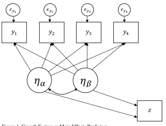
Before considering the estimation of an interaction effect among growth factors and its potential utility in predicting an outcome, we must first consider the meaning and the ability of growth factors when used as main effects predictors (see Figure 1).
Because of the estimated covariance(s) among growth factors, any main effect of one growth factor on a distal outcome would be interpreted as being above and beyond the effect(s) of any of the other growth factors. Just as in the conceptualization of main effects in a multiple regression, the regression coefficient of the distal outcome on one growth factor (e.g., the slope) is assumed to be equal across all levels of the other growth factor (e.g., the
𝑧
𝜂
𝛼
𝜖𝑦1
𝜖𝑦2 𝜖𝑦3 𝜖𝑦4
𝑦
𝑦
𝑦
𝑦
𝜂
𝛽
11
intercept). As a specific example, if a linear slope factor were to be used for prediction, its effect on an outcome would be interpreted in isolation. Therefore, the effect of the linear slope would be above and beyond the effect of the starting level or any form of polynomial growth over time. In other words, the effect of the linear slope on the outcome would be constant across all values of starting point, or intercept.
However, given the relationship between an individual’s starting point and change over time, it is difficult to conceptualize the predictive ability of linear change over time without any regard for an individual’s level, or starting point. In envisioning such an analysis, the linear slope for two individuals who shared a similar rate of change over time but had radically different starting points would be treated as the same. This fact is
immediately clear in the analyses, but its meaning is not; one could foresee a situation in which this would be less than desirable. With drug use as a specific example, an increase of X amount in drug use for an individual who had a high starting level would seem
qualitatively different than an increase of X amount in drug use for an individual who had a low starting level. This simple example highlights a broader need for the possibility of investigating an interactive effect between growth factors that could be then used as a predictor in conjunction with main effects.
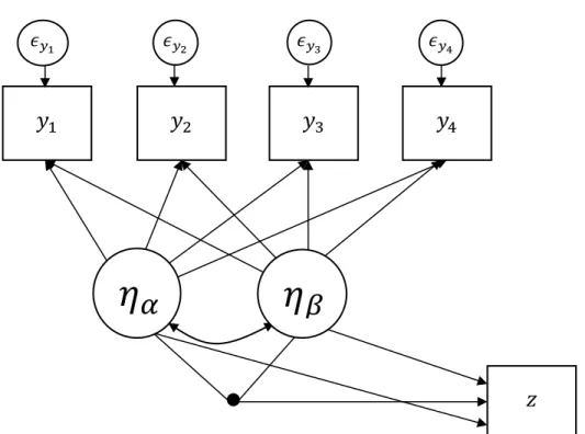
Growth Factors as an Interaction Effect
As previously mentioned, it may be possible that growth factors underlying a
12
levels of the other growth factor, there would be a different regression line of the outcome on a growth factor at each level of the other growth factor.
Conceptually, this could take the form of a buffering effect, where the level of one variable may buffer the impact of the other. Such a situation is commonly hypothesized in the context of multiple regression, with independent variables such as stress and social support (Aiken & West, 1991). Extending the idea of a buffering effect to the context of growth factors, it may be the case that starting level could buffer the influence of growth over time on an outcome for individuals who had lower starting levels on a construct. Put
differently, there could theoretically be a certain threshold of starting point at which the slope becomes more meaningful as a predictor.
𝑧
𝜂
𝛼
𝜖𝑦1
𝜖𝑦2 𝜖𝑦3 𝜖𝑦4
𝑦
𝑦
𝑦
𝑦
𝜂
𝛽
13
Alternatively, it may be the case that the interaction effect could be synergistic in nature, where individuals who both started a high level and grew more substantially over time could have a higher predicted outcome, above what would have been predicted by the intercept and slope factors independently. In considering the previously cited study with risky sex as an outcome (Hipwell et al., 2012), it could be the case that individuals with both high levels of drug use and high increases of drug use over time could have a higher
endorsement of risky sex than would have been suggested by the additive effect of the growth factors in isolation.
These brief examples highlight the need to investigate the interaction among growth factors more thoroughly, both conceptually and analytically. In order to consider the analytic issues that arise when considering an interaction effect among latent growth factors, I now turn to a discussion of previous techniques that have been developed for estimating
interactions among latent variables. I then extend this discussion to the current approaches for estimating interactions among latent growth factors.
Existing Methods for Estimating Latent Variable Interactions
14
intercept term. Due to the complicated nature of the constraints and phantom variables in specifying the model, these approaches were followed by a variety of two-step approaches (Bollen, 1995, 1996; Moosbrugger, Frank, & Schermelleh-Engel, 1991; Ping, 1996a, 1996b).
Finally, Klein and Moosbrugger introduced the latent moderated structural equations (LMS) approach, which explicitly takes into account the nonnormality present in latent interaction effects. Specifically, LMS represents the joint distribution of indicator variables as a finite mixture of normal distributions. Subsequently, Klein and Muthen (2007)
introduced a Quasi-Maximum Likelihood estimation procedure (Quasi-ML), which has less rigid distributional assumptions than LMS, and has been shown to be less computationally burdensome with more complicated models. Though LMS and QML largely overlap in the types of models that can be addressed by either approach, LMS is currently the standard for latent variable interactions, not only due to its availability in commercial software, but also due to its ability to build more complicated SEM models where there are multiple latent endogenous variables (Kelava et al., 2011). Therefore, for this project I will focus on LMS for the estimation of interactions among latent growth factors.
15
each model. The first two loadings for these shape factors were 0 and 1, followed by freed loadings to capture possible nonlinearity in the trajectories. The interaction between these shape growth factors was then captured by a factor defined by product indicators of the repeated measures for each construct. This factor defined by product indicators was then used to predict the slope growth factor of a distal outcome. Though a novel approach, it is unclear what the estimates from this model signify substantively. Additionally, this approach cannot readily be applied to the univariate case of evaluating an intercept-slope interaction in a single construct given that it relies on cross-products.
Another approach to modeling latent variable interactions, termed the latent variable score approach, was discussed by Schumacker (2002) after latent variable scores were developed by Joreskog (2000) in LISREL that satisfied the same relationships as latent variables themselves. Importantly, this latent variable score approach bypasses the usage of product indicators. Instead, latent variable scores, or factor scores, are directly created for each growth factor and then multiplied together. This product would then be used to test the interaction of the growth factors in the presence of the main effect of each growth factor. Though this approach has not yet been directly applied to growth models, the lack of
16 LMS
The latent moderated structural equations (LMS) approach was developed by Klein and Moosbrugger (2000) to provide a maximum likelihood estimation of model parameters for an interaction effect between latent variables. The LMS approach is built on two main premises. The first is that nonlinear effects, such as interaction effects, become linear when conditioned on the proper variable. Second, a multivariate distribution of indicator variables can be approximated by a weighted combination, or mixture, of normal distributions. Unlike other approaches, no manifest indicators are needed to estimate nonlinear effects. Instead, LMS estimates nonlinear effects by representing the nonnormal distribution of the joint indicator vector as a finite mixture of normal distributions (Moosbrugger, Schermelleh-Engel, Kelava, & Klein, 2008). LMS then applies Cholesky decomposition to the positive definite covariance matrix (m × m) of the latent exogenous variables ( ).
In the case of two latent exogenous variables, the Cholesky decomposition can be formally expressed as:
( )( ) (17) where is an ( ) identity matrix. The variables are then decomposed into mutually independent random variables . This matrix, , is then replaced by the vector product of a vector ( ) with itself. Each variable from the vector is standardized, normally distributed ( ), and orthogonal to the variables remaining. The
decomposition of replaces the correlated variables by an matrix and by the vector of independent variables. This vector ( ) is then partitioned into vectors and
17
( ) (18)
where ( ) and ( ) The first elements in are the variables that correspond to the variables involved in nonlinear terms. This procedure creates
orthogonal components that allow partitioning of the distribution of the variables into linear and nonlinear parts (Kelava et al., 2011). The vector is used as the conditioning variable upon which the joint distribution of and is conditionally multivariate.
Finally, a mixture distribution is used to represent the multivariate distribution of the and variables where is used to determine means, variances, and covariances of the set
of normal distributions used in the mixture. These normal distributions are then weighted and summed to represent the multivariate distribution of the observed variables.
Hermite-Gaussian quadrature is used to approximate the mixture distribution where the weights used by this process provide the best approximation of the multivariate surface. LMS utilizes the mixture distribution and adapts the Expectation-maximization (EM) algorithm to provide parameter estimates (Dempster, Laird, & Rubin, 1977). LMS also allows for the estimation of standard errors by calculating the Fisher information matrix (Klein & Moosbrugger, 2000). Wald z tests can then be used to compare each parameter estimate and its corresponding standard error.
18 Goals
The goal of my project is to describe the incorporation and meaning of an interaction among latent growth factors and to analytically articulate the latent curve model with an interaction effect. In order to do this, I will first describe the treatment of latent growth factors as predictors of a distal outcome. I aim to discuss the conditions under which growth factors are adequate in isolation as predictors and to evaluate the finite sampling behaviors of a growth factors as main effects model.
19
CHAPTER 2: METHOD Project
In order to assess the meaning and utility of growth factors as predictors, I conducted a series of computer simulations. I simulated longitudinal data consistent with a univariate linear latent curve model; this simulation included a distal outcome that was a function of the latent factors. All data generation was conducted in R; data analysis was conducted in Mplus; outcomes of interest were calculated in R.
In order to address my research aims, I conducted a simulation under varying conditions commonly encountered in behavioral research to evaluate the finite sampling behavior of these models. I first evaluated the finite sampling behavior of a model (Model 1) where the interaction effect was not modeled. I then demonstrated the anticipated bias that would be present in a main-effects-only growth model in the presence of an unmodeled interaction effect. I now turn to a discussion of the simulation factors that were varied for the study.
Communalities
20
was anticipated that higher communalities would result in better detection of the interaction effect.
Effect Size
The effect size of the interaction between the growth factors on the distal outcome was also varied in this study. Data were generated such that there were four conditions of effect size for the interaction term, where the interaction uniquely explained 0, 1, 5, and 9 percent of the variance in the distal outcome, corresponding to cutoff values for zero, small, small-to-moderate, and moderate effect size (Cohen, 1988).
Sample Size
The sample size was varied at N = 200 and N = 400. I selected the upper bound of N = 400 because it is a relatively large but reasonable sample size for longitudinal research in the social and behavioral sciences; importantly, this sample size has been used successfully in simulation studies involving LMS (Kelava et al., 2011). Similarly, I chose a sample size of N = 200 because it has been suggested that LMS may perform with samples of at least this size if the model is relatively simple, as in the case of a single interaction effect (Kelava et al., 2011). Though there are no explicit cutoffs for sample size in the latent curve model, sample sizes exceeding N = 100 are preferred (Curran, Obeidat, & Losardo, 2010). Repeated Measures
Finally, there is no reliable rule of thumb that dictates the optimal number of repeated measures, but it has been recommended that linear models have at least four to five
21
encountered in practice: three and six repeated measures. These repeated measures were equally spaced in time. The repeated measures were generated to be multivariate normal. This is not always a tenable condition in practice; however, it was maintained for the current study so that other conditions could be investigated.
Therefore, there were a total of ninety-six conditions (models × 2, communalities × 3, effect size × 4, sample size × 2, number of repeated measures × 2), and these conditions were assessed over R = 1000 replications. While important, missing data was not investigated in the course of this study given the desire to evaluate the performance of these models under more optimal conditions. Additionally, under missing at random (MAR), theory would not predict that missing data would substantially affect results in a manner different from expectation.
Parameters for Unconditional LCM
The parameters used in the simulation were adapted from mean and variance estimates from a subset of data pertaining to alcohol use in adolescence (Curran, Stice, & Chassin, 1997). The parameters for the unconditional LCM correspond to an intercept with a mean of and a slope of . The variance of the intercept is and the
variance of the slope is . The covariance between the intercept and slope is
, which corresponds to a correlation of .24. The repeated measures are equally
spaced and represent linear growth over time. The residual variances at each time point are varied to correspond to communalities of .4, .6, and .8 for the repeated measures, as
demonstrated below.
Repeated measures = 3
22 [
]
[ ]
Communality = .4
(
)
Communality = .6
(
)
Communality = .8
(
)
Repeated measures = 6; all as above except:
[ ]
Communality = .4
(
)
23
(
)
Communality = .8
(
)
For the generation of the distal outcome, the beta weights for the effect of the intercept and slope on the distal outcome correspond to standardized coefficients of 0.2. These standardized values were calculated using the formulas below (Muthén, 2012):
√ ( )
√ ( ) (19)
√ ( ) √ ( )
(20)
where each unstandardized coefficient is divided by the standard deviation of the distal outcome and multiplied by the standard deviation of the respective latent growth factor. Finally, the standardized estimate for can be obtained by the formula:
√ ( )√ ( )
√ ( ) (21)
24
respectively; these squared semi-partials reflect the percentage of variance in the distal outcome uniquely explained by the interaction of the growth factors. The unstandardized coefficients for the interaction across the four effect size conditions correspond to
standardized coefficients of 0, .10, .22, and .29. The variance of the distal outcome was set to ( ) , and the residual variance diminishes across the three conditions as the unique
variance explained by the interaction increases. Generating Distal Outcome
Interaction
[
( )( )]
( )
( )
Interaction
( )
Interaction
( )
Interaction
25 ( )
Hypotheses
In the main-effects only model (Model 1), I anticipated that the main effects would be increasingly biased as the effect size for the unmodeled interaction effect increased.
Additionally, given the anticipated positive bias of the main effects, I expected there to be an inflated empirical rejection rate when detecting these main effects across increasingly higher values of effect size for the unmodeled interaction.
In the interaction model (Model 2), I expected that there would be greater power to detect the interaction effect when its squared semi-partial was higher. Specifically, the proportion of false negatives will decrease. Additionally, I anticipated that there would be greater power to detect the interaction effect when sample size, communalities, and number of repeated measures were higher. I did not expect substantial bias otherwise, as I was fitting the data-generating model to its corresponding data.
Evaluation Criteria: Outcomes of Interest
26
Raw bias is defined as the true population value ( ) subtracted from the average sample estimate ( ̂)
̂ (22)
Relative bias was calculated as
̂
(23)
RMSE was computed as
√∑( ̂) (24)
Empirical power was calculated as the proportion of times that the null hypothesis was rejected when the null hypothesis was false. The raw bias across conditions of the simulation was analyzed using a four-factor analysis of variance (ANOVA). This 4×3×2×2 ANOVA detected any significant main or interaction effects, and I followed this analysis with specific contrasts. I then computed effect size using partial , calculated as
(25)
where I consider effects above with a partial value above the cutoff of I then
CHAPTER 3: RESULTS
I will begin by presenting Model 1, the main-effects-only model. I will then continue to Model 2, the properly specified model where the interaction effect is included.1 I will begin by presenting results where the effect size for the interaction has been set to zero, averaging across all other simulation factors. These results will demonstrate the Type I error rates for estimating the interaction effect using LMS. After the presentation of Type I error, I will proceed to examine partial values from ANOVA meta-models above the cutoff ; I then present relative bias for parameters with a non-zero population generating value.
Descriptively, I follow this with relevant RMSE values. Model 1: Main Effects Only
Results were discarded if the estimation failed to terminate normally. This would result in Mplus failing to print standard errors. A total of 5856 replications out of 48000 were discarded, representing 12.20% of replications for this condition. Results were also excluded from analysis if the standard errors for parameter estimates exceeded 4 standard deviations above or below the mean of the standard error for that condition. This was done to catch unrealistic standard errors that were missed in the previous step. The conditions most affected were those where repeated measures = 3 and the effect size of the (unmodeled) interaction was = .09. In contrast, regardless of effect size, the conditions with six
repeated measures experienced almost no losses due to convergence issues.
1
28
A total of 102 replications were discarded in this screening, representing 0.22% of all runs. This left 42144 cases, or 87.80% of the original replications. The analyses below make use of this restricted subset.
The ANOVA meta-model results examining bias in the parameter estimates are presented in Table 1. In this table, values in parentheses represent the partial values for each effect, and partial values exceeding .06 are bolded for ease of presentation. The
mean, raw bias, and relative bias for the regression parameters are presented in Tables 2-3, and the RMSE values for and are presented in Table 4. Finally, power for and
across the various conditions is presented in Table 5.
The standard errors of the parameter estimates were also examined in this study. Given the aim to discuss results for the most relevant parameters, information regarding standard errors is presented in Appendix A for the interested reader. Appendix A contains information for the ANOVA meta-model results examining bias in the standard errors of the full set of parameter estimates. The mean, raw, bias, relative bias, and RMSE for the non-regression parameters, , , , , and are also presented in Appendix A.
Finally, for the full set of parameters, the standard deviation of the parameter estimate, average standard error, raw bias, relative bias, and corresponding RMSE are presented in Appendix A.
29
Across conditions, the relative bias for remains under 10% in the properly specified model. With the exception of one condition, the relative bias for similarly
remains under 10%. Where communalities, sample size, and repeated measures are low, the relative bias for is 13.79%. Thus, even in the least optimal of conditions for fitting a
main-effects only model in practice, the relative bias remains relatively modest. These results serve as a verification of proper data generation, as we are observing negligible bias where the data-generating model is being fit to its corresponding data.
Part 2: Misspecified Model. The following results detail findings where a main-effects-only model has been fit to data with a non-zero effect size for the effect of the
interaction on the distal outcome. Multiple effects were present in examining the effect of the simulation factors on the bias of parameters of interest. The most important of these effects pertained to the regression parameters ( , ). Other effects were present for the means of the latent factors ( and ), as well as the variance of the slope factor ( ). Here, I
discuss in depth the outcomes pertaining to the regression parameters, or the main effects of the latent factors on the distal outcome. I then briefly summarize the factors influencing bias in the mean and variance of the latent factors. I follow this with a discussion of power and a summary of Model 1 results.
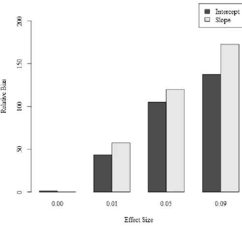
Intercept effect on outcome, . The effect size of the (unmodeled) interaction effect had the most demonstrable effect on the bias of , the main effect of the intercept on the outcome, where partial . A nontrivial portion of this effect is due to the fact that the properly specified model ( = .00) is one level of the effect size factor. Specifically, the
30
107.14%, and 139.88% (see Figure 3). Additionally, the spread of errors of prediction
increased with increasing effect size. For example, for repeated measures = 3, communality = .6, and n = 200, the RMSEs for were 0.42, 0.46, 0.74, and 0.86 across increasing effect
size. This pattern indicates that the discrepancy between the observed and predicted values increases alongside the amount of bias in the parameter estimate caused by the effect size of the unmodeled interaction.
Slope effect on outcome, .A similar pattern was observed for the bias present in the effect of the slope on the outcome, where the size of the interaction effect had the most demonstrable effect on the bias of the main effect of the slope on the outcome, partial
. Again, the relative bias in the slope parameter increased as the size of the
unmodeled interaction effect increased, with relative bias values of 0.40%, 58.17%, 120.70%, and 173.83% (see Figure 3), corresponding to the respective conditions. As with , the RMSE values increased with increasing effect size for ; for example, for repeated measures = 6, communality = .6, and n = 400, the RMSEs for were 0.26, 0.60, 1.02, and 1.66 across the respective conditions. These values represent contribution of
the bias and the sampling variability, so that estimates are increasingly biased and variable as the size of the unmodeled interaction increases.
Power for and in Model 1. Because of the misspecification, the values to which I am referring as power could be better thought of as power augmented by an inflated empirical rejection rate. As anticipated, the proportion of significant estimates for and
31
respectively. For and , the power increased as the effect size of the unmodeled
interaction effect increased. For example, with communalities = .4, n = 400, and three repeated measures, the power to detect was 0.32, 0.65, 0.74, and 0.80 across increasingly higher values. Thus, for the regression of the distal outcome on the latent intercept and
slope, power increased as the parameter estimates became more positively biased due to the increasing magnitude of the unmodeled (positive) interaction effect.
Summary of other parameters.
Across the parameters pertaining to the mean and variance of the latent factors, multiple main and interaction effects with partial values exceeding .06 were present. For
ease of presentation and to retain scope, only main effects will be presented briefly. For both the mean of the intercept factor and the variance of the slope factor, the relative bias in the parameter estimate decreased for repeated measures = 6 compared to repeated measures = 3, averaging over all other simulation factors. Note that this comparison does not occlude conditional effects, but instead focuses on the main effect in isolation. For example, the RMSE value for is .06 at repeated measures = 3, when n = 200, = 0, and
communalities = .8 and is .03 when repeated measures = 6, holding other factors constant. Similarly, when n = 200, communalities =.6, = .09, we see that the relative bias of
goes from 16.04% to 0.68% when moving from 3 to 6 repeated measures, averaging over all other conditions.
32
0.04, 0.04, and 0.03 across increasing effect size when n = 200, communality = .8, and repeated measures = 3. Taken together, the effects pertaining to the mean and variance of the latent factors are modest in size and do not behave in a manner different from expectation. Summary of Model 1 Results
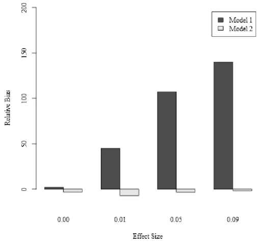
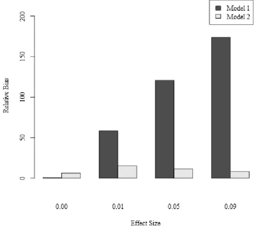
Overall, these results demonstrate the substantial bias present in a model where an unmodeled interaction effect exists. The most prominent of these effects pertain to the bias present in the main effects of the growth factors on the distal outcome. With increasing effect size of the unmodeled interaction effect, the main effects become increasingly biased. For a side-by-side demonstration of this, see Figure 3. Other simulation factors that do not affect the regression parameters, but instead affect the recovery of the parameters pertaining to the mean and variance of the growth factors, result in small amounts of bias. Finally, the
simulation factors affect power in a pattern consistent with expectation. Model 2: Interaction
For the models, results were discarded if the estimation failed to terminate normally due to nonconvergence. This would result in Mplus failing to print standard errors.
Additionally, results were discarded if a warning message was presented that indicated that the "model estimation has reached a saddle point or a point where the observed and the expected information matrices do not match." This warning appears when the optimization algorithm reaches a saddle point; it then produces standard errors that are calculated using the MLF estimator, or maximum likelihood with first-order derivative standard errors
33
standard errors were of interest in this project, these results were discarded. A total of 1546 replications were discarded due to these two factors, representing 3.22% of all runs for the interaction-effect model. The number of complete replications was affected most in conditions where n = 200, repeated measures = 3, and communality = .4.
Using the same outlier screening as before, an additional 102 cases were removed, representing 0.22% of all cases. This left 46352 runs, or 96.57% of all replications. The analyses below make use of this restricted subset.
The ANOVA meta-model results examining bias in the parameter estimates are presented in Table 6 for multiple parameters of interest: , , , , , , , , and
. In this table, values in parentheses represent the partial values for each effect, and
partial values exceeding .06 are bolded for ease of presentation. The mean, raw bias, and
relative bias for the regression parameters are presented in Tables 7-8, and RMSE values for the regression parameters are presented in Table 9. Finally, power for , , and is
presented in Table 10.
The ANOVA meta-model results examining bias in the standard errors of the parameter estimates are presented in Appendix B for the aforementioned parameters of interest: , , , , , , , , and . The mean, raw bias, relative bias, and
RMSE for , , , , , and are presented in Appendix B. For the full set of
parameters, the standard deviation of the parameter estimate, average standard error, raw bias, relative bias, and RMSE are presented in Appendix B.
34
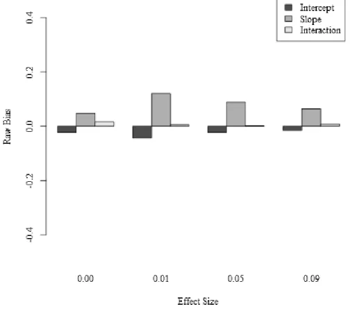
repeated measures = 6, communality = .8, and sample size = 400. These selections represent more optimal conditions encountered in practice. Collapsing across the non-zero effect size values ( .01, .05, and .09), the average relative bias for , , and is
0.12%, -0.16%, and -0.08%, respectively. This demonstration illustrates the ability of LMS to recover a non-zero interaction and serves as verification that the data were properly generated.
Type I error. Averaging over all other simulation factors (repeated measures, communality, and sample size), I examined the proportion of cases that resulted in a significant estimate for the regression of the distal outcome on the interaction between the latent factors in the condition when Model 1 was applied to the data. The Type I
error rate was .036, indicating that 3.6% of interaction effects were significant in the
condition where they were set to zero by design. Looking across conditions, the Type I error rate ranged from .027 to .045, where the highest rates were observed at lower repeated
measures and lower sample size. No individual condition exceeded Thus, the Type I error rates across conditions where were all below the standard cutoff of ,
indicating that the null hypothesis is not rejected more than the nominal rate.
Summary of main and interactive effects on outcome ( , , ): For the
regression of the distal outcome on the growth factors and the interaction between the growth factors, there were no substantial effects according to the partial values. That is, according
to the ANOVA meta-model, the properly specified model recovered the effects without any simulation factor contributing to bias in the parameter estimates above the specified partial
35
However, differences can still be seen by examining individual conditions. For
example, with repeated measures = 3, , n = 200, and communality = .4, the relative bias in is -41.58%, the relative bias in is 46.98%, and the relative bias in is 39.65%. In contrast, with all as above but communality = .8, the relative bias for is 3.36%, the relative bias for is 9.39%, and the relative bias for is -8.45%. This relative bias is
further reduced when considering the same parameters at n = 400, holding other conditions constant.
This pattern is also present in the RMSE values. For example, for , the RMSE
value is 0.75, 0.50, and 0.39 for communalities of 0.4, 0.6, and 0.8, respectively, at repeated measures = 6, , and n = 200. For the same conditions, increasing to n = 400, the
RMSEs further decrease to 0.42, 0.31, and 0.23, respectively. Importantly, these RMSE values also demonstrate the degree of spread in the estimates for the regression parameters, even in a properly specified model.
Summary of other parameters. For both the mean of the intercept factor and the mean of the slope factor, there was a main effect of repeated measures and effect size of the interaction. However, for the mean of the latent intercept, both the main effect of repeated measures (partial ) and effect size of the interaction (partial ) show
negligible relative bias, under 3%. Similarly, for the mean of the slope factor, the main effects showed negligible differences in relative bias across increasing effect size and across repeated measures, with relative bias <5%. Further investigating the main effect of repeated measures, the RMSE value for is .14 at repeated measures = 3, when n = 200, = 0,
36
variability in parameter estimates than was observed in the RMSE values for the regression parameters.
An interaction between sample size and effect size presented itself for ; however, though this effect (partial ) exceeded our cutoff, the relative bias across the levels of
these conditions hovers around 5%. Thus, even the most substantial of the effects did not produce troublesome bias. From the most substantial of the interaction effects for , we see that the amount of bias across values is lower as communalities increase. We again have
a small effect, as the relative bias remains under 10% across these conditions.
Power in Model 2. As anticipated, the proportion of significant estimates for , , and increase with a) higher sample size, b) higher communalities, and c) more repeated measures. For example, with six repeated measures, n = 400, and for the interaction, the power to detect was .36, .64, and .83 with communalities of .4, .6, and .8, respectively. For , the power increased as the proportion of variance in the distal outcome uniquely
explained by the interaction increased. For example, with communalities = .6, n = 200, and six repeated measures, the power to detect was 0.03, 0.36, 0.74, and 0.99 across
increasingly higher values. Demonstrating the impact of sample size and number of repeated measures, where .05, and communality = .4, the empirical power to detect
37 Summary of Model 2 Results
Taken together, though there are no main or interactive effects of simulation factors on the key regressions in Model 2: , , careful examination across conditions reveals cell-to-cell differences that behave as predicted. The effects that exceed the partial cutoff
38
CHAPTER 4: DISCUSSION
For this study, I employed a simulation study to evaluate my hypotheses regarding the inclusion of an interaction effect among growth factors as a predictor of a distal outcome. This is the first study to evaluate the estimation and inclusion of an interaction among growth factors in a univariate latent curve model and to rigorously test the finite sampling behavior of these models under conditions researchers may commonly encounter in practice. This study furthers current knowledge regarding the performance of LMS by extending previous simulation work (e.g., Kelava et al., 2011). Additionally, where prior research has focused on an intercept-covariate interaction within the latent curve model (Sun & Willson, 2009), this study focuses on the predictive utility of the interaction between the growth factors.
39 Effect of Model Specification
The proper specification of the model was shown to be crucial. I initially hypothesized that the main effects would be biased in the presence of an unmodeled interaction effect, and the results supported this prediction. Importantly, this bias should be interpreted as over-estimation. We observed that the properly specified model performed well and the misspecified model performed poorly; we would expect this outcome under proper data generation.
Effects of Simulation Factors
Before the discussion of each individual simulation factor, it is important to first note the variability in certain parameter estimates that likely affected why some partial values
exceeded the cutoff while others did not. For the parameters pertaining to the mean and variance of the latent factors, the distribution of bias within each cell did not fluctuate tremendously across simulation conditions. For example, in Model 2, the RMSE for was 0.14 for a sample size of 200 with three repeated measures, = 0 and communality = .4.
The RMSE value for the same conditions with communality = .8 was 0.06. At higher sample size and higher repeated measures, the discrepancy in RMSE values across levels of
communality is diminished. These values demonstrate that there is less variability in the parameter estimates as the simulation conditions become more optimal, but that even the least optimal of conditions do not produce troublesome RMSE for the parameter estimates pertaining to the mean and variance of the latent factors.
By contrast, there was much more fluctuation in parameter estimates for the
40
communality = .4). In contrast, the RMSE reduced drastically to 0.12 in what could be considered the most optimal of conditions ( .00, repeated measures = 6, sample size = 200, communality = .8). Given that the partial is calculated as a ratio of and
(see Equation 25), it is likely the case the large amount of within-cell
variability for the regression parameters overwhelmed the meaningful degree of between-group differences witnessed in the relative bias across conditions.
This variability at least in part explains why partial values for effects pertaining to
the mean and variance of the latent factors exceeded the cutoff, but upon further
investigation, produced differences in relative bias across conditions <10%. On the other hand, there were substantial differences in relative bias for the regression parameters across varying combinations of the levels of the simulation factors that did not meet the criteria for partial . With this consideration in mind, I now turn to a discussion of the effects of the
simulation factors.
Effect of Sample Size and Number of Repeated Measures. Regarding the effects of sample size and repeated measures, I hypothesized that there would be greater power to detect the interaction when the sample size and the number of repeated measures were
higher. This pattern was largely supported. Finally, though all Type I error rates stayed below the nominal .05 level, the highest of the Type I error rates that were observed occurred
in cells where the sample size and the number of repeated measures were small.
41
already small amount of relative bias in the regression parameters decreased slightly as communalities increased.
In Model 2, multiple effects involved the communality factor. Power for the
regression parameters was greater at higher communalities. Additionally, high communality served to protect from loss of power at a small number of repeated measures and a smaller sample size. For example, at a communality of .4, there was a substantial increase in power when sample size or number of repeated measures increased; this increase in power exceeded 30% for some cells. Conversely, at a communality of .8, there was a negligible increase in power (< 2%) across increased sample size and number of repeated measures.
Impact of Effect Size. My initial hypothesis was that the power to detect the interaction effect would increase as its unique contribution to the variance of the distal outcome increased. This conclusion was supported, where power ranged from .88 to <1 for the condition where the effect size for was .09, spanning over all other conditions.
That is, even in the least optimal of conditions in countered in practice (small number of repeated measures, low communality, and small sample size), there was sufficient power to detect an interaction corresponding to a moderate effect size.
Implications for Research
From this, several implications for applied and quantitative research arise. The first is that, when using growth factors as predictors of a distal outcome, the interaction effect should also be considered and tested for. My results demonstrate that, at best, testing for an interaction that truly exists will protect the researcher from potentially overinterpreting main effects that are positively biased due to an unmodeled positive interaction effect or,
42
negative interaction effect. If researchers test for an interaction and find that no interaction exists, I demonstrated that the main effects will not be biased by testing for this interaction. Thus, much like is done in the standard two-way ANOVA, testing for an interaction among growth factors when using growth factors as predictors should become standard practice. Much like in the standard multiple regression model, this interaction can be probed such that the strength of the influence of on z ( ) is moderated by This representation
matches the conceptualization of the slope as a focal predictor and the intercept as the moderator, where the effect of growth over time on a distal outcome depends on the individual’s initial starting point.
Importantly, these results represent a unique contribution beyond existing knowledge pertaining to testing interactions in multiple regression. The process of testing interactions in LCM introduces the unique challenges of 1) estimating an interaction among latent, not observed, variables, 2) having latent variables defined by the same repeated measures, and 3) retaining the mean structure of the growth factors.
Limitations and Future Directions
The present study is not without limitations. Given the possible number of factors that could have been varied in the study, several potentially interesting factors were not
considered for this project. Four factors that were not investigated that could have impacted the results in meaningful ways were the 1) normality of the repeated measures, 2) the
measurement scale of the repeated measures, 3) the sign of the regression parameters, and 4) the method of estimating the interaction between the latent variables.
non-43
normality of the repeated measures could have been varied to mimic observations that may be encountered more often in practice. However, I do not anticipate that the non-normality would have impacted the results differently than one might hypothesize. Indeed, LMS is known to be biased in the presence of nonnormality, as it only able to approximate the nonnormality due to the interaction; under this condition, QML may be the better choice of estimator (Kelava et al., 2011). Similarly, repeated measures in practice are frequently
composed of items that may be ordinal in nature, where a researcher has a five- or seven-item scale. Again, this was not examined to retain scope, and results would have likely not been present that went against expectations.
Additionally, the direction of the effects of the growth factors and the corresponding interaction on the distal outcome was not varied. That is, the main effects and interaction effect were all generated to be positive. In the results for the main-effects-only model, we observed that this unmodeled interaction effect positively biased the main effects, which in turn increased the rejection rate of the null hypothesis. A condition with positive main effects and a negative unmodeled interaction effect was not examined, nor was a condition with negative main effects and a positive interaction effect.
Finally, the method of estimating the interaction effect was not varied. The current study used LMS, but QML could have been evaluated as well as an alternative method of estimating the interaction between the latent factors. However, LMS and QML are known to perform similarly under several of the conditions that were varied in my study (Klein & Muthén, 2007); other simulation factors would better serve a study comparing the
44
potential use among substantive researchers aiming to include an interaction effect (e.g., McCarty et al., 2013). Future projects would do well to consider these additional factors for further study.
Conclusion
Taken together, this project presents numerous insights for further consideration. Among the most important points is that the main effects of interest will be biased in the presence of an unmodeled interaction effect, and that the magnitude of this bias will increase as the size of the unmodeled interaction effect increases. Depending on the sign and
magnitude of the main and interaction effects, this bias could take the form of a spurious finding or could result in a null finding where an effect truly exists.
45
Table 1.
Model 1: Main-Effects-Only, Factorial ANOVA for Bias in Parameter Estimates
Factor df
n 1 101.38(0) 191.18(0) 1.69(0) 224.44(0.01) 888.53(0.02) 646.59(0.02) 7.78(0) 3.51(0)
comm 2 73.82(0) 18.22(0) 109.08(0.01) 526.25(0.02) 744.98(0.03) 174.87(0.01) 583.92(0.03) 621.17(0.03)
sr 3 15416.69(0.52) 19795.26(0.59) 10261.22(0.42) 226.45(0.02) 643.97(0.04) 1038.75(0.07) 322.12(0.02) 308.46(0.02)
rm 1 228.72(0.01) 89.17(0) 176.09(0) 4517.22(0.1) 3485.91(0.08) 5778.89(0.12) 652.11(0.02) 2835.55(0.06)
n*comm 2 69.88(0) 22(0) 66.14(0) 190.26(0.01) 849.46(0.04) 226.01(0.01) 33.29(0) 67.87(0)
n*sr 3 19.69(0) 35.48(0) 61.53(0) 10.78(0) 3765.75(0.21) 293.36(0.02) 310.69(0.02) 130.06(0.01)
n*rm 1 200.75(0) 0.1(0) 194.26(0) 242.15(0.01) 1953.53(0.04) 1379.36(0.03) 751.75(0.02) 49.39(0)
comm*sr 6 24.33(0) 41.13(0.01) 49.13(0.01) 303.6(0.04) 1314.5(0.16) 469.71(0.06) 356.08(0.05) 93.32(0.01)
comm*rm 2 24.92(0) 76.91(0) 26(0) 1253.03(0.06) 948.07(0.04) 38.22(0) 31.25(0) 808.96(0.04)
sr*rm 3 50.33(0) 45.71(0) 123.05(0.01) 679.09(0.05) 575.82(0.04) 178.17(0.01) 100.18(0.01) 345.07(0.02)
n*comm*sr 6 18.79(0) 11.14(0) 12.8(0) 82.64(0.01) 183.99(0.03) 1088.28(0.13) 297.15(0.04) 53.32(0.01)
n*comm*rm 2 18.25(0) 1.69(0) 18.49(0) 377.95(0.02) 1121.4(0.05) 3.03(0) 99.31(0) 15.93(0)
n*sr*rm 3 126.55(0.01) 56.52(0) 473.95(0.03) 267.06(0.02) 1850.74(0.12) 1608.31(0.1) 327.22(0.02) 151.81(0.01)
comm*sr*rm 6 8.81(0) 26.25(0) 38.32(0.01) 130.93(0.02) 662.15(0.09) 550.04(0.07) 279.55(0.04) 250.33(0.03)
n*comm*sr*rm 6 10.12(0) 8.28(0) 29.32(0) 202.5(0.03) 1720.07(0.20) 1518.64(0.18) 127.09(0.02) 65.32(0.01)
Residuals 42096
46
Table 2.
Means and Bias for Model 1, Repeated Measures = 3
Effect Size = .00 Effect Size = .01 Effect Size = .05 Effect Size = .09
Parameter (pop. value)
M Raw Bias Rel.Bias M Raw Bias Rel.Bias M Raw Bias Rel.Bias M Raw Bias Rel.Bias
Communality = .4 N = 200
(0.54) 0.54 0 0.51 0.89 0.36 66.85 1.13 0.60 112.34 1.49 0.96 179.04
(0.82) 0.93 0.11 13.79 1.22 0.4 49.57 1.78 0.96 117.93 2.18 1.37 167.22
N = 400
(0.54) 0.53 0 -0.33 0.74 0.21 38.82 1.13 0.59 110.88 1.22 0.69 128.56
(0.82) 0.85 0.03 4 1.38 0.57 69.48 1.89 1.07 131.42 2.29 1.47 180.48
Communality = 0.6 N = 200
(0.54) 0.55 0.02 3.81 0.83 0.30 56.19 1.22 0.68 127.87 1.38 0.84 157.82
(0.82) 0.80 -0.02 -2.56 1.23 0.41 50.21 1.56 0.74 90.63 2.12 1.30 159.76
N = 400
(0.54) 0.55 0.01 2.51 0.75 0.21 40 1.20 0.66 124.27 1.35 0.81 152.41
(0.82) 0.81 -0.01 -1.35 1.27 0.45 55.29 1.79 0.97 118.71 2.05 1.23 151.17
Communality = 0.8 N = 200
(0.54) 0.56 0.03 5.13 0.82 0.29 54.33 1.12 0.58 109.18 1.39 0.86 160.36
(0.82) 0.80 -0.02 -1.86 1.26 0.44 54.41 1.69 0.88 107.35 2.24 1.42 173.91
N = 400
(0.54) 0.53 -0.01 -1.24 0.75 0.22 40.82 1.04 0.51 95.11 1.26 0.72 135.03
47
Table 3.
Means and Bias for Model 1, Repeated Measures = 6
Effect Size = .00 Effect Size = .01 Effect Size = .05 Effect Size = .09
Parameter (pop. value)
M Raw Bias Rel.Bias M Raw Bias Rel.Bias M Raw Bias Rel.Bias M Raw Bias Rel.Bias
Communality = .4 N = 200
(0.54) 0.58 0.04 8.35 0.81 0.28 52.28 1.19 0.65 122.11 1.26 0.73 136.17
(0.82) 0.77 -0.04 -5.22 1.22 0.4 49.07 1.83 1.02 124.63 2.17 1.35 165.81
N = 400
(0.54) 0.55 0.01 2.77 0.73 0.2 37.4 1.08 0.55 102.12 1.28 0.74 138.95
(0.82) 0.81 0 -0.34 1.28 0.46 56.39 1.89 1.07 131.03 2.37 1.55 190.2
Communality = .6 N = 200
(0.54) 0.55 0.02 2.88 0.7 0.17 31.87 1.14 0.6 113.13 1.2 0.67 124.53
(0.82) 0.82 0 0.58 1.32 0.5 61.36 1.7 0.89 108.41 2.27 1.45 177.48
N = 400
(0.54) 0.54 0.01 1.23 0.77 0.24 44.35 1.04 0.51 94.9 1.32 0.79 147.71
(0.82) 0.82 0 -0.13 1.36 0.55 67 1.81 1 121.96 2.48 1.66 203.16
Communality = .8 N = 200
(0.54) 0.53 0 -0.13 0.74 0.2 37.77 1.04 0.5 93.95 1.14 0.61 114.01
(0.82) 0.82 0 0.49 1.33 0.51 62.37 1.94 1.12 137.31 2.07 1.25 152.99
N = 400
(0.54) 0.53 0 -0.55 0.78 0.25 46.75 1.04 0.51 94.96 1.3 0.76 142.67
48
Table 4.
RMSE for Model 1 Regression Parameters
Communality = .4 Communality = .6 Communality = .8
Effect Size 0.00 0.01 0.05 0.09 0.00 0.01 0.05 0.09 0.00 0.01 0.05 0.09
N = 200 Repeated Measures = 3
0.41 0.64 0.7 1.05 0.42 0.46 0.74 0.86 0.3 0.36 0.6 0.87
0.94 1.04 1.26 1.56 0.63 0.7 0.88 1.33 0.56 0.58 0.91 1.44
Repeated Measures = 6
0.41 0.51 0.79 0.83 0.31 0.3 0.65 0.68 0.24 0.3 0.53 0.63
0.61 0.68 1.16 1.42 0.43 0.6 0.95 1.47 0.3 0.59 1.15 1.26
N = 400 Repeated Measures = 3
0.46 0.36 0.73 0.78 0.21 0.32 0.68 0.83 0.17 0.26 0.53 0.73
0.8 0.84 1.28 1.64 0.37 0.61 1 1.25 0.32 0.57 0.98 1.33
Repeated Measures = 6
0.28 0.28 0.6 0.77 0.19 0.29 0.53 0.8 0.14 0.29 0.52 0.77
49
Table 5.
Empirical Power for Model 1 Regression Parameters
Communality = .4 Communality = .6 Communality = .8
Effect Size 0.00 0.01 0.05 0.09 0.00 0.01 0.05 0.09 0.00 0.01 0.05 0.09
N = 200 Repeated Measures = 3
0.4 0.59 0.76 0.8 0.45 0.76 0.94 0.99 0.55 0.91 0.99 1
0.14 0.34 0.59 0.73 0.36 0.65 0.89 0.98 0.39 0.9 0.99 1
Repeated Measures = 6
0.4 0.72 0.86 0.9 0.49 0.84 1 1 0.65 0.92 1 1
0.41 0.76 0.89 0.93 0.5 0.97 0.99 1 0.79 0.99 1 1
N = 400 Repeated Measures = 3
0.48 0.71 0.76 0.77 0.73 0.83 0.99 0.99 0.88 0.97 1 1
0.32 0.65 0.74 0.8 0.63 0.85 0.98 0.99 0.82 0.99 1 1
Repeated Measures = 6
0.6 0.97 0.98 0.99 0.83 0.99 1 1 0.95 1 1 1
50
Table 6.
Model 2: Interaction, Factorial ANOVA for Bias in Parameter Estimates.
Factor df
n 1 7.96(0) 14.31(0) 1.5(0) 61.57(0) 102.95(0) 1248.95(0.03) 805.48(0.02) 13.68(0) 135.47(0)
comm 2 12.11(0) 50.42(0) 32.94(0) 58.18(0) 41.17(0) 715.61(0.03) 316.66(0.01) 285.95(0.01) 14.26(0)
sr 3 3.87(0) 8.57(0) 4.07(0) 4.34(0) 461.95(0.03) 948.27(0.06) 919.73(0.06) 290.93(0.02) 19.6(0)
rm 1 225.63(0) 346.2(0.01) 33.22(0) 33.12(0) 875.26(0.02) 4467.13(0.09) 5815.58(0.11) 0.03(0) 0(0)
n*comm 2 8.12(0) 7(0) 55.8(0) 20.2(0) 112.9(0) 653.78(0.03) 193.67(0.01) 135.77(0.01) 7.48(0)
n*sr 3 6.32(0) 2.83(0) 11.49(0) 5.99(0) 82.05(0.01) 3647.05(0.19) 319.45(0.02) 467.96(0.03) 120.69(0.01)
n*rm 1 12.86(0) 3.39(0) 100.37(0) 5.79(0) 41.13(0) 2712.65(0.06) 1425.05(0.03) 419.26(0.01) 64.33(0)
comm*sr 6 4.04(0) 2.99(0) 10.91(0) 2.65(0) 372.13(0.05) 1308.66(0.14) 511.33(0.06) 528.99(0.06) 115.6(0.01)
comm*rm 2 65.75(0) 97.16(0) 22.52(0) 11.7(0) 250.33(0.01) 1047.24(0.04) 42.22(0) 389.52(0.02) 110.45(0)
sr*rm 3 3.42(0) 4.8(0) 5.97(0) 3.5(0) 866.27(0.05) 722.6(0.04) 270.36(0.02) 159.72(0.01) 366.77(0.02)
n*comm*sr 6 2.37(0) 4.86(0) 27.77(0) 2.23(0) 87.96(0.01) 269.66(0.03) 1020.83(0.12) 404.47(0.05) 51.62(0.01)
n*comm*rm 2 3.02(0) 3.94(0) 59.33(0) 3.44(0) 327.92(0.01) 1209.99(0.05) 10.26(0) 58.78(0) 87.42(0)
n*sr*rm 3 9.25(0) 12.5(0) 47.38(0) 5.82(0) 483.82(0.03) 2141.26(0.12) 1582.49(0.09) 354.47(0.02) 96.2(0.01)
comm*sr*rm 6 10.02(0) 1.63(0) 36.03(0) 5.79(0) 158.76(0.02) 728.97(0.09) 600.68(0.07) 349.49(0.04) 256.08(0.03)
n*comm*sr*rm 6 8.07(0) 7.97(0) 41.45(0.01) 7.41(0) 284.9(0.04) 1869.57(0.2) 1602.98(0.17) 136.34(0.02) 73.04(0.01)
Residuals 46304