qt2057k2x1.pdf

Recent Work

Title

An immersed boundary method for rigid bodies

Permalink

https://escholarship.org/uc/item/2057k2x1

Journal

Communications in Applied Mathematics and Computational Science, 11(1)

ISSN

Authors

Publication Date

DOI

10.2140/camcos.2016.11.79

Peer reviewed

eScholarship.org Powered by the California Digital Library

Bakytzhan Kallemov,1 Amneet Pal Singh Bhalla,2 Boyce E. Griffith,3 and Aleksandar Donev1,∗

1_{Courant Institute of Mathematical Sciences,}

New York University, New York, NY 10012

2_{Department of Mathematics, University of North Carolina, Chapel Hill, NC 27599}

3_{Departments of Mathematics and Biomedical Engineering,}

University of North Carolina, Chapel Hill, NC 27599

We develop an immersed boundary (IB) method for modeling flows around fixed or mov-ing rigid bodies that is suitable for a broad range of Reynolds numbers, includmov-ing steady Stokes flow. The spatio-temporal discretization of the fluid equations is based on a stan-dard staggered-grid approach. Fluid-body interaction is handled using Peskin’s IB method; however, unlike existing IB approaches to such problems, we do not rely on penalty or fractional-step formulations. Instead, we use an unsplit scheme that ensures the no-slip constraint is enforced exactly in terms of the Lagrangian velocity field evaluated at the IB markers. Fractional-step approaches, by contrast, can impose such constraints only approx-imately, which can lead to penetration of the flow into the body, and are inconsistent for steady Stokes flow. Imposing no-slip constraints exactly requires the solution of a large linear system that includes the fluid velocity and pressure as well as Lagrange multiplier forces that impose the motion of the body. The principal contribution of this paper is that it develops an efficient preconditioner for this exactly constrained IB formulation which is based on an analytical approximation to the Schur complement. This approach is enabled by the near translational and rotational invariance of Peskin’s IB method. We demonstrate that only a few cycles of a geometric multigrid method for the fluid equations are required in each application of the preconditioner, and we demonstrate robust convergence of the overall Krylov solver despite the approximations made in the preconditioner. We empiri-cally observe that to control the condition number of the coupled linear system while also keeping the rigid structure impermeable to fluid, we need to place the immersed boundary markers at a distance of about two grid spacings, which is significantly larger from what has been recommended in the literature for elastic bodies. We demonstrate the advantage of our monolithic solver over split solvers by computing the steady state flow through a two-dimensional nozzle at several Reynolds numbers. We apply the method to a number of benchmark problems at zero and finite Reynolds numbers, and we demonstrate first-order convergence of the method to several analytical solutions and benchmark computations.

I. INTRODUCTION

A large number of numerical methods have been developed to simulate interactions between

fluid flows and immersed bodies. For rigid bodies or bodies with prescribed kinematics, many

of these approaches [1–5] are based on the immersed boundary (IB) method of Peskin [6]. The

simplicity, flexibility, and power of the IB method for handling a broad range of fluid-structure

interaction problems was demonstrated by Bhalla et al. [2]. In that study, the authors showed that the IB method can be used to model complex flows around rigid bodies moving with specified

kinematics (e.g., swimming fish or beating flagella) as well as to compute the motion of freely

moving bodies driven by flow. In the approach of Bhalla et al., as well as those of others [1, 3–5], the rigidity constraint enforcing that the fluid follows the motions of the rigid bodies is imposed

only approximately. Here and throughout this manuscript, when we refer to theno slip condition, we mean the requirement that the interpolated fluid velocity exactly match the rigid body velocity

at the positions of the IB marker points. In this work, we develop an effective solution approach

to an IB formulation of this problem that exactly enforces both the incompressibility and no-slip constraints, thus substantially improving upon a large number of existing techniques.

A simple approach to implementing rigid bodies using the traditional IB method is to use

stiff springs to attach markers that discretize the body to tether points constrained to move as a

rigid body [7]. This penalty-spring approach leads to numerical stiffness and, when the forces are

handled explicitly, requires very small time steps. For this reason, a number of direct forcing IB methods [8] have been developed that aim to constrain the flow inside the rigid body by treating the

fluid-body force as a Lagrange multiplierΛenforcing a no-slip constraint at the locations of the IB

markers. However, to our knowledge, all existing direct forcing IB methods use some form of time

step splitting to separate the coupled fluid-body problem into more manageable pieces. The basic

idea behind these approaches is first to solve a simpler system in which a number of the constraints

(e.g., incompressibility, or no-slip along the fluid-body interface) are ignored. The solution of the

unconstrained problem is then projected onto the constraints, which yields estimates of the true Lagrange multipliers. In most existing methods, the fluid solver uses a fractional time stepping

scheme, such as a version of Chorin’s projection method, to separate the velocity update from the

∗

pressure update [1, 3, 5]. Taira and Colonius also use a fractional time-stepping approach in which

they split the velocity from the Lagrange multipliers (π,Λ). They obtain approximations to (π,Λ)

in a manner similar to that in a standard projection method for the incompressible Navier-Stokes

equations. A modified Poisson-type problem (see (26) in [3]) determines the Lagrange multipliers

and is solved using an unpreconditioned conjugate gradient method. The method developed in Ref.

[2] avoids the pressure-velocity splitting and instead uses a combined iterative Stokes solver, and

in Ref. [4] (see supplementary material), periodic boundary conditions are applied, which allows

for the use of a pseudo-spectral method. In both works, however, time step splitting is still used to

separate the computation of the rigidity constraint forces from the updates to the fluid variables.

In the approach described in the supplementary material to Ref. [4], the projection step of the

solution onto the rigidity constraint is performed twice in a predictor-corrector framework, which

improves the imposition of the constraint; however, this approach does not control the accuracy of

the approximation of the constraint forces. Curet et al. [9] and Ardekani et al. [10] go a step closer

in the direction of exactly enforcing the rigidity constraint by iterating the correction until the

relative slip between the desired and imposed kinematics inside the rigid body reaches a relatively

loose tolerance of 1%. The scheme used in Ref. [9] is essentially a fixed-point (Richardson)

iteration for the constrained fluid problem, which uses splitting to separate the update of the

Lagrange multipliers from a fluid update based on the SIMPLER scheme [11]. Unlike the approach

developed here, fixed point iterations based on splitting are not guaranteed to converge, yet alone

converge rapidly, especially in the steady Stokes regime for tight solver tolerances.

An alternative view of direct forcing methods that use time step splitting is that they are penalty

methods for the unsplit problem, in which the penalty parameter is related to the time step size.

Such approaches inherently rely on inertia and implicitly assume that fluid velocity has memory.

Consequently, all such splitting methods fail in the steady Stokes limit. Furthermore, even at finite Reynolds numbers, methods based on splitting cannot exactly satisfy the no-slip constraint

at fluid-body interfaces. Such methods can thereby produce undesirable artifacts in the solution,

such as penetration of the flow through a rigid obstacle. It is therefore desirable to develop a

numerical method that solves for velocity, pressure, and fluid-body forces in a single step with

controlled accuracy and reasonable computational complexity.

The goal of this work is to develop an effective IB method for rigid bodies that does not rely on

any splitting. Our method is thus applicable over a broad range of Reynolds numbers, including

steady Stokes flow, and is able to impose rigidity constraints exactly. This approach requires us

system is not new. For example, (13) in Ref. [3] is essentially the same system of equations that we

study here. The primary contributions of this work are that we do not rely on any approximations

when solving this linear system, and that we develop an effective preconditioner based on an

approximation of the Schur complement that allows us to solve (3). The resulting method has a

computational complexity that is only a few times larger than the corresponding problem in the

absence of rigid bodies. In the context of steady Stokes flows, a rigid-body IB formulation very

similar to the one we use here has been developed by Bringley and Peskin [12]; however, that

formulation relies on periodic boundary conditions, and uses a very different spatial discretization

and solution methodology from the approach we describe here. Our approach can readily handle a

broad range of specified boundary conditions. In both Refs. [12] and a very recent work by Stein

et al. on a higher-order IB smooth extension method for scalar (e.g., Poisson) equations [8], the Schur complement is formed densely in an expensive pre-computation stage. By contrast, in the

method proposed here we build a simple physics-based approximation of the Schur complement that can be computed “on the fly” in a scalable and efficient manner.

Our basic solution approach is to use a preconditioned Krylov solver for the fully constrained

fluid problem, as has been done for some time in the context of finite element methods for fluid

flows interacting with elastic bodies [13, 14]. A key difficulty that we address in this work is the

development of an efficient preconditioner for the constrained formulation. To do so, we construct

an analytical approximation of the Schur complement (i.e., the mobility matrix) corresponding to Lagrangian rigidity forces (i.e., Lagrange multipliers) enforcing the no-slip condition at the positions

of the IB markers. We rely on the near translational and rotational invariance of Peskin’s IB method

to approximate the Schur complement, following techniques commonly used for suspensions of

rigid spheres in steady Stokes flow such as Stokesian dynamics [15, 16], bead methods for rigid

macromolecules [17–20] and the method of regularized Stokeslets [21–23]. In fact, as we explain

herein, many of the techniques developed in the context of steady Stokes flow can be used with the

IB method both at zero and also, perhaps more surprisingly, finite Reynolds numbers.

The method we develop offers an attractive alternative to existing techniques in the context of

steady or nearly-steady Stokes flow of suspensions of rigid particles. To our knowledge, most other

approaches tailored to the steady Stokes limit rely on Green’s functions for Stokes flow to eliminate

the (Eulerian) fluid degrees of freedom and solve only for the (Lagrangian) degrees of freedom

associated to the surface of the body. Because these approaches rely on the availability of analytical

solutions, handling non-trivial boundary conditions (e.g., bounded systems) is complicated [24] and

Green’s functions are replaced by an “on the fly” computation that may be carried out by a standard

finite-volume, finite-difference, or finite-element fluid solver 1. Such solvers can readily handle

nontrivial boundary conditions. Furthermore, suspensions at small but nonzero Reynolds numbers

can be handled without any extra work. Additionally, we avoid uncontrolled approximations relying

on truncations of multipole expansions to a fixed order [15, 34–36], and we can seamlessly handle

arbitrary body shapes and deformation kinematics. For problems involving active [37] particles, it is

straightforward to add osmo- or electro-phoretic coupling between the fluid flow and additional fluid

variables such as the electric potential or the concentration of charged ions or chemical reactants.

Lastly, in the spirit of fluctuating hydrodynamics [38–40], it is straightforward to generate the

stochastic increments required to simulate the Brownian motion of small rigid particles suspended

in a fluid by including a fluctuating stress in the fluid equations. We also point out that our method

also has some disadvantages compared to methods such as boundary integral or boundary element

methods. Notably, it requires filling the domain with a dense uniform fluid grid, which is expensive

at low densities. It is also a low-order method that cannot compute solutions as accurately as

spectral boundary integral formulations. We do believe, nevertheless, that the method developed

here offers a good compromise between accuracy, efficiency, scalabilty, flexibility and extensibility,

compared to other more specialized formulations.

II. SEMI-CONTINUUM FORMULATION

Our notation uses the following conventions where possible. Vectors (including multi-vectors),

matrices, and operators are bolded, but when fully indexed down to a scalar quantity we no longer

bold the symbol; matrices and operators are also scripted. We denote Eulerian quantities with

lowercase letters, and the corresponding Lagrangian quantity with the same capital letter. We use

the Latin indexesi, j, k, l, mto denote a specific fluid grid point or IB marker (i.e., physical location

with which degrees of freedom are associated), the indicesp, q, r, s, tto denote a specific body in the

multibody context, and Greek superscripts α, β, γ to denote specific Cartesian components. For

example, v denotes fluid velocity (either continuum or discrete), with vα

k being the fluid velocity

in direction α associated with the face center k, and V denotes the velocity of all IB markers,

withVα

i being the velocity of markerialong direction α. Our formulation is easily extended to a

collection of rigid bodies, but for simplicity of presentation, we focus on the case of a single body.

1

We consider a region D ⊂Rd (d= 2 or 3) that contains a single rigid body Ω⊂ Dimmersed in

a fluid of densityρ and shear viscosityη. The computational domain Dcould be a periodic region

(topological torus), a finite box, an infinite domain, or some combination thereof, and we will

implicitly assume that some consistent set of boundary conditions are prescribed on its boundary

∂D even though we will not explicitly write this in the formulation. We require that the linear

velocity of a given reference point (e.g., the center of mass of the body) U(t) and the angular

velocityΩ(t) of the body are specified functions of time, and without loss of generality, we assume

that the rigid body is at rest 2. In addition to features of the fluid flow, typical quantities of

interest are the total drag force F(t) and total drag torqueT(t) between the fluid and the body.

Another closely related problem to which IB methods can be extended is the case when the motion

of the rigid body (i.e., U(t) andΩ(t)) is not known but the body is subject to specified external

forceF(t) and torqueT(t). For example, in the sedimentation of rigid particles in suspension, the

external force is gravity and the external torque is zero. Handling this free kinematics problem [2, 41] requires a nontrivial extension of our formulation and numerical algorithm.

In the immersed boundary (IB) method [6, 42, 43], the velocity fieldv(r, t) is extended over the

whole domainD,includingthe body interior. The body is discretized using a collection ofmarkers, which is a set ofN points that cover the interior of the body and at which the interaction between

the body and the fluid is localized. For example, the markers could be the nodes of a triangular

(d= 2) or tetrahedral (d= 3) mesh used to discretize Ω; an illustration of such a volume grid of markers discretizing a rigid disk immersed in steady Stokes flow is shown in the left panel of Fig. 1.

In the case of Stokes flow, the specification of a no slip condition on the boundary of a rigid body

is sufficient to ensure rigidity of the fluid inside the body [21]. Therefore, for Stokes flow, the grid

of markers does not need to extend over the volume of the body and can instead be limited to the

surface of the rigid body, thus substantially reducing the number of markers required to represent

the body. In this case, the markers could be the nodes of a triangulation (d= 3) of the surface of

the body; an illustration of such a surface grid of markers is shown in the right panel of Fig. 1. We discuss the differences between a volume and a surface grid of markers in Section VII.

The traditional IB method is concerned with the motion of elastic (flexible) bodies in fluid

flow, and the collection of markers can be viewed as a set of quadrature points used to discretize

integrals over the moving body. The elastic body forces are most easily computed in a Lagrangian

2

coordinate system attached to the deforming body, and the relative positions of the markers in the

fixed Eulerian frame of reference generally vary in time. For a rigid body, however, the relative

positions of the markers do not change, and it is not necessary to introduce two distinct coordinate

frames. Instead, we use the same Cartesian coordinate system to describe points in the fluid domain

and in the body; the positions of the N markers in this fixed frame of reference will be denoted

withR={R₁, . . . ,RN}, whereR⊂Ω for volume meshes or R⊂∂Ω for surface meshes.

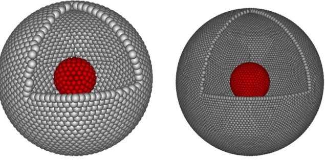
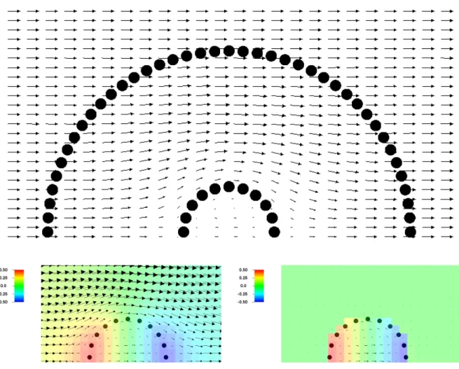
Figure 1: Two-dimensional Steady Stokes flow past a periodic column of circular cylinders (disks) at zero Reynolds number obtained using our rigid-body IB method (the same setup is also studied at finite Reynolds numbers in Section VII F). The markers used to mediate the fluid-body interaction are shown as small colored circles. The Lagrangian constraint forcesΛthat keep the markers at their fixed locations are shown as colored vectors; the color of the vectors and the corresponding marker iare based on the magnitude of the constraint forceΛi(see color bar). The fluid velocity field is shown as a vector field (black arrows) in the

vicinity and the interior of the body; further from the body, flow streamlines are shown as solid blue lines. The magnitude of the Eulerian constraint forceSΛis shown as a gray color plot (see greyscale bar). (Left panel) A volume marker grid of 121 markers is used to discretize the disk. The majority of the constraint forces are seen to act near the surface of the body, but nontrivial constraint forces are seen also in the interior of the body. (Right panel) A surface grid of 39 markers is used to discretize the disk, which strictly localizes the constraint forces to the surface of the body.

In the standard IB method for flexible immersed bodies, elastic forces are computed in the

Lagrangian frame and then spread to the fluid in the neighborhood of the markers using a regu-larized delta functionδa(r) that integrates to unity and converges to a Dirac delta function as the

regularization widtha→0. The regularization length scaleais typically chosen to be on the order

of the spacing between the markers (as well as the lattice spacing of the grid used to discretize the

fluid equations), as we discuss in more detail later. In turn, the motion of the markers is specified

to follow the velocity of the fluid interpolated at the positions of the markers.

the markers is known (e.g, they are fixed in place or move with a specified velocity) and the body

forces are unknown and must be determined within each time step. To obtain the fluid-marker

interaction forces Λ(t) = {Λi(t), . . . ,ΛN(t)} that constrain the motion of the N markers, we

solve for the Eulerian velocity fieldv(r, t), the Eulerian pressure fieldπ(r, t), and the Lagrangian

constraint forces Λi(t) the system

ρ(∂tv+v·∇v) +∇π=η∇2v+ N

X

i=1

Λiδa(Ri−r),

∇·v= 0,

Vi =

Z

δa(Ri−r)v(r, t) dr= 0, i= 1, . . . , N, (1)

along with suitable boundary conditions. In the case of steady Stokes flow, we setρ= 0. The first

two equations are the incompressible Navier-Stokes equations with an Eulerian constraint force

λ(r, t) =

N

X

i=1

Λiδa(Ri−r).

The last condition is therigidity constraintthat requires that the Eulerian velocity averaged around the position of marker i must match the known marker velocity Vi. This constraint enforces a

regularized no-slip condition at the locations of the IB markers, which is a numerical approximation

of the true no-slip condition on the surface (or interior) of the body. Observe that flow may still

penetrate the body in-between the markers and this leads to a well-known small but nonzero “leak”

in the traditional Peskin IB method. This leak can be greatly reduced by adopting a

staggered-grid formulation [44], as done in the present work. Other more specialized approaches to reducing

spurious fluxes in the IB method have been developed [45–47], but will not be considered in this

work.

Notice that for zero Reynolds number, the semi-continuum formulation (1) is closely related

to the popular method of regularized Stokeslets, which solves a similar system of equations for Λ

[21, 22]. The key difference 3 _{is that in the method of regularized Stokeslets, the fluid equations}

are eliminated using analytic Green’s functions; this necessitates that nontrivial pre-computations

of these Green’s functions be performed for each type of boundary condition [30, 31].

3

In this work, we treat (1) as the primary continuum formulation of the problem. This is a

semi-continuum formulation in which the rigid body is represented as a discrete collection of markers but

the fluid description is kept as a continuum, which implies that different discretizations of the fluid

equations are possible. One can, in principle, try to write a fully continuum formulation in which

the discrete set of rigidity forces Λ are replaced by a continuum force density field λ(R∈Ω, t).

The well-posedness and stability of such a fully continuum formulation is mathematically delicate,

however, and there can be subtle differences between weak and strong interpretations of the

equa-tions. To appreciate this, observe that if each component of the velocity is discretized with Nf

degrees of freedom, it cannot in general be possible to constrain the velocity strongly at more than

Nf points (markers). By contrast, in our strong formulation (1), the velocity is infinite dimensional

but it is only constrained in the vicinity of a finite number of markers. Therefore, the problem

(1) is always well posed and is directly amenable to numerical discretization and solution, at least

when it is well-conditioned. As we show in this work, the conditioning of the fully discrete problem

is controlled by the relationship between the regularization lengthaand the marker spacing.

The physical interpretation of the constraint forces Λi depends on details of the marker grid

and the type of the problem under consideration. For fully continuum formulations, in which the

fluid-body interaction is represented solely as a surface force density, the forceΛican be interpreted

as the integral of the traction (normal component of the fluid stress tensor) over a surface area

associated with markeri. Such a formulation is appropriate, for example, for steady Stokes flow. In

particular, for steady Stokes flow our method can be seen as a discretized and regularized first-kind

integral formulation in which Green’s functions are computed by the fluid solver. This approach

is different from the method of regularized Stokeslets, in which regularized Green’s functions must

be computed analytically [21, 22].

For cases in which markers are placed on both the surface and the interior of a rigid body,

the precise physical interpretation of the volume force density, and thus of Λ, is delicate even for

steady Stokes flow. Notably, observe that the splitting between a volume constraint force density

and the gradient of the pressure is not unique because the pressure inside a rigid body cannot be

determined uniquely. Specifically, only the component of the constraint force density projected

onto the space of divergence-free vector fields is uniquely determined. In the presence of finite

inertia and a density mismatch between the fluid and the moving rigid bodies, the inertial terms in (1) need to be modified in the interior of the body [35]. Furthermore, sufficiently many markers

in the interior of the body are required to prevent spurious angular momentum being generated

because they do not affect the numerical algorithm, and because we restrict our numerical studies

to flow past stationary rigid bodies, for which the fluid-body interaction force is localized to the surface of the body in the continuum limit.

III. DISCRETE FORMULATION

The spatial discretization of the fluid equation uses a uniform Cartesian grid with grid spacing

h and is based on a second-order accurate staggered-grid finite-difference discretization, in which

vector-valued quantities, including velocities and forces, are represented on the faces of the

Carte-sian grid cells, and scalar-valued quantities, including the pressure, are represented at the centers

of the grid cells [2, 35, 42, 43]. Our implicit-explicit temporal discretization of the Navier-Stokes

equation is standard and summarized in prior work; see for example the work of Griffith [43]. The

key features are that we treat advection explicitly using a predictor-corrector approach, and that

we treat viscosity implicitly, using either the backward Euler or the implicit midpoint method. For

steady Stokes flow, no temporal discretization required, although one can also think of this case as

corresponding to a backward Euler discretization of the time-dependent problem with a very large

time step size ∆t. A key dimensionless quantity is the viscous CFL number β =ν∆t/h2, where

the kinematic viscosity isν =η/ρ. Ifβ is small, the pressure and velocity are weakly coupled, but

for largeβ, and in particular for the steady Stokes limitβ → ∞, the coupling between the velocity

and pressure equations is strong.

We donot use a fractional time-stepping scheme (i.e., a projection method) to split the pressure and velocity updates; instead, the pressure is treated as a Lagrange multiplier that enforces the

incompressibility and must be determined together with the velocity at the end of the time step

[32]; except in special cases, this isnecessary for small Reynolds number flows. This approach also greatly aids with imposing stress boundary conditions [32]. The constraint forceλ(r, t) is treated

analogously to the pressure, i.e., as a Lagrange multiplier. Whereas the role of the pressure is to

enforce the incompressibility constraint,λ enforces the rigidity constraint. Like the pressure, λis

an unknown that must be solved for in this formulation.

A. Force spreading and velocity interpolation

In the fully discrete formulation of the fluid-body coupling, we replace spatial integrals by sums

is discretized using a tensor product ind-dimensional space (see [35] for more details),

δa(r) =h−d d

Y

α=1

φa(rα),

where hd is the volume of a grid cell. The one-dimensional kernel function φa is chosen based on

numerical considerations of efficiency and maximized approximate translational invariance [6]. In

this work, for reasons that will become clear in Section IV, we prefer to use a kernel that maximizes

translational and rotational invariance (i.e., improves grid-invariance). We therefore use the smooth

(three-times differentiable) six-point kernel recently described by Baoet al. [48]. This kernel is more expensive than the traditional four-point kernel [6] because it increases the support of the kernel to

62 = 36 grid points in two dimensions and 63 = 216 grid points in three dimensions; however, this

cost is justified because the new six-point kernel improves the translational invariance by orders of

magnitude compared to other standard IB kernel functions [48].

The interaction between the fluid and the rigid body is mediated through two crucial operations.

The discrete velocity-interpolation operator J averages velocities on the staggered grid in the

neighborhood of marker ivia

(Jv)α_i =X

k

vα_k φa(Ri−rαk),

where the sum is taken over faces k of the grid, α indexes coordinate directions (x, y, z) as a

superscript, andrα

k is the position of the center of the grid facek in the directionα. The discrete

force-spreading operatorS spreads forces from the markers to the faces of the staggered grid via

(SΛ)α_k =h−dX i

Λα_i φa(Ri−rαk), (2)

where now the sum is over the markers that define the configuration of the rigid body. These

operators are adjoint with respect to a suitably-defined inner product, J = S? = hdST, which

ensures conservation of energy [6]. Extensions of the basic interpolation and spreading operators

to account for the presence of physical boundary conditions are described in Appendix D.

B. Rigidly-constrained Stokes problem

At every stage of the temporal integrator, we need to solve a linear system of the form



   

A G −S

−D 0 0

−J 0 0

          v π Λ      =      g

h=0

W =0

which is the focus of this work. The right-hand side g includes all remaining fluid forcing terms,

explicit contributions from previous time steps or stages, boundary conditions, etc. Here, G is

the discrete gradient operator, D=−GT is the discrete divergence operator, andA is the vector

equivalent of the familiar screened Poisson (or Helmholtz) operator

A= ρ ∆tI−

κη h2Lv,

with κ = 1 for the backward Euler method or for steady Stokes, and κ = 1/2 for the implicit

midpoint rule. Here L_v is the dimensionless vector Laplacian operator, which takes into account

boundary conditions for velocity such as no-slip boundaries. Since the viscosity appears multiplied

by the coefficient κ, we will henceforth absorb this coefficient into the viscosity, η ← κη, which

allows us to assume, without loss of generality, that κ=1 and to write the fluid operator in the

form

A=ηh−2 β−1I−Lv

. (4)

We remark that making the (3,3) block in the matrix in (3) non-zero (i.e., regularizing the

saddle-point system) is closely related to solving the Brinkman equations [49] for flow through

a permeable or porous body suspended in fluid [4]. In particular, by making the (3,3) block a

diagonal matrix with suitable diagonal elements, one can consistently discretize the Brinkman

equations. Such regularization greatly simplifies the numerical linear algebra except, of course,

when the permeability of the body is so small that it effectively acts as an impermeable body. In

this work, we focus on developing a solver for (3) that is effective even when there is no regularization

(permeability), and even when the matrix Ais the discretization of an elliptic operator, as is the

case in the steady Stokes regime. This is the hardest case to consider, and a solver that is robust

in this case will be able to handle the easier cases of finite Reynolds number or permeable bodies

with ease.

It is worth noticing the structure of the linear system (3). First, observe that the system is

symmetric, at least if only simple boundary conditions such as periodic or no-slip boundaries are

present [32]. In the top 1×1 block,A_%0is a symmetric positive-semidefinite (SPD) matrix. The

top left 2×2 block represents the familiar saddle-point problem arising when solving the

Navier-Stokes or Navier-Stokes equations in the absence of a rigid body [32]. The whole system is a saddle-point

problem for the fluid variables and for Λ, in which the top-left block is the Stokes saddle-point

matrix.

C. Mobility matrix

We can formally solve (3) through a Schur complement approach, as described in more detail in

Section V. For increased generality, which will be useful when discussing preconditioners, we allow

the right hand side to be general and, in particular, do not assume thathand W are zero.

First, we solve the unconstrained fluid equation for pressure and velocity





A G

−D 0

    v π  =  

SΛ+g

h



, (5)

where we recall thatA=ηh−2 β−1I−L_v

. The solution can be written asv=L−1(SΛ+g) +

L−1_p h, whereL−1 is the standard Stokes solution operator for divergence-free flow (h= 0), given

by

L−1 =A−1−A−1G DA−1G−1

DA−1, (6)

where we have assumed for now thatA−1is invertible. For a periodic system, the discrete operators

commute, and we can write

L−1 =PA−1=

I−G(DG)−1DA−1, (7)

where P is the Helmholtz projection onto the space of divergence-free vector fields. We never

explicitly compute or formL−1; rather, we solve the Stokes velocity-pressure subsystems using the

projection-method based preconditioner developed by Griffith [32]. Let us define ˜v=L−1f+L−1_p h

to be the solution of theunconstrained Stokes problem





A G

−D 0

    ˜ v ˜ π  =   f h 

, (8)

giving v= ˜v+L−1SΛ.

Next, we plug the velocity v into the rigidity constraint,Jv=−W, to obtain

MΛ=−(W +Jv˜), (9)

where the Schur complement ormarker mobility matrix is

M=J L−1S =S?L−1S. (10)

The mobility matrixM_%0is SPD and has dimensionsdN×dN, and thed×dblockMij relates

efficient algorithm for the constraind fluid-solid system is to develop a method for approximating

the marker mobility matrix Min a simple and efficient way that leads to robust preconditioners

for solving the mobility subproblem (9); see Section IV.

Observe that the conditioning of the saddle-point system (3) is controlled by the conditioning

of M. In particular, if the (non-negative) eigenvalues of M are bounded away from zero, then

there will be a unique solution to the saddle-point system. If this bound is uniform as the grid

is refined, then the problem is posed and will satisfy a stability criterion similar to the

well-known Ladyzenskaja-Babuska-Brezzi (LBB) condition for the Stokes saddle-point problem (8). We

investigate the spectrum of the the marker mobility matrix numerically in Section V. In practice,

there may be some nearly zero eigenvalues of the matrixMcorresponding to physical (rather than

numerical) null modes. An example is a sphere discretized with markers on the surface: we know

that a uniform compression of the sphere will not cause any effect because of the incompressibility

of the fluid filling the sphere. This compression mode corresponds to a null-vector for the constraint

forcesΛ; it poses no difficulties in principle because the right-hand side in (9) is always in the range

ofM. Of course, when a discrete set of markers is placed on the sphere, the rotational symmetry

will be broken and the corresponding mode will have a small but nonzero eigenvalue, which can

lead to numerical difficulties if not handled with care.

D. Periodic steady Stokes flow

In the time-dependent context, β is finite, and it is easy to see thatA 0 is invertible. The

same happens even for steady Stokes flow if at least one of the boundaries is a no-slip boundary.

In the case of periodic steady Stokes flow, however, A = −ηh−2L_v has in its range vectors that

sum to zero, because no nonzero total force can be applied on a periodic domain. This means that

a solvability condition is

hSΛ+gi= vol−1

N

X

i=1

Λi+hgi= vol−11TΛ+hgi= 0,

where hi denotes an average over the whole system, 1 is a vector of ones, and vol is the volume

of the domain. This is an additional constraint that must be added to the constrained Stokes

system (3) for a periodic domain the steady Stokes case. In this approach, the solution has an

indeterminate mean velocity hvi because momentum is not conserved. This sort of approach is

followed for a scalar (reaction-diffusion) equivalent of (3) in the Appendix of Ref. [50], for the

Here, we instead impose the mean velocity hvi =0 and ensure that the total force applied to

the fluid sums to zero, i.e., we enforce momentum conservation. Specifically, for the special case of

periodic steady Stokes, we solve the system



   

A G − S−vol−11T

−D 0 0

−J 0 0

          v π Λ      =      g h W      , (11)

together with the constraint hvi=0, where we assume that hgi =0 for consistency. This change

amounts to simply redefining the spreading operator to subtract the total applied force on the

markers as a uniform force density, S ← S −vol−11T. This can be justified by considering the

unit cell to be part of an infinite periodic system in which there is an externally applied constant

pressure gradient, which is balanced by the drag forces on the bodies so as to ensure that the

domain as a whole is in force balance [51–53].

IV. APPROXIMATING THE MOBILITY MATRIX

A key element in the preconditioned Krylov solver for (3) that we describe in Section V is an

approximate solver for the mobility subproblem (9). The success of this approximate solver, i.e.,

the accuracy with which we can approximate the Schur complement of the saddle-point problem

(3), is crucial to an effective linear solver and one of the key contributions of this work.

Because it involves the inverse Stokes operator L−1, the actual Schur complement M =

S?L−1S cannot be formed efficiently. Instead of forming the true mobility matrix, we instead

approximate M≈Mf by a dense but low-rankapproximate mobility matrix Mf given by simple analytical approximations. To achieve this, we use two key ideas:

1. We ignore the specifics of the boundary conditions and assume that the structure is immersed

in an infinite domain at rest at infinity (in three dimensions) or in a finite periodic domain

(in two dimensions). This implies that the Krylov solver for (3) must handle the boundary

conditions.

2. We assume that the IB spatial discretization is translationally and rotationally invariant;

that is,Mdoes not depend on the exact position and orientation of the body relative to the

underlying fluid grid. This implies that the Krylov solver must handle any grid-dependence

The first idea, to ignore the boundary conditions in the preconditioner, has worked well in the

context of solving the Stokes system (8). Namely, a simple but effective approximation of the

inverse of the Schur complement for (8), DA−1G−1

, can be constructed by assuming that the

domain is periodic so that the finite difference operators commute, and thus the Schur complement

degenerates to a diagonal or nearly-diagonal mass matrix [32, 33, 54]. The second idea, to make

use of the near grid invariance of Peskin’s regularized kernel functions, has previously been used

successfully in implicit immersed-boundary methods by Ceniceroset al. [55]. Note that for certain choices of the kernel function, the assumption of grid invariance can be a very good approximation

to reality; here, we rely on the recently-developed six-point kernel [48], which has excellent grid

invariance and relatively compact support.

In the remainder of this section, we explain how we compute the entries in Mf in three

dimen-sions, assuming an unbounded fluid at rest at infinity. The details for two dimensions are given in

Appendix B and are similar in nature, except for complications for two-dimensional steady Stokes

flow resulting from the well-known Stokes paradox.

The mobility matrix M is a symmetric block matrix built from N ×N blocks of size d×d.

The blockMij corresponding to markersiandjrelates a force applied at markerj to the velocity

induced at marker i. Our basic assumption is that M_ij does not depend on the actual position

of the markers relative to the fluid grid, but rather only depends on the distance between the two

markers and on the viscous CFL numberβ in the form

f

M_ij =fβ(rij)I+gβ(rij) ˆrij⊗ˆrij, (12)

where rij = Ri −Rj and rij is the distance between the two markers, and hat denotes a unit

vector. The functions of distancefβ(r) andgβ(r) depend on the specific kernel chosen, the specific

discretization of the fluid equations (in our case the staggered-grid scheme), and the the viscous

CFL number β. To obtain a specific form for these two functions, we empirically fit numerical

data with functions with the proper asymptotic behavior at short and large distances between the

markers. For this purpose, we first discuss the asymptotic properties of fβ(r) and gβ(r) from a

physical perspective.

It is important to note that the true mobility matrixMis guaranteed to be SPD because of its

structure and the adjointness of the spreading and interpolation operators. This can be ensured

for the approximation Mf by placing positivity constraints on suitable linear combinations of the

Fourier transforms of fβ(r) and gβ(r), which ensure that the kernel M(ri,rj) given by (12) is

empirical fits in practice, and in this work, we do not attempt to ensureMf is SPD for all marker

configurations.

A. Physical Constraints

Let us temporarily focus on the semi-continuum formulation (1) and ignore Eulerian

discretiza-tion artifacts. The pairwise mobility between markersiand j for a continuum fluid is

Mij =η−1

Z

δa(Ri−r00)G(r00,r0)δa(Rj −r0) dr00dr0, (13)

where G(r,r0) is the the Green’s function for the fluid equation, i.e., v(r) = L−1f(r) =

R

G(r,r0)f(r0)dr0, where

ρ

∆tv+∇π−η∇

2_{v=f, (14)}

∇·v= 0.

It is well-known thatG has the same form as (12),

G(R1,R2) =f(r12)I+g(r12) ˆr12⊗rˆ12.

For steady Stokes flow (β → ∞), G ≡ O is the well-known Oseen tensor or Stokeslet 4, and

corresponds tofS(r) =gS(r)≈(8πηr)−1. For inviscid flow,β= 0, and we have thatA= (ρ/∆t)I

and (7) applies, and thereforeL−1 = (∆t/ρ)P is a multiple of the projection operator. For finite

nonzero values of β, we can obtain G from the solution of the screened Stokes (i.e., Brinkman)

equations (14) [23, 49, 56], and corresponds to the “Brinkmanlet” [23, 56]

fB(r) = e−αr

4πηr

1

αr

2 + 1

αr+ 1

!

− 1

4πηα2_r3, (15)

gB(r) =− e−αr

4πηr 3

1

αr

2 + 3

αr + 1

!

+ 3

4πηα2_r3,

whereα2 =ρ/(η∆t) = βh2−1

. Note that in the steady Stokes limit,α→0 and the Brinkmanlet

becomes the Stokeslet.

We can use (15) to construct Mf_ij when the markers are far apart. Namely, if r_ij h, then

we may approximate the IB kernel function by a true delta function, and thusfβ(r) andgβ(r) are

4

well-approximated by (15). For steady Stokes flow, the interaction between markers decays like

r−1. For finiteβ, however, the viscous contribution decays exponentially fast as exp −r/ h√β ,

which is consistent with the fact that markers interact via viscous forces only if they are at a

distance not much larger thanh√β =√ν∆t, the typical distance that momentum diffuses during

a time step. For nonzero Reynolds numbers, the leading order asymptotic r−3 decay offβ(r) and

gβ(r) is given by the last terms on the right hand side of (15) and corresponds to the electric field

of an electric dipole; its physical origin is in the incompressibility constraint, which instantaneously

propagates hydrodynamic information between the markers 5.

For steady Stokes flow, we can say even more about the approximate form of fβ(r) and gβ(r).

As discussed in more detail by Delong et al. [38], for distances between the markers that are not

too small compared to the regularization length a, we can approximate (13) with (12) using the

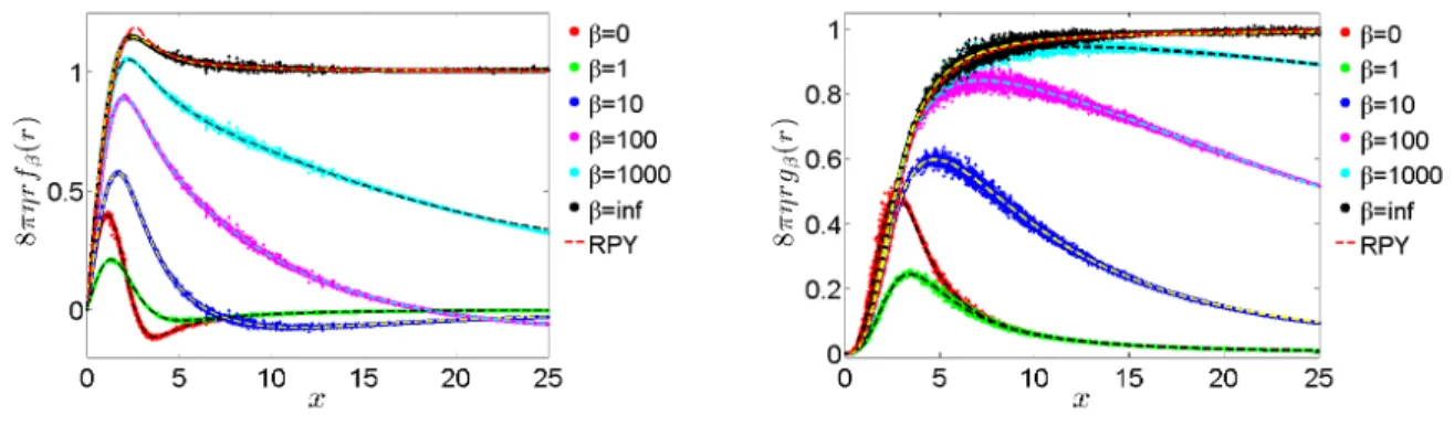
well-known Rotne-Prager-Yamakawa (RPY) [57–59] tensor for the functions fβ(r) and gβ(r),

fRP Y(r) =

1 6πηa

  

 

3a 4r +

a3

2r3, r >2a, 1−₃₂9r_a, r≤2a,

(16)

gRP Y(r) =

1 6πηa

  

 

3a 4r −

3a3

2r3, r >2a,

3r

32a, r ≤2a,

where a is the effective hydrodynamic radius of the specific kernel δa, defined by (6πa)−1 =

R

δa(r00)O(r00,r0)δa(r0) dr00dr0.Note that for r athe RPY tensor approaches the Oseen tensor

and decays like r−1. A key advantage of the RPY tensor is that it guarantees that the mobility matrix (12) is SPD forall configurations of the markers, which is a rather nontrivial requirement [59]. The actual discrete pairwise mobility Mij obtained from the spatially-discrete IB method

is well-described by the RPY tensor [38] (see Fig. 2). The only fitting parameter in the RPY

approximation is the effective hydrodynamic radius aaveraged over many positions of the marker

relative to the underlying grid [35, 38]; for the six-point kernel used here 6, a= 1.47h. For the

Brinkman equation, the equivalent of the RPY tensor can be computed for r ≥ 2a by applying

a Faxen-like operator from the left and right on the Brinkmanlet (see Eq. (26) in Ref. [56]); the

resulting analytical expressions are complex and are not used in our empirical fitting.

5

In reality, of course, this information is propagated via fast sound waves and not instantaneously.

6 _{As summarized in Refs. [35, 38], a ≈ 1.25h for the widely used four-point kernel [6], and a ≈ 0.91h for the}

B. Empirical Fits

In this work, we use empirical fits to approximate the mobility. This is because the analytical

approximations, such as those offered by the RPY tensor, are most appropriate for unbounded

domains and assume the markers are far apart compared to the width of the regularized delta

function. In numerical computations, we use a finite periodic domain, and this requires corrections

to the analytic expressions that are difficult to model. For example, for finite β, we find that

the periodic corrections to the inviscid (dipole) r−3 contribution dominate over the exponentially

decaying viscous contribution, which makes the precise form of the viscous terms in (15) irrelevant

in practice. For rh, only the asymptotically-dominant far-field terms survive, and we make an

effort to preserve those in our fitting because the numerical results are obtained using finite systems

and thus not reliable at large marker distances. At shorter distances, however, the discrete nature

of the fluid solver and the IB kernel functions becomes important, and empirical fitting seems to

be a simple yet flexible alternative to analytical computations. At the same time, we feel that is

important toconstrain the empirical fits based on known behavior at short and large distances. Firstly, for r h, the pairwise mobility can be well-approximated by the self-mobility (r = 0,

corresponding to the diagonal elementsMf_ii), for which we know the following facts:

• For the steady Stokes regime (β → ∞), the diagonal elements are given by Stokes’s drag

formula, yielding

f∞(0) = (6πηa)−1∼ 1/ηh and g∞(0) = 0,

where we recall that a is the effective hydrodynamic radius of a marker for the particular

spatial discretization (kernel and fluid solver).

• For the inviscid case (β = 0), it is not hard to show that [35]

f0(0) = d−1

d

∆t ρ V

−1

m ∼β/ηh andg0(0) = 0, (17)

whered= 3 is the dimensionality, and Vm=cVh3 is the “volume” of the marker, where the

constantcV is straightforward to calculate.

• The above indicates thatfβ(0) goes from ∼β/(ηh) for smallβ to∼1/(ηh) for largeβ. At

intermediate viscous CFL numbersβ, we can set

fβ(0) = C(β)

where C(β1) ≈2β/(3cV) is linear for small β and then becomes O(1) for large β. We

will obtain the actual form ofC(β) from empirical fitting.

Secondly, for rh, we know the asymptotic decay of the hydrodynamic interactions from (15):

• For the steady Stokes regime (β→ ∞), we have the Oseen tensor given by

f∞(r h)≈g∞(rh)≈(8πηr)−1. (19)

• For the inviscid case (β = 0), we get the electric field of an electric dipole,

f0(rh)≈ −

∆t

4πρr3 and g0(r h)≈

3∆t

4πρr3, (20)

which is also the asymptotic decay for β >0 for rh√β.

We obtain the actual form of the functions fβ(r) and gβ(r) empirically by fitting numerical data

for the parallel and perpendicular mobilities

µk_ij = ˆrT_ijMf_ijrˆ_ij ≈f_β(r_ij) +g_β(r_ij),

µ⊥_ij =rˆ⊥_ijT Mf_ijrˆ⊥_ij ≈f_β(r_ij),

where ˆr⊥_ij·ˆrij = 0. To do so, we placed a large number of markersN in a cube of lengthl/8 inside

a periodic domain of lengthl. For each markeri, we applied a unit forceΛi with random direction

while leavingΛj = 0 forj6=i, solved (8), and then interpolated the fluid velocityv at the position

of each of the markers. The resulting parallel and perpendicular relative velocity for each of the

N(N −1)/2 pairs of particles allows us to estimate fβ(rij) and gβ(rij). By making the number

of markersN sufficiently large, we sample the mobility over essentially all relative positions of the

pair of markers. For the self-mobility Mf_ii (r_ii = 0), we take g_β(0) = 0 and compute f_β(0) from

the numerical data.

If the spatial discretization were perfectly translationally and rotationally invariant and the

domain were infinite, all of the numerical data points for fβ(r) andgβ(r) would lie on a smooth

curve and would not depend on the actual position of the pair of markers relative to the underlying

grid. In reality, it is not possible to achieve perfect translational invariance with a kernel of finite

support [6], and so we expect some (hopefully small) scatter of the points around a smooth fit.

Normalized numerical data forfβ(r) andgβ(r) are shown in Fig. 2, and we indeed see that the data

can be fit well by smooth functions over the whole range of distances. To maximize the quality of the

Figure 2: Normalized mobility functions ˜f(x) (left) and ˜g(x) (right) defined similarly to (A1) as a function of marker-marker distance x=r/h, in three dimensions for the six-point kernel of Bao et al. [48], over a range of viscous CFL numbers (different colors, see legend). Numerical data is shown with symbols and obtained using a 2563 _{periodic fluid grid, while dashed lines show our empirical fit of the form (A2) for} steady Stokes (β → ∞) and (A6) for finiteβ. For steady Stokes flow, the numerical data is in reasonable agreement with the RPY tensor (16) (dashed red line).

make the fits change smoothly asβgrows towards infinity, as we explain in more detail in Appendix

A. Code to evaluate the empirical fits described in Appendices A and B is publicly available to

others for a number of kernels constructed by Peskin and coworkers (three-, four-, and six-point)

in both two and three dimensions at http://cims.nyu.edu/~donev/src/MobilityFunctions.c.

V. LINEAR SOLVER

To solve the constrained Stokes problem (3), we use the preconditioned flexible GMRES

(FGM-RES) method, which is a Krylov solver. We will refer to this as the “outer” Krylov solver, as it must

be distinguished from “inner” Krylov solvers used in the preconditioner. Because we use Krylov

solvers in our preconditioner and because Krylov solvers generally cannot be expressed as linear

operators, it is crucial to use a flexible Krylov method such as FGMRES for the outer solver. The

overall method is implemented in the open-source immersed-boundary adaptive mesh refinement

(IBAMR) software infrastructure [42]; in this work we focus on uniform grids and do not use the

AMR capabilities of IBAMR (but see [2, 41]). IBAMR uses Krylov solvers that are provided by

A. Preconditioner for the constrained Stokes system

In the preconditioner used by the outer Krylov solver, we want toapproximatelysolve the nested saddle-point linear system



   

A G −S

−D 0 0

−J 0 0

          v π Λ      =      g h W      ,

where we recall that A = (ρ/∆t)I−ηh−2Lv. Let us set α = 1 if A has a null-space, (e.g., for

a fully periodic domain for steady Stokes flow) and we set α = 0 if A is invertible. Whenα = 1,

let us define the restricted inverseA−1 to only act on vectors of mean value zero, and to return a

vector of mean zero.

Applying our Schur complement based preconditioner for solving (3) consists of the following

steps:

1. Solve the (unconstrained) fluid sub-problem,





A G

−D 0

    v π  =   g h  .

To control the accuracy of the solution one can either use a relative tolerance based stopping

criterion or fix the number of iterations Ns in the inner solver.

2. Calculate the slip velocity on the set of markers, ∆V =−(Jv+W).

3. Approximately solve the Schur complement system,

f

MΛ= ∆V, (21)

where the mobility approximation Mf is constructed as described in Section IV.

4. Optionally, re-solve the corrected fluid sub-problem,





A G

−D 0

    v π  =  

g+SΛ−αvol−11TΛ

h



.

All linear solvers used in the preconditioner can be approximate, and this is in fact the key to

the efficiency of the overall solver approach. Notably, the inner Krylov solvers used to solve the

of iterations using a method briefly described in the next section. If the fluid sub-problem is

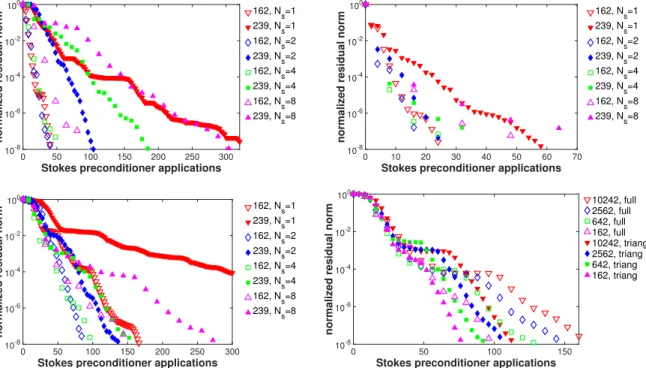
ap-proximately solved in both steps 1 and 4, which we term thefull Schur complement preconditioner, each application of the preconditioner requires 2Ns applications of the Stokes preconditioner (22).

It is also possible to omit step 4 above to obtain a block lower triangular Schur preconditioner [62], which requires onlyNs applications of the unconstrained Stokes preconditioner (22). We will

numerically compare these two preconditioners and study the effect of Ns on the convergence of

the FGMRES outer solver in Section VII A.

B. Unconstrained Fluid Solver

A key component we rely on is an approximate solver for the unconstrained Stokes sub-problem,





A G

−D 0

    v π  =   g h  ,

for which a number of techniques have been developed in the finite-element context [62]. To

solve this system, we use GMRES with a preconditioner P−1_S based on the projection method,

as proposed by Griffith [32] and improved to some extent by Cai et al. [33]. Specifically, the

preconditioner for the Stokes system that we use in this work is

P−1_S = 



I h2_G

f Lp

−1

0 Be

−1     I 0

−D −I



 

 e A−1 0

0 I



, (22)

where L_p =h2(DG) is the dimensionless pressure (scalar) Laplacian, andAe

−1

and Lf_p

−1

denote

approximate solvers obtained by a single V-cycle of a geometric multigrid solver for the vector Helmholtz and scalar Poisson problems, respectively. In the time-dependent case, the approximate

Schur complement for the unconstrained Stokes sub-problem is

e

B−1=−ρh 2

∆tLfp −1

+ηI,

and for steady Stokes flow,Be

−1

=ηI. Further discussion of the relation of these preconditioners

to the those described in the book [62] can be found in [32].

Observe that one application of P−1_S is relatively inexpensive and involves only a few scalar

multigrid V-cycles. Indeed, solving the Stokes system using GMRES with this preconditioner is

only a few times more expensive than solving a scalar Poisson problem, even in the steady Stokes

regime [33]. Note that it is possible to omit the upper right off-diagonal block in the first matrix on

and may in fact be preferred at zero Reynolds number since it allows one to skip a sweep of

the pressure multigrid solver [33]. We empirically find that including the Poisson solve (velocity

projection) improves the overall performance of the outer solver.

C. Mobility Solver

From a computational perspective, one of the most challenging steps in our preconditioner is

solving the mobility sub-problem (21). Since this is done inside a preconditioner, and because Mf

is itself an approximation of the true mobility matrixM, it is not necessary to solve (21) exactly.

In the majority of the examples presented herein, we solve (21) using direct solvers provided by

LAPACK. This is feasible on present hardware for up to around 105 markers and allows us to focus

on the design of the approximation Mf and to study the accuracy of the overall method.

Let us denote with s the smallest marker-marker spacing. For well-spaced markers, s/h ' 2,

our approximate mobility Mf is typically SPD even for large numbers of markers, and in these

cases, we can use the Cholesky factorization to solve (21). In some cases, however, there may

be a few small or even negative eigenvalues of Mf that have to be handled with care. We have

found that the most robust (albeit expensive) alternative is to perform an SVD of M, and tof

use a pseudoinverse of Mf (keeping only eigenvalues larger than some tolerance _{SV D} > 0) to

solve (21). This effectively filters out the spuriously small or negative eigenvalues. Note that

the factorization of Mf needs to be performed only once per constrained Stokes solve since the

body is kept fixed during a time step. In cases where there is a single body, the factorization

needs to be performed only once per simulation and can be reused; if the body is translating or

rotating, one ought to perform appropriate rotations of the right hand side and solution of (21).

In some cases of practical interest where the number of markers is not too large, it is possible

to precompute the true mobility M0 with periodic boundary conditions (for a sufficienly large

domain) and to store its factorization. Even if the structure moves relative to the underlying grid,

such a precomputed (reference) mobility M0 is typically a much better approximation to the true

mobility than our empirical approximation M, and can effectively be used in the preconditioner.f

Determining effective approaches to solving the mobility sub-problem in the presence of multiple

VI. CONDITIONING OF THE MOBILITY MATRIX

The conditioning of the constrained Stokes problem (3) is directly related to the conditioning

of the Schur complement mobility matrix M = J L−1S, which is intimately connected to the

relation between the fluid solver grid spacing h and the smallest inter-marker spacing s. Firstly,

it is obvious that if two markers iand j are very close to each other, then the fluid solver cannot

really distinguish between Λi and Λj and will instead effectively see only their sum. We also

know that using too many markers for a fixed fluid grid will ultimately lead to a rank-deficient

M, because it is not possible to constrain a finite-dimensional discrete fluid velocity at too many

points. This physical intuition tells us that the condition number of M should increase as the

marker spacing becomes small compared to the grid spacing. This well-known intuition, however,

does not tell us how closely the markers can or must be placed in practice. Standard wisdom for

the immersed boundary method, which is based on the behavior of models of elastic bodies, is to

make the marker spacing on the order of half a grid spacing. As we show, this leads to extremely

ill-conditioned mobility matrices for rigid bodies. We note that the specific results depend on the

dimensionality, the details of the fluid solver, and the specific kernel used; however, the qualitative

features we report appear to be rather general.

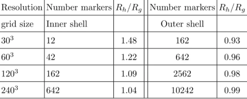
To determine the condition number of the mobility matrix, we consider “open” and “filled”

sphere models. We discretize the surface of a sphere as a shell of markers constructed by a recursive

procedure suggested to us by Charles Peskin (private communication). We start with 12 markers

placed at the vertices of an icosahedron, which gives a uniform triangulation of a sphere by 20

triangular faces. Then, we place a new marker at the center of each edge and recursively subdivide

each triangle into four smaller triangles, projecting the vertices back to the surface of the sphere

along the way. Each subdivision approximately quadruples the number of vertices, with thek-th

subdivision producing a model with 10·4k−1 + 2 markers. To create filled sphere models, we

place additional markers at the vertices of a tetrahedral grid filling the sphere that is constructed

using the TetGen library, starting from the surface triangulation described above. The constructed

tetrahedral grids are close to uniform, but it is not possible to control the precise marker distances

in the resulting irregular grid of markers. We use models with approximately equal edges (distances

between nearest-neighbor markers) of length≈s, which we take as a measure of the typical marker

spacing. We numerically computed the mobility matrixMfor an isolated spherical shell in a large

the marker spacing fixed ats≈1; one can alternatively keep the radius of the sphere fixed 7. In

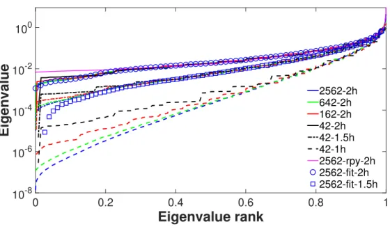
Fig. 3, we show the spectrum of Mfor varying levels of resolution for three different spacings of

the markers, s/h = 1, s/h = 3/2, and s/h = 2. Similar spectra, but with somewhat improved

condition number (i.e., fewer smaller eigenvalues), are seen for nonzero Reynolds numbers (finite

β).

The results in Fig. 3 strongly suggest that as the number of markers increases, the low-lying

(small eigenvalue) spectrum of the mobility matrix approaches a limiting shape. Therefore, the

nontrivial eigenvalues remain bounded away from zero even as the resolution is increased, which

implies that for s/h _& 1 the system (3) is uniformly solvable or “stable” under grid refinement.

Note that in the case of a sphere, there is a trivial zero eigenvalue in the continuum limit, which

corresponds to uniform compression of the sphere; this is reflected in the existence of one eigenvalue

much smaller than the rest in the discrete models. Ignoring the trivial eigenvalue, the condition

number ofMisO(N) for this example because the largest eigenvalue in this case increases like the

number of markersN, in agreement with the fact that the Stokes drag on a sphere scales linearly

with its radius. This is as close to optimal as possible, because for the continuum equations for

Stokes flow around a sphere, the eigenvalues corresponding to spherical harmonic modes scale like

the index of the spherical harmonic. However, what we are concerned here is not so much how the

condition number scales with N, but with the size of the prefactor, which is determined by the

smallest nontrivial eigenvalues of M.

Figure 3 clearly shows that the number of very small eigenvalues increases as we bring the

markers closer to each other, as expected. The increase in the conditioning number is quite rapid,

and the condition number becomesO(106−107) for marker spacings of about one per fluid grid cell.

For the conventional choice s≈h/2, the mobility matrix is so poorly conditioned that we cannot

solve the constrained Stokes problem in double-precision floating point arithmetic. Of course, if the

markers are too far apart then fluid will leak through the wall of the structure. We have performed

a number of heuristic studies of leak through flat and curved rigid walls and concluded thats/h≈2

yields both small leak and a good conditioning of the mobillity, at least for the six-point kernel

used here [48]. Therefore, unless indicated otherwise, in the remainder of this work, we keep the

markers abouttwo grid cells apart in both two and three dimensions. It is important to emphasize that this is just a heuristic recommendation and not a precise estimate. We remark that Taira and

7

Eigenvalue rank

0 0.2 0.4 0.6 0.8 1

Eigenvalue

10-8 10-6 10-4 10-2 100

2562-2h 642-2h 162-2h 42-2h 42-1.5h 42-1h 2562-rpy-2h 2562-fit-2h 2562-fit-1.5h

Figure 3: Eigenvalue spectrum of the mobility matrix for steady Stokes flow around a spherical shell covered with different numbers of markers (42, 162, 642, or 2562, see legend) embedded in a periodic domain. Solid lines are for marker spacing ofs≈2h, dashed-dotted lines for spacings≈1.5h, and dashed lines for spacing ofs≈1h. The marker spacing iss≈1 in all cases; fors≈2h, the fluid grid size is 1283 _{for 2562 markers} and 643for smaller number of markers, and scaled accordingly for other spacings. For comparison, we show the spectrum ofMfRP Y for the most resolved model (N = 2562 markers) at s/h ≈2. Also shown is the

spectrum of the empirical (fit) approximation to the mobilityMf for the two larger spacings; fors≈hour

empirical approximation is very poor and includes many spurious negative eigenvalues (not shown).

Colonius, who solve a different Schur complement “modified Poisson equation”, recommends/h≈1

to “achieve a reasonable condition number and to prevent penetration of streamlines caused by a

lack of Lagrangian points.”

It is important to observe that putting the markers further than the traditional wisdom will

increase the “leak” between the markers. For rigid structures, the exact positioning of the markers

can be controlled since they do not move relative to one another as they do for an elastic bodies;

this freedom can be used to reduce penetration of the flow into the body by a careful construction

of the marker grid. In the Conclusions, we discuss alternatives to the traditional marker-based IB

method [46] that can be used to control the conditioning number of the Schur complement and

allow for more tightly-spaced markers.

It is worthwhile to examine the underlying cause of the ill-conditioning as the markers are

nature of the fluid solver, which necessarily limits the rank of the mobility matrix. But another

contributor to the worsening of the conditioning is theregularization of the delta function. Observe that for a true delta function (a→0) in Stokes flow, the pairwise mobility is the length-scale-free

Oseen tensor ∼r−1, and the shape of the spectrum of the mobility matrix has to be independent of the spacing among the markers. In the standard immersed boundary method, a ∼ h, so the

fluid grid scaleh and the regularization scale aare difficult to distinguish.

To try to separate hfrom a, we can take a continuum model of the fluid, but keep the discrete

marker representation of the body; see (1). In this case the pairwise mobility would be given by

(13), which leads to the RPY tensor (16) for a kernel that is a surface delta function over a sphere

of radius a(see (4.1) in [59]). In Fig. 3 we compare the spectra of the discrete mobilityM with

those of the analytical mobility approximation Mf_{RP Y} constructed by using (16) for the pairwise

mobility. We observe that the two are very similar for s ≈ 2h, however, for smaller spacings

f

M_{RP Y} does not have very small eigenvalues and is much better conditioned than M(data not

shown). In Fig. 3 we also show the spectrum of our approximate mobility Mf constructed using

the empirical fits described in Section IV. The resulting spectra show a worsening conditioning for

spacing s ≈1.5h consistent with the spectrum of M. These observations suggest that both the

regularization of the kernel and the discretization artifacts contribute to the ill-conditioning, and

suggest that it is worthwhile to explore alternative discrete delta function kernels in the context of

rigid-body IB methods.

We also note that we see a severe worsening of the conditioning ofM, independent ofβ, when

we switch from a spherical shell to a filled sphere model. Some of this may be due to the fact that

the tetrahedral volume mesh used to construct the marker mesh is not as uniform as the surface

triangular mesh. We suspect, however, that this ill-conditioning is primarily physical rather than numerical, and comes from the fact that the present marker model cannot properly distinguish

between surface tractions and body (volume) stresses. Therefore, Λremains physically ill-defined

even if one gets rid of all discretization artifacts.

Lastly, it is important to emphasize that in the presence of ill-conditioning, what matters in

practice are not only the smallest eigenvalues but also their associated eigenvectors. Specifically,

we expect to see signatures of these eigenvectors (modes) in Λ, since they will appear with large

coefficients in the solution of (9) if the right hand side has a nonzero projection onto the

cor-responding mode. As expected, the small-eigenvalue eigenvectors of the mobility correspond to

high-frequency (in the spatial sense) modes for the forces Λ. Therefore, if the markers are too