Multi-camera simultaneous localization and mapping

(1)

MULTI-CAMERA SIMULTANEOUS LOCALIZATION AND MAPPING

Brian Sanderson Clipp

A dissertation submitted to the faculty of the University of North Carolina at Chapel Hill in partial fulﬁllment of the requirements for the degree of Doctor of Philosophy in the Department of Computer Science.

Chapel Hill 2010

Approved by:

Marc Pollefeys

Jan-Michael Frahm

Gary Bishop

Svetlana Lazebnik

Jongwoo Lim

(2)

c

2010

(3)

ABSTRACT

BRIAN SANDERSON CLIPP: Multi-Camera Simultaneous Localization and Mapping (Under the direction of Marc Pollefeys and Jan-Michael Frahm)

In this thesis, we study two aspects of simultaneous localization and mapping (SLAM) for multi-camera systems: minimal solution methods for the scaled motion of non-overlapping and partially overlapping two camera systems and enabling online, real-time mapping of large areas using the parallelism inherent in the visual simultaneous localization and map-ping (VSLAM) problem.

We present the only existing minimal solution method for six degree of freedom struc-ture and motion estimation using a non-overlapping, rigid two camera system with known intrinsic and extrinsic calibration. One example application of our method is the three-dimensional reconstruction of urban scenes from video. Because our method does not require the cameras’ ﬁelds-of-view to overlap, we are able to maximize coverage of the scene and avoid processing redundant, overlapping imagery.

Additionally, we developed a minimal solution method for partially overlapping stereo camera systems to overcome degeneracies inherent to non-overlapping two-camera systems but still have a wide total ﬁeld of view. The method takes two stereo images as its input. It uses one feature visible in all four views and three features visible across two temporal view pairs to constrain the system camera’s motion. We show in synthetic experiments that our method creates rotation and translation estimates that are more accurate than the perspective three-point method as the overlap in the stereo camera’s ﬁelds-of-view is reduced.

(4)

(5)

(6)

ACKNOWLEDGEMENTS

I would like to thank my advisor Marc Pollefeys and co-advisor Jan-Michael Frahm for their support of this work. There were times, particularly close to conference deadlines, that it seemed like some of the methods developed in this dissertation might not succeed. I am particularly grateful for Marc and Jan’s suggestions and encouragement at these times that helped me push through to solutions.

Thanks also to my committee members, Gary Bishop, Jongwoo Lim, Lana Lazebnik and Gregory Welch, who gave helpful advice and suggestions for this work.

My authors have been instrumental in completing this dissertation. This list of co-authors includes Richard Hartley, Jae-Hak Kim, Jongwoo Lim, Jan-Michael Frahm, Marc Pollefeys, Rahul Raguram, Gregory Welch, and Christopher Zach all of whom I would like to thank. Thanks in particular to Christopher Zach who helped me turn my geometric intuition into working algebraic solution methods. Also, thanks to Greg for the many in-teresting discussions we have had over the last few years. I am also grateful to Phillipos Mordohai, who as a post doc at UNC, along with Marc and Jan-Michael, helped me to gain my footing in multi-view geometry and computer vision.

My work in multi-camera systems involved building a lot of strange contraptions in-cluding a backpack mounted data collection system, a helmet mounted stereo camera, and a roof top recording platform for use on the department van. I owe a great deal of gratitude to John Thomas who built these systems that helped to make many of my experiments, whether presented in this dissertation or not, possible. Thanks John.

(7)

I have, and listening to my sometimes repetitive stories. I am going to miss our occasional procrastination sessions and mental breaks disguised as philosophical discussions.

Additionally, I would like to thank my family for their constant support and encourage-ment as I pursued my graduate studies. You all helped to keep me sane through this process by reminding me there are important things outside of academia.

(8)

LIST OF TABLES

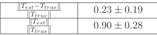
3.1 Relative translation vector error . . . 59

(12)

LIST OF FIGURES

1.1 Textured 3D models . . . 3

2.1 Basic VSLAM operations and data that passes between them . . . 8

2.2 Difference of Gaussian Kernel . . . 11

3.1 Multi-Camera System . . . 42

3.2 Overlapping and non-overlapping stereo cameras . . . 43

3.3 Two camera system motion . . . 45

3.4 Ray-plane intersection constraining scale . . . 48

3.5 Degeneracy due to rotation about a point . . . 50

3.6 Algorithm for scale estimation . . . 51

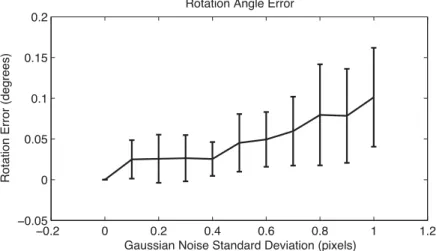
3.7 Rotation error, synthetic data . . . 54

3.8 Translation direction error, synthetic data . . . 55

3.9 Translation vector error, synthetic data . . . 55

3.10 Scale error, synthetic data . . . 56

3.11 Translation direction error, real data . . . 57

3.12 Rotation error, real data . . . 58

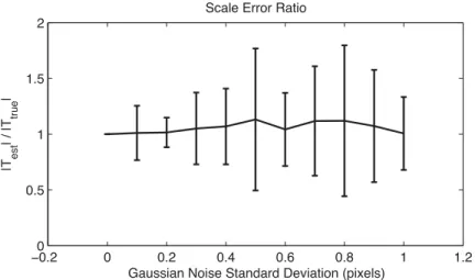
3.13 Scale ratio, real data . . . 58

3.14 Translation vector error, real data . . . 58

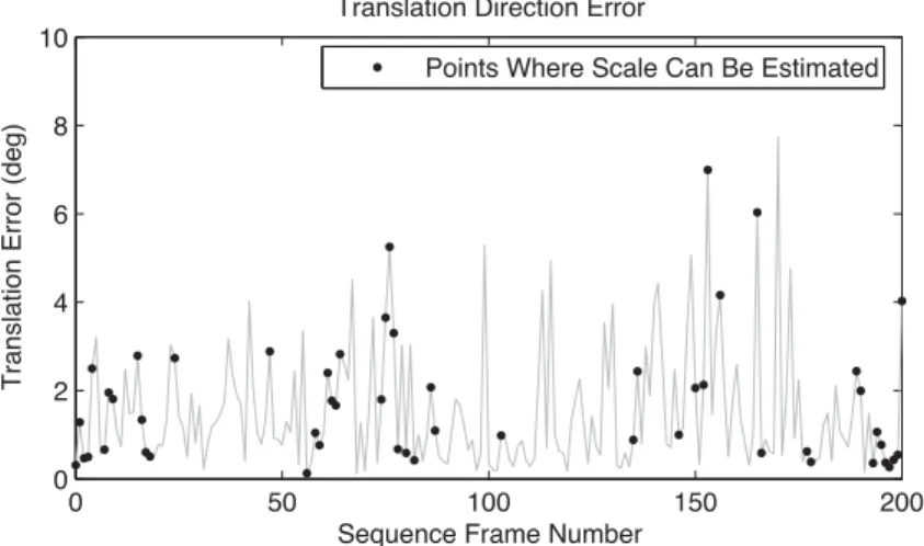
3.15 Locations where scale can be estimated in sequence . . . 60

3.16 Detected scale drift . . . 60

4.1 Geometry of partially overlapping stereo camera pose problem . . . 64

4.2 Minimal feature combinations for 6DOF stereo camera motion estimation . 73 4.3 Minimal solution method<1,1,1> . . . 75

(13)

4.5 First case of minimal solution method<0,2,2> . . . 76

4.6 Second case of minimal solution method<0,2,2> . . . 76

4.7 Line degeneracy . . . 77

4.8 Rotation, translation direction error, synthetic data . . . 80

4.9 Translation vector error, synthetic data . . . 81

4.10 Rotation error, synthetic data . . . 82

4.11 Translation direction error, synthetic data . . . 83

4.12 Scale error, synthetic data . . . 87

4.13 Visual odometry, ofﬁce scene from above . . . 88

4.14 Ofﬁce sequence sample frames . . . 89

5.1 System thread architecture . . . 92

5.2 Wide baseline matching using geometry from scene ﬂow features . . . 94

5.3 Sample frames from ofﬁce sequence . . . 103

5.4 Office sequence, top view with and without loop detection and correction . 104 5.5 Office sequence, side view with and without loop detection and correction . 105 5.6 Office sequence, overlaid on architectural layout . . . 106

5.7 Module timing . . . 107

5.8 Hallway sequence sample frames . . . 108

5.9 Loop detection and correction example . . . 109

5.10 Hallway sequence, results on architectural layout viewed from above . . . . 110

5.11 Hallway sequence, results viewed from side . . . 110

5.12 Error propagation through a bundle adjustment graph . . . 114

5.13 A single multi-grid V-cycle. . . 116

5.14 Possion heat equation solution grid . . . 117

5.15 An example random walk . . . 118

(14)

LIST OF ABBREVIATIONS

CCD Charge-Coupled Device

CUDA Compute Uniﬁed Device Architecture

DOF Degree of Freedom

DoG Difference of Gaussian

EKF Extended Kalman Filter

FAB-MAP Fast Appearance Based Mapping

fps Frames per Second

GNC Graduated Non-Convexity

GPU Graphics Processing Unit

GS Global SLAM

ICP Iterative Closest Point

KLT Kanade, Lukas, Tomasi feature tracker

LIDAR Light Direction and Ranging

MSER Maximally Stable Extremal Region

PTAM Parallel Tracking and Mapping

RANSAC Random Sample Consensus

SBA Sparse Bundle Adjustment

(15)

SfM Structure from Motion

SIFT Scale-Invariant Feature Transform

SLAM Simultaneous Localization and Mapping

TF-IDF Term-Frequency Inverse Document Frequency

VIP Viewpoint Invariant Patch

VO Visual Odometry

(16)

CHAPTER 1

Introduction

Visual Simultaneous Localization and Mapping (VSLAM) is the problem of using a mov-ing sensor system with one or more cameras to map an unknown environment and simul-taneously keep track of the sensor system’s pose within the map. The sensor system might be as simple as a single camera or could be a multi-camera system including other sensors such as accelerometers, gyroscopes, and wheel encoders. Like many problems in artiﬁcial intelligence VSLAM is something that most humans do fairly easily but is highly complex and difﬁcult to automate.

The more general simultaneous localization and mapping (SLAM) problem has been studied extensively in the robotics community (Kaess et al., 2007; Paskin, 2003; Thrun et al., 2005; Smith and Cheeseman, 1987). The sensors used in SLAM typically include Light Direction and Ranging (LIDAR), acoustic range sensors, bump sensors, as well as accelerometers, gyroscopes and wheel encoders. What sets apart visual SLAM is the use of cameras as sensors. In contrast to LIDAR, cameras are purely passive sensors and so do not emit any electromagnetic radiation. Because cameras are non-emissive, they typically require less power and are suitable for applications where stealth or a lack of interference between multiple systems is crucial. Additionally, cameras are less expensive than special-ized LIDAR sensors and are more pervasive in our world today. Most people today carry a mobile phone that includes a camera, which can be used for SLAM, as well as location recognition, which can support location-based services.

(17)

VSLAM problem a separate class of problem from general SLAM. Cameras provide bearing-only information, e.g. the direction to a target but not the distance to the target. Cameras also have effectively unlimited range; they detect the first object a ray encounters as it em-anates from the camera. In contrast, the range of LIDAR and acoustic sensors is limited by the amount of energy the sensor can broadcast into the environment and the reflectivity or absorbtion of the environment’s surfaces. This limited range actually simplifies the SLAM problem since only what is near the sensor can be measured by the sensor. This can lead to certain subdivisions of the map, which can simplify the SLAM problem. In contrast, the position of a camera system may have little to do with the spatial distribution of the objects it measures.

The VSLAM problem is important because it has applications in augmented reality, robotic navigation, remote sensing, and generating dense three-dimensional models from video. In augmented reality, a user views the world through some form of output device, generally either with a head-mounted display or hand-held device such as a cell phone. Synthetic objects are then placed on top of the real-scene in the user’s view. These objects could include information about the environment or synthetic game characters. In any case, to insert synthetic objects accurately, SLAM must be used to measure the pose of the display device in the environment. Visual SLAM (VSLAM) is an attractive option for augmented reality because of the low cost and power requirements of cameras and their relatively high angular resolution.

SLAM is also necessary for a robotic system to autonomously navigate its environment. It must have some way to create a map of its surroundings and measure its pose in the environment. The use of cameras in SLAM for robots is motivated by many of the same factors as in augmented reality. In particular, low power requirements can drive the choice of using VSLAM.

(18)

Figure 1.1: Textured 3D models reconstructed from multiple images.

video. Given the camera poses from VSLAM dense image matching can be performed to ﬁnd the depth of the scene with respect to the cameras, and given the camera poses the shape of the scene can be recovered in a global coordinate frame. Once the scene shape is recovered, it can be textured with the imagery to create visually appealing virtual models of the measured environment. Some example models are shown in Figure 1.1.

(19)

CHAPTER 2

The Visual SLAM Problem

The “Visual SLAM” problem, which is also known as “Structure from Motion”, has been studied extensively in the robotics and computer vision ﬁelds. This chapter will give a brief history of the VSLAM problem as well as introduce the state of the art in VSLAM. It will then discuss the structure of the VSLAM problem and the various sub-processes that must be done in any VSLAM system namely, correspondence ﬁnding, relative pose estimation, and global mapping.

Harris and Pike demonstrated one of the ﬁrst VSLAM methods on an image sequence (Harris and Pike, 1988). Their work contained many of the major components of a VSLAM system including feature matching, relative pose estimation, and a Kalman ﬁlter based method for fusing the measurements from multiple views. Using a stereo camera, their system created a map of point and line features with covariance matrices representing their uncertainties. However, they neglected the correlations between features which can create problems.

(20)

and when we ﬁnally see the window reject it’s features as outliers.

Another area where correlations are critical is in loop completion. Consider the simple case were a camera is panned around the vertical so that it views the walls of a room. As it turns it builds a map of the walls and its pose. The farther it turns away from the origin (its starting pose) the more uncertain its pose is as well as its feature estimates. When the camera turns all the way around and re-detects features that were mapped in the ﬁrst image this completes a loop. Recognizing that the features at the end of the loop are the same as those at the beginning should reduce the uncertainty of the features seen in the frames just before the loop was completed as well as update their positions. Without modeling the correlations between features this update is impossible and the loop cannot be properly completed. As stated by Davison (2007), ignoring the correlations between features could lead to over-conﬁdence in the feature estimates’ accuracy and the inability to close loops or detect drift.

Azarbayejani and Pentland presented an Extended Kalman Filter (EKF) approach to recursively estimate the structure, camera motion and camera focal length from an image sequence (Azarbayejani and Pentland, 1995). Davison (2007) was the first to demonstrate a real-time VSLAM system using a single camera as its only measurement device. His work was also based on an Extended Kalman Filter and could map areas the size of a desktop or small room, detecting and completing loops. Davison’s system modeled the correlations between mapped features. This made the filter’s estimate of uncertainty consistent, but it limited the number of features that could be mapped in real time to less than one-hundred. A particle filter approach to VSLAM was presented by Eade and Drummond (2006). Their system could also map small office scale environments but the small number of par-ticles that could be processed in real time limited their map size.

(21)

Euclidean maps connected by transformations. Since each Euclidean map is limited in size it can be updated in real-time. A major drawback of this approach is that global correction is done by ﬁxing the sub-maps and varying the transformations between them. This forces all of the error accumulated in each of the sub-maps into the joints between the maps.

Eade and Drummond (2007) used a sub-map based approach to accelerate the mapping process in. In their work, each sub-map contained about ﬁfty 3D features with their associ-ated uncertainties and correlations stored in a covariance matrix. They used the Laplacian of the projection function as a measure of the non-linearity of the projection function in or-der to decide where to split the map into sub-maps. By limiting the sub-map sizes they can fold the information from a new image into the map in real-time. Additionally, they can op-timize the sub-maps with respect to each other to arrive at a globally consistent map. This is critical because inconsistency can lead to problems in detecting and correcting loops.

(22)

The VSLAM method presented in Chapter 5 differs from PTAM in that we can explore new areas while the map is globally corrected. In PTAM new key-frames can only be added between global map corrections, limiting the rate of key-frame addition as the map grows. In our method global map correction must complete between new loop completions rather than between new key-frames, signiﬁcantly increasing the size of areas that can be mapped online and in real-time.

Scalability of performance to larger map sizes was a focus of Konolige and Agrawal’s method called “FrameSLAM” (2008). Like Klein and Murray, they also used selected key-frames from the image sequence and only included these in the map. Konolige and Agrawal’s innovation was to convert the constraints imposed by corresponding feature mea-surements in two images into a synthetic measurement with an associated uncertainty tying the two camera poses together with a sort of virtual spring. This permanently marginalizes out the features from the map, signiﬁcantly speeding up the minimization used to correct for loops in the camera’s path. Their method achieves this speedup at the cost of a less accurate map structure. Accuracy is reduced because the feature measurements cannot be re-linearized once the features are permanently marginalized out of the optimization.

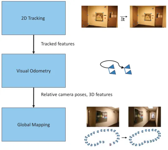
2.1 Basic Structure of the VSLAM Problem

(23)

2D Tracking

Visual Odometry

Global Mapping

Tracked features

Relative camera poses, 3D features

∆t

Figure 2.1: Basic VSLAM operations and data that passes between them

and discuss relevant prior work.

(24)

2.2 Correspondence Finding

There are two major types of correspondence finding approaches: unguided approaches that find correspondences without modeling inter-correspondence relationships, and those guided by and coupled to 3D relative camera pose estimation. Unguided approaches were the first to be developed by the computer vision community so they will be described first.

2.2.1 Unguided Correspondence

Unguided correspondence methods estimate optical ﬂow without any camera motion model or other external sensors, e.g. inertial sensors. Unguided approaches can be roughly divided into two classes: differential-tracking approaches that depend on a small feature motion assumption, and matching approaches that can ﬁnd correspondence in pairs of images with larger viewpoint changes.

(25)

Many approaches exist for ﬁnding feature correspondences over wide baselines. Harris features (Harris and Stephens, 1988) are extracted at strong corners in the image as mea-sured by the gradient magnitude in a local region. Harris corners use an approximation to the eigenvalues of the structure tensor to detect features. For this reason, they give a less accurate response than Tomasi and Shi’s operator (1994) but are more computationally efﬁcient.

One of the limitations of Harris features is that they are point features, lacking an in-trinsic scale or neighborhood size. Lowe (2004) showed how a scale space approach to detecting blob-like features using convolution with a difference of Gaussian (DoG) oper-ator could lead to scale invariance. The difference of Gaussian operoper-ator is an approxima-tion to the Laplacian of Gaussian operator and so reacts strongly to blobs. The equaapproxima-tion f(x) = _2Π1_σ2exp

−x2

2σ2

− 1

2ΠK2σ2exp

−x2

2K2σ2

describes a DoG filter kernel. In that equa-tionxis the position with respect to the filter origin,σis the filter’s standard deviation and K is a scaling factor tuned to make the DoG best approximate the Laplacian of Gaussian. An example DoG filter is shown in Figure 2.2 withK = 1.6and σ = 1.0. Lowe’s SIFT feature (2004) combines the scale space blob detection with patch orientation based on gradient magnitude and a descriptor based on a histogram of gradients to achieve corre-spondence between images at up to a thirty-degree change in viewing angle.

(26)

−10 −5 0 5 10 −0.02

0 0.02 0.04 0.06 0.08 0.1

Difference of Gaussian Function

Distance From Mean

Filter Response

Figure 2.2: A one-dimensional Difference of Gaussian kernel.

al. demonstrated an extraction method that wasO(nlog(log(n)))wherenis the number of pixels in the image. Later Nist´er and Stew´enius (2008) showed that MSER features can be extracted with an algorithm that is at worstO(n).

Each of the preceding feature extraction methods extracts features in each frame ind-pendently and without regard for the correlations between feature positions that can come from an underlying model of the scene geometry and camera motion. The following section will introduce guided correspondence ﬁnding methods that make use of this correlation to improve matching.

2.2.2 Guided Correspondence

(27)

the search area for correspondences. A reﬁnement is then performed starting at these pre-dicted feature locations to ﬁnd the features. The advantage of this framework is that it can handle faster camera dynamics than a differential feature tracker, can cope to some extent with repetitive features, and is less computationally expensive than many feature extraction methods.

This search-based approach does not take into account how informative a given feature is about the camera pose. Davison (2005) shows that the mutual information between the map state (3D feature positions and camera pose with uncertainties) and the measurements can determine how much information is gained by finding a given feature. This expected information gain can then be combined with the cost of detecting that feature to determine the relative efficiency in terms of information gain per unit computational cost of detecting a feature. Features can then be found in the most informative order. As each feature is found, it also reduces the uncertainty of the other features, which reduces the computational cost of finding those features. Given a fixed time budget, ordering by relative information efficiency gives the most information about the map state possible.

(28)

many more features in real time than were possible with a dense measurement covariance matrix.

2.3 Relative Pose Estimation

Relative pose estimation is the process of calculating the rotation and translation of a cam-era or multi-camcam-era system from two sets of images taken at two different times. Relative pose estimation methods can be broken up into two primary classes: those that use sparse feature correspondences as their input, and those that rely on dense optical ﬂow. The for-mer are much more commonly used in practice. An example of the latter, dense optical ﬂow based method, was introduced in (Yang et al., 2007).

Relative pose methods that use sparse feature correspondences can further be broken into two classes, those that use a predictive motion model, and those that do not. A predic-tive motion model is generally a very simple assumption on the camera motion such as, ”the camera moves with constant velocity.” Filtering approaches to visual SLAM (Azarbayejani and Pentland, 1995; Davison et al., 2007; Eade and Drummond, 2006) use a predictive motion model which, in combination with the expected 3D position of the sparse features based on a static world model and their uncertainties, gives a search region in the current frame for previously mapped features. Once these features are found, the pose estimate can be reﬁned starting from the predicted pose.

(29)

Relative pose estimates that do not use a predictive motion model generally rely on ran-dom sampling of correspondences between features in the current image and either another image or 3D features in the map itself. This random sampling and consensus (RANSAC) approach was ﬁrst introduced by Bolles and Fischler in (Bolles and Fischler, 1981). The basic RANSAC algorithm for relative pose is given in Algorithm 1.

Data: Set of putative correspondences C

Result: Relative poseP_iand inlier correspondencesC_in conﬁdence in having seen a good solution = 0;

best sample support = 0;

whileconﬁdence in having seen a good solution<thresholddo select a minimal set of correspondences;

use minimal set of correspondences to calculate relative pose; test whether or not correspondences support solution;

ifcurrent sample support>best sample supportthen best sample = current sample;

best sample support = current sample support;

end

calculate conﬁdence in having seen a correct solution;

end

Algorithm 1:The RANSAC algorithm applied to relative pose estimation

(30)

taken so far. p_incan be taken from the inlier ratio of the best solution found yet in the data. The interplay of the inlier ratio p_in and the number of samples determines the number of random samples that must be drawn to generate an output from the RANSAC algorithm with an acceptable level of conﬁdencec(solution). This means that with low inlier ratios, p_in, a large number of samples may be required to get a solution with a desired level of conﬁdence. Unfortunately, this means that unless some a priori bound can be given on the inlier ratio, the sampling time is not bounded and so RANSAC cannot be used in a hard-real-time system.

Many optimizations to RANSAC have been suggested (Nistér, 2003; Raguram et al., 2008) but none has overcome this fundamental flaw in RANSAC. Given a fixed time budget these methods will return the least bad solution they can find. However, the confidence in that solution may be too low for the solution to be used in practice if a lower bound on the inlier ratio is not given.

The RANSAC algorithm returns the best minimal sample solution found as well as the set of inliers. To get a more accurate solution, a refinement of the solution should be performed using all of the inlier correspondences. Even the best solution after RANSAC is still based only on a small set of correspondences which themselves contain some amount of noise. Assuming the noise on the inliers is normally distributed, refinement with a larger set of inlier correspondences will arrive at a more accurate result. This refinement can be done with a simple linear method or a more complicated non-linear minimization may be required.

2.4 Direct Solution Methods

(31)

spe-cific problem such as homography estimation (Brown et al., 2007; Horn, 1987), motion estimation for calibrated monocular cameras (Nistér, 2003), uncalibrated monocular cam-eras (Hartley and Zisserman, 2004), multi-camera systems (Clipp et al., 2008; Kim et al., 2007) or generalized camera approaches (Stewénius et al., 2005).

Each direct solution method is typically formulated as a problem of algebraic geometry and then solved using a unique method of the author’s choosing. Recently, Kukelova et al. (2008) have developed a method to automatically generate minimal problem solvers. Careful consideration must be given to numerical performance in a direct solver, as this can greatly inﬂuence the reliability of the solver’s result. Additionally some solution meth-ods are based on ﬁnding the roots of a polynomial function. Each of these roots must be tested in the RANSAC framework as a separate possible solution and so the degree of the polynomial also has a great impact on performance.

This dissertation focuses on visual SLAM for rigid multi-camera systems and so some background on direct solution methods for these systems is in order. Nistér’s seminal work on visual odometry (2004) used the perspective three-point (P3P) method (Haralick et al., 1994) to generate relative pose samples. The P3P method uses correspondence between an image from a calibrated camera and a set of 3D point features to find the pose of the camera with respect to those features. In Nistér’s case he built a map of 3D point features as he moved the camera, enabling him to estimate the next camera pose with respect to the existing map. His verification in RANSAC was then done with correspondences from both cameras in his system’s rigid stereo head.

(32)

A particularly challenging problem is to develop a method to calculate the six degree of freedom motion of a non-overlapping multi-camera system. Weng and Huang (1992) pre-sented one of the earliest works in this area. In their work they described how this motion could be calculated using a non-minimal linear equation and described motions that could lead to degenerate solutions algebraically. Their equations allow for the non-overlapping multi-camera system’s extrinsic calibration to change between images. However, this cali-bration must be known at each frame.

Dornaika and Chung (2003) extended the work of Weng and Huang (1992) by showing that a non-overlapping multi-camera system could be calibrated up to an unknown scale factor without stereo correspondence. Their method uses a three-stage process. First, the ego-motion of each camera is calculated separately. These ego-motions are then combined to calculate the relative orientation between the multi-camera system’s cameras. Finally, the relative scaling between the motions of the various cameras is found, placing each of the cameras in a single arbitrarily scaled coordinate frame.

Frahm et al. (2004) also developed a pose estimation method for multi-camera systems with non-overlapping ﬁelds of view. Theirs is a linear but non-minimal approach. Interest-ingly, when applying their equations to model a single camera system the equations reduce to the linear single camera pose estimation method with respect to a known set of homoge-nous world features given in (Hartley and Zisserman, 2004). Frahm et al. also develop a method to automatically calibrate a multi-camera system up to an unknown scale factor from correspondences. In contrast to Dornaika and Chung (2003), the calibration method of Frahm et al. requires overlap in the cameras’ ﬁelds of view.

(33)

estimation using the known geometry of the multi-camera system to ﬁnd the absolute scale of the scene and motion without stereo correspondence. Kim and Chung also point out that adding a simple rotation of the multi-camera system about a single axis as the rig is moved can prevent degenerate motions in almost all practical cases.

Kim et al. (2007) have also solved the problem of 6DOF motion estimation by formu-lating it as a triangulation problem. They ﬁrst solve for the rotation of the multi-camera sys-tem by averaging the rotations measured by each of the cameras independently. They then triangulate the translation directions of the system’s cameras to arrive at a scaled measure of the camera system’s translation. They use a second order cone programming approach for triangulation, which is optimal in the L-Inﬁnity norm. Since it requires 5DOF motion estimates for each of the cameras to calculate the scaled motion, theirs is a non-minimal solution method.

Tariq and Dellaert (2004) have also developed a method for estimating the pose of a multi-camera system. Their method uses a non-linear minimization of the reprojection error of known 3D features. Using synthetic data, they show that increasing the number of cameras in a multi-camera system can improve the rotation and translation estimation accuracy, and prevent catastrophic failures due to a lack of tracked features.

Ni and Dellaert (2006) developed a method for six degree of freedom stereo camera motion estimation based on decomposing the problem into estimating the rotation from points at inﬁnity followed by the translation. Their method assumes an initial starting point close to the true motion solution, and then performs a non-linear minimization to ﬁnd the rotation, and then translation in a two-stage approach. Assuming an initialization as they do is appropriate for applications processing video sequences but cannot be used on general photo collections.

(34)

rays can intersect at any number of optical centers with each ray possibly having its own optical center. A generalized camera can be used to model any camera or multi-camera system. Nist´er’s (2004) generalized three-point solution method is based on a generalized camera model, hence its name.

Stewénius et al. (2005) presented a minimal solution method for estimating the six degree of freedom motion of a generalized camera from image correspondences. They showed that there are up to sixty-four solutions to the relative pose of two generalized cameras given six ray correspondences. One of the limitations of their approach is that it is degenerate for generalized cameras where the rays’ centers of projection are all on a line. This naturally excludes all two-camera systems, as two camera centers always form a line. Chapter 3 will describe one of the contributions of this dissertation, a novel six degree of freedom relative pose estimation method for a non-overlapping rigid two camera system using a minimal set of six correspondences. Using a system of two or more non-overlapping cameras, scene coverage can be maximized with this method while still measuring the true scale of the motion. In Chapter 4, another contribution of this dissertation is described. This is a method for estimating the scaled, six degree of freedom motion of a stereo camera with only a small overlap in the cameras’ fields-of-view. This novel method overcomes some of the limitations of the method introduced in Chapter 3 while still giving the multi-camera system a large total field of view.

(35)

2.5 Global Mapping

In this dissertation, global mapping refers to the processes that a SLAM system must per-form to create an internal representation of its operating environment when all of the en-vironment is not visible from a single point of view. At a minimum, the global map must reﬂect the topology of the operating environment, i.e. the connectivity between the various parts of the environment. This requires that the VSLAM system performloop detection.

However, for many practical applications, a topological map is not enough and a Eu-clidean map is required. Some example applications where a EuEu-clidean map is required are efﬁcient path planning and automated targeting. A Euclidean map is the sort of map we are generally accustomed to where each point on the map is known with respect to every other point and the map has a single scale. Additionally, in a Euclidean map distances and angles are preserved. When creating a Euclidean map it is not simply enough to make note of a loop when it is detected. The system must also performloop correction to make the geometry of the map reﬂect the Euclidean geometry, not just the topology, of the operating environment. Additionally, the global geometry of a Euclidean map can help to eliminate false loop detections. For example, when mapping a building by moving around it, if two corners of a building look the same and have similar geometry, we can use the shape of the path taken around the building to disambiguate the corners.

2.5.1 Loop Detection

(36)

Sivic and Zisserman (2003) were the first to apply text retrieval techniques to find ob-jects within a video sequence. Their approach is suitable for loop detection since it finds images with common structure in a video sequence. They use both SIFT descriptors (Lowe, 2004) and maximally stable extremal regions (MSER) (Matas et al., 2002). Their approach consists of a preprocessing step followed by a retrieval phase. In the preprocessing step SIFT and MSER features are extracted in each of the images. A subset of these image’s features are then grouped using K-means clustering. Each of these clusters is referred to as a visual word. They use approximately 500 images in the clustering and generate ap-proximately 10000 distinct visual words. They are limited in the number of clusters they can generate by the complexity of K-means clustering with such a large number of clus-ters. Each image’s features are then quantized into visual words. An inverted file is stored for each visual word, which contains which images a visual word is found within and the visual word’s position in that image.

When querying to find an object in the video the user selects a region of interest con-taining this object. The system then finds the descriptors in this region and their visual words. It then uses a term-frequency inverse document frequency (TF-IDF) weighting for-mula to find other images in the video that contain the same visual words. The TF-IDF weighting takes into account both the frequency of a given visual word in the current im-age and the log inverse frequency of a visual word in the documents. The TF-IDF formula ist_i = nid

nd log

N

ni wherenid is the number of occurrences of visual wordiin documentd, n_dis the total number of visual words in documentd,N is the number of documents in the database andn_i is the number of documents containing visual wordi.

Each document in the database (video) is represented by a vector of TF-IDF values for each visual word:

(37)

The dot products of the vector representing the query region and each document in the database can then be taken to find images that are likely to contain the object of interest. The method then performs a final geometric verification step. Their method starts with two matched feature regions and looks at the local neighborhood of each feature. The same features in the local neighborhood of the matched features should be found in both frames. This is a form of loose geometric verification, which does not enforce any sort of global model such as a homography or essential matrix.

Sivic and Zisserman show that their system vastly out-performs this naive approach in terms or run time as well as precision-recall curves. The improvement in precision and recall is primarily due to the TF-IDF weighting of the descriptors and their weak geometric veriﬁcation.

Nistér and Stewénius (2006) extended the work of Sivic and Zisserman in image re-trieval. Their vocabulary tree approach uses a hierarchical k-means clustering of the feature space to partition features into visual words. The tree-based approach overcomes scaling issues that limited the vocabulary size in Sivic and Zisserman (2003). With a larger number of visual words, the descriptor space can be broken up into more discriminative, smaller clusters. A larger number of smaller clusters improve image retrieval performance. Addi-tionally, because their visual words were more discriminative, Nistér and Stewénius found that they did not need to use geometric verification to achieve good performance. They show results on up to a one-million image database, three orders of magnitude larger than Sivic and Zisserman’s results.

(38)

train-ing data, reflects the fact that certain visual words are likely to co-occur in an image because they come from the same object. Knowing which features are likely to appear or disappear together because they are part of the same object or objects, the system in effect recognizes unique locations by finding unique groupings of objects in the imagery. The system also recognizes which visual words appear in many locations because of repetitive scene parts. This is known as perceptual aliasing. In Nistér and Stewénius’s approach, perceptual alias-ing is handled by the inverse document frequency term while in Cummins and Newman’s model a probabilistic approach is taken.

Cummins and Newman make a comparison between a naive Bayesian assumption that the likelihood of a visual word being found in an image is independent of the other visual words in the image and a model that takes into account the correlations between visual word occurrences. They show that using a simplification of the full correlation between all features based on a Chow Liu tree (Chow and Liu, 1968) can provide significant perfor-mance improvements over the naive Bayesian approach at little additional computational cost. The Chow Liu tree is a maximal spanning tree over the correlation between features which, while it is a simplification over the full correlation matrix, provides good perfor-mance with close to real-time computation.

(39)

way, the information from one feature match can reduce the pose uncertainty and therefore limits the search region size for subsequent features. In later work, they developed more efﬁcient methods to represent the probabilistic constraints between the feature projections (Ankur Handa and Davison, 2010). These methods make real-time probabilistic feature matching possible.

Geometry-ﬁrst methods have been successfully demonstrated on small room-sized en-vironments. However, were they to be used in mapping larger environments, the large uncertainty in the camera pose prior after traveling long distances would become an issue. With a large pose uncertainty, such as one would have after traversing a large loop, the projection of the feature uncertainty regions in the image would be extremely large. Also, the number of features that might project in the image grows as the camera may take on a wide range of poses. A more efﬁcient approach is needed.

Appearance-first approaches can detect loops of any size because they do not rely on a camera pose prior. In the work of Irschara et al. , a vocabulary tree (Nistér and Stewénius, 2006) and inverted files are used to find visually similar parts of a database of images. These images have been previously processed into a 3D point cloud model of the environ-ment. Features are then matched between the query image and the map based on descriptor similarity (dot product of SIFT features). The perspective three-point method (Haralick et al., 1994) in a RANSAC framework is then used to verify that the geometry of the scene could indeed generate the feature distribution in the query image. However, Irschara et al. do more than just this. They create virtual views of the 3D point cloud model and use these as the database that query images are compared with. This significantly reduces the num-ber of images in the database, speeding up the histogram generation from the inverted files. They also make extensive use of the graphics processing unit (GPU) to speed up processing query image features into visual words through the vocabulary tree.

(40)

Williams et al. (2007). Their approach, which they call ferns, uses a collection of simple Bayesian classifiers to separate key-points into a set of classes. These classifiers (ferns) start with an image patch representing the key-point. Each classifier is then made up of a set of binary decisions. Two pixels are randomly selected in the patch and if one pixel is brighter than the other the value is one, otherwise the binary decision value is zero. Using a large number of these random binary measurements over the image patch a distribution of resulting binary numbers (fern results) can be found over a large training set of examples of the same image patch. These examples can be synthetically generated affine warps of an original image patch. In practice the number of binary decisions (leaves in the fern) must be large (L = 300) to achieve acceptable classification performance. For each key-point, the method must calculate the probability that it takes on any one of the2300possible fern output values. This is intractable and so the authors simplify the computation by breaking up the large fern into M smaller ferns each of which can take on 2L/M values. The classification results of this group of ferns are then multiplied together to form the final probability of a feature being of a particular class. Grouping the binary decisions into small ferns performs better experimentally than assuming that each of the binary decisions is statistically independent.

Ferns were an outgrowth of and an improvement on Lepetit and Fua’s work on ran-domized forests (Lepetit and Fua, 2006). Lepetit and Fua were the first to consider the wide-baseline matching problem as a classification problem where a key-point should be mapped to a class or view-set. This is the same approach they later took in Ferns but with the difference that randomized forests make use of randomized trees (Amit et al., 1996) for the classification while ferns makes use of the non-hierarchical fern structure.

(41)

of ferns and the number of binary decisions in each fern can be tailored to the computa-tional resources available on a given platform. Fewer ferns might be used in an embedded system while more might be used in a laptop for example. Of course, this comes at a price. With fewer ferns, the features can be broken into fewer classes reducing the classes’ discriminative power.

Williams et al. (2007) showed that ferns could be used to recover from a loss of tracking in monocular VSLAM. While loss of tracking is not exactly the same problem as loop detection, Eade and Drummond (2008) have pointed out that the same location recognition mechanism can be used for both. Willams’s SLAM system is based on an Extended Kalman Filter for map and pose estimation (Davison et al., 2007). Each feature that is added to the map is passed to a background process that warps a patch about the feature in various ways such as rotation, scaling, and perspective warping. These warped patches are then passed into the ferns which learn the distribution of appearances that may occur for a given feature patch. Later when the camera becomes lost, the system can classify the features in a new image using the ferns to ﬁnd likely matches between the features in the current image and those in the map.

(42)

2.5.2 Loop Correction

After a loop is detected, some process must be performed to correct the accumulated error in pose estimates and scene structure over the camera’s path. A given system’s approach to loop correction depends on the kind of map that the SLAM system builds. A system may create a Euclidean map, one in which all points in the map are known with respect to each other and the shortest distance between two points is a line, or a topological map which models the connections or transitions between various locations, but does not give an overall picture of the shape of the environment.

An atlas is an example of a Euclidean map we have probably all used at some point. The map has a single common scale that can be used to ﬁnd the distance between any two points on the map. On the other hand, a subway map is a common example of a topological map. A subway layout shows the way to get between a set of stations along a prescribed set of paths. However, it does not show the exact geometry of the subway system.

(43)

2.5.3 Globally Euclidean Loop Correction

Two opposite ends of the global loop correction spectrum are taken up by Extended Kalman Filter based approaches and bundle adjustment. In EKF approaches, the map and only the latest camera pose are corrected after a loop is detected. In contrast, bundle adjustment tries to create a maximum likelihood estimate of all camera poses and the map. Sub-map based approaches fall in-between these two ends of the spectrum. They generally break the map into a set of many sub-maps. Each of these maps is then corrected separately in their own coordinate frames. Lastly, the sub-maps are held internally ﬁxed and a correction process is performed which minimizes the error of measurements between sub-maps by changing the sub-maps’ relative poses.

Extended Kalman Filter approaches to VSLAM such as Davison’s (2007) only estimate the most recent camera pose. After detecting a loop, the current camera pose and map are updated to reﬂect the new measurements. If one were to plot the camera’s path based on the EKF estimates, one would see a discontinuity in the camera’s pose just after loop completion, since the previous poses are not updated when the loop is found. This will cause signiﬁcant problems for procedures that rely on an accurate camera path, including dense stereo matching and scene reconstruction.

Bundle adjustment (Triggs et al., 2000) represents the opposite end of loop correction spectrum. Using a non-linear minimization, bundle adjustment seeks to ﬁnd the globally optimal camera path and 3D scene structure given the images in a video sequence and feature correspondences between the frames. Many different parameterizations of bundle adjustment exist, but the basic form of the bundle adjustment error term is

i

j

d(x_ij,Π(R_i, C_i, X_j))2 (2.2)

(44)

measured value of featurej in camerai, Πmodels the projection of the 3D point into the camera, andd()is a measure of the distance between the measured and expected projec-tion of the feature and is generally given in image pixels. Typically, bundle adjustment procedures minimize this sum of squared errors using a Levenberg-Marquardt algorithm (Levenberg, 1944; Marquardt, 1963). However, others have shown promising results using preconditioned conjugate gradients (Byrod and Astrom, 2009; Dellaert et al., 2010).

Bundle adjustment is a highly sparse minimization problem. Each expected measure-ment is only affected by a single camera and 3D point. This gives the Jaccobian of the pro-jection functionΠits sparse structure. Lourakis and Argyros (2009) take advantage of this structure in their open source implementation sparse bundle adjustment, or . The bundle adjustment problem state can be partitioned into cameras and points. The Schur comple-ment can be used to factor out the points, converting their non-zeros in the full Jaccobian matrix into constraints between cameras that both see the same feature. The features are generally factored out rather than the cameras because there are many more features than cameras in a typical bundle adjustment problem. However, in a situation where a camera moves in the same environment for a long period of time, it may be more efﬁcient to factor out the cameras if there are more camera poses than points. At each iteration of the min-imization, the Schur complement is used to factor out the features, the camera portion of the state is updated based on the measurement residuals, and ﬁnally the updated 3D feature positions are calculated.

(45)

(Equation 2.2), re-linearization can allow bundle adjustment to converge to the correct solution where an EKF will not. Of course, the error function has local minima in which the optimization may get stuck.

In addition to problems with local minima,due to its least squares formulation, bundle adjustment cannot deal directly with outlier measurements. However, a lack of robustness is a problem for any least-squares framework, including the EKF. Robust bundle adjustment methods try to deal with outliers by down-weighing their inﬂuence in the minimization. A simple method to do this is to assign a higher uncertainty to measurements that exhibit large residual errors (McGlone et al., 2004). Other approaches involve down-weighing the error term for measurements with large residuals according to some function (McGlone et al., 2004).

Bundle adjustment can be extended to other types of sensors besides cameras. Thrun et al. describe the GraphSLAM algorithm in their book Probabilistic Robotics (Thrun et al., 2005). The GraphSLAM algorithm generalizes bundle adjustment to include robotic con-trol inputs, odometry information, and any other type of sensor information that can be used to map a pose of the robot or camera to another pose or a pose to a feature in the world.

2.5.4 Loop Completion by Subdivision

While bundle adjustment is the gold standard for loop completion methods, its computa-tional complexity scales with the cube of the lesser of the number of cameras or features in the map. This makes bundle adjustment impractical for large loop closures that have to be done in real time. Various methods exist to deal with this complexity problem. Most fall into the category of divide and conquer or hierarchical approaches.

(46)

se-quential groups of three images. These image triplets are then reconstructed independently, finding image correspondences and a trifocal tensor between the images. This yields a large set of projective reconstructions. Each of these projective reconstructions is then bundle-adjusted independently. They are then combined by estimating a homography of three-space between the two projective reconstructions and bundle-adjusting the homography. This same homography estimation and refinement process can then be applied hierarchi-cally to join the entire sequence. A final bundle adjustment on all views is then performed to create the resulting reconstruction of the total sequence.

Shum et al. (1999) take a different approach to hierarchical bundle adjustment. They split a video sequence into many small sections which they independently reconstruct using bundle adjustment. Then they select twovirtual key frames for each section. One virtual key frame could be the ﬁrst frame in the sub-sequence and the other is selected at some other location. They calculate the 3D uncertainty of the features based on the measurements and cameras in a subsequence. This uncertainty is projected into the two virtual key-frames and stored. This gives two frames for each sub-sequence that contain all of the information constraining the other camera poses and the features up to linearization error.

The sub-sequences are then joined together into a single model with only the two virtual key-frames included in the final reconstruction for each sub-sequence. In the final recon-struction, the uncertainty of the 3D points projected into the virtual key-frames is modeled by non-isotropic measurement errors on the virtual measurements. The use of virtual key-frames dramatically reduces the number of images in the final reconstruction, achieving faster processing speed in the final bundle adjustment. At the same time, the virtual mea-surements with their associated non-isotropic uncertainties contain all of the information about the structure in the original images.

(47)

for selecting sets of views that were more likely to work well. In view selection, there is a tradeoff between the amount of parallax feature correspondences exhibit, which increases over time and the number of correspondences between images in a sequence, which tends to decrease over time. Nistér’s approach attempted to find the sweet spot in this tradeoff that results in the best reconstruction possible with general amateur videos, which may have varying camera separation over time. The view selection criterion measures both the number of feature correspondences and the ratio of correspondences that are inliers to the trifocal tensor but not to a homography. Effectively, this is a measure of the parallax in the scene. More parallax is desirable to arrive at an accurate 3D reconstruction. In addition to finding good view triplets, Nistér also used line matches in his system to improve the reconstruction accuracy. The guided line matching approach used can be found in (Schmid and Zisserman, 1997).

(48)

Chli and Davision presented a method to split a map of camera poses and cameras hierarchically based on the mutual information between expected feature measurements in (Chli and Davison, 2009). Using the mutual information between measurements, features can be clustered into groups to split the map into sub-maps. These sub-maps can be further split in a hierarchical fashion and independently optimized, then held internally ﬁxed and optimized with respect to each other.

Ni et al. (2007a,2007b) developed an out-of-core bundle adjustment method for large-scale 3D reconstruction. Their method starts by decomposing the graph of cameras and features in the bundle adjustment into a set of sub-maps. This partitioning is done with a graph cut that minimizes the number of edges (visibility connections between cameras and 3D features) that span the sub-maps. Each of these sub-maps is parameterized in-dependently with one camera of each sub-map serving as the base node or origin of the sub-map’s local coordinate frame. This allows the sub-maps to be optimized separately. Their method partitions the measurements in the reconstruction into those that depend on multiple sub-maps and those that depend only on a single sub-map. Cameras or features that yield measurements that only depend on a single sub-map areinternal variableswhile those that span different sub-maps are separator variables. First, the internal variables are optimized for each sub-map. This can be performed in parallel. The linearizations of the internal variables are then cached and used in optimizing the separator variables while holding the internal variables fixed. Finally, the separator variables are held fixed and the internal variables are given a final polish. This separation mechanism reduces the total time required to reconstruct a sequence even without using parallel processors because the Cholesky factorization used in each iteration of bundle adjustment is super-linear in its complexity.

(49)

set and the associated 3D geometry and use standard robust pose estimation techniques to ﬁnd the pose of the cameras not in the skeletal set. Their algorithm increased bundle adjustment speed by more than an order of magnitude with ”little or no loss in accuracy” (Snavely et al., 2008).

The skeletal set is built by ﬁrst creating a graph with edges between every pair of cam-eras that share features in common. The edge weight contains the trace of the covariance matrix representing the uncertainty of the relative pose between the two cameras. This graph is then pruned, removing edges, checking that removing an edge in the graph does not increase the relative uncertainty between any two nodes in the graph by more than a factort. The relative pose uncertainty between any two nodes is measured by summing the covariance trace values along the shortest path between the two nodes. Snavely et al. de-veloped an efﬁcient algorithm based on a maximum leaf spanning tree (Guha and Khuller, 1998) to prune edges and arrive at the skeletal set. This skeletal set contains considerably fewer cameras than the original graph for typical Internet photo collections, which are the application of this work. Although not an exact measure, having fewer cameras in a bundle adjustment is very likely to increase processing speed.

Since image sequences were not the target of the skeletal set approach, there is still some question as to whether the skeletal set approach would dramatically improve loop correction speed in visual SLAM. However, this appears to be a promising possible ap-proach since it would eliminate the many redundant cameras in a video sequence, increas-ing processincreas-ing speed.

Frahm et al. (2010) developed an approach to efﬁcient bundle adjustment that might be applied to loop correction. Their method clusters images based on appearance and selects a single image from each cluster as a representative of the cluster oriconic image. Only the poses of the iconic images are corrected in the bundle adjustment rather than the entire set of camera poses.

(50)

and Drummond, 2008) which uses many local coordinate frames to store the map and camera poses. Their system will be described in detail so that their uniﬁed loop correction and tracking recovery mechanism can be introduced. A many-coordinate-frame approach was ﬁrst put forward by Bosse et al. in their Atlas framework (Bosse et al., 2004). In contrast to Bosse et al. who used the number of features in a given sub-map as a measure of when to create a new sub-map, Eade and Drummond make note of the non-linearity of the projection of a feature into a camera and use this as the basis to decide when to create a new local coordinate frame or sub-map. In Eade and Drummond’s system, features can exist in many sub-maps and are stored in inverse depth parametrization (Montiel et al., 2006) with an associated information matrix. The inverse depth parametrization has the advantage that it is nearly linear close to the coordinate system origin, which in this case is the local coordinate frame’s origin. The projection of a feature with standard parametrization into a camera with no rotation and translationT is:

f(x) = π(x+T)

= 1

z+T₃(x+T1, y+T2)

Note that even forT₃ = 0the projection is non-linear in the feature’s coordinates. However, using an inverse depth representation where the features coordinates are:

(u v q)T _≡ 1

z(x y1)

T

(51)

f((u v q)T) = π((1

q(u v1)

T₎

=π((u v1)T ₊_qT₎

= 1

1 +qT₃(u+T1v+T + 2)

T

(52)

below.

The use of cycles in the graph of poses or local coordinate frames for global map cor-rection is becoming a topic of interest in VSLAM. Zach et al. (Zach et al., 2010) use cycles in the graph of camera poses in bundle adjustment to detect incorrect feature matches be-tween images. These incorrect correspondences might be due to repetitive structure in the scene as suggested by Zach, but may have other causes as well. By considering cycles in the graph in a Bayesian framework, they can determine which relative pose estimates between a pair of cameras are likely to be incorrect and prune the measurements connect-ing these cameras from the bundle adjustment before startconnect-ing the minimization. Removconnect-ing these gross outliers dramatically improves the quality of the bundle adjustment results when repetitive structures are present in the scene.

(53)

With measurements of features converted to synthetic measurements between poses, their approach can then further marginalize out camera poses using the Schur Complement. This creates synthetic measurements between camera poses that did not share any features in common and reduces the size of the state in the non-linear minimization. This state reduction dramatically speeds up the minimization but at the cost of some accuracy. By eliminating cameras from the map, the authors have a VSLAM system that creates maps that scale with the size of the environment rather than the number of key-frames used to measure the environment. This is a very desirable property for any SLAM system.

Unfortunately, factoring out a camera in their framework generates measurements be-tween all of the other cameras that share a synthetic measurement with the removed camera. This is not a problem when synthetic measurements are only allowed for cameras that are temporal neighbors in the video sequence. However, when loops are completed, or if longer tracks are allowed, the reduction in the state size through factoring out cameras can cause an explosion in the number of synthetic measurements, slowing the minimization process.

Performing loop correction in real-time remains an open research problem in computer vision and robotics. Each of the approaches mentioned above has its advantages. However, none has been shown to scale to large enough environments to support loop correction for mobile robots operating in city scale environments. Since loop correction only needs to keep up with the exploration speed of a robotic platform, real-time loop correction in city-scale environments is probably as fast as loop correction ever needs to be for prac-tical purposes. At the moment, solutions that could scale to cities do exist but only for topological maps. These will be introduced next.

2.5.5 Hybrid Metric-Topological Loop Completion

(54)

constraints, there is some question about their usefulness in robotics applications. Addi-tionally, purely topological maps cannot be used for augmented reality applications. An example of a purely topological map is a graph with nodes representing locations each of which may contain many images, and with edges representing a temporal connection be-tween areas (Angeli et al., 2008). This temporal connection implies that two locations are close to each other, since they have been traversed in close succession.

However, recent advances have been made in hybrid Euclidean-topological mapping that resolve some of the problems with topological maps and Euclidean maps. In hybrid Euclidean-topological maps, the geometry at any one point in the map is known and each point in the map (possibly a camera pose or key-frame) is connected to other nearby points in the map by geometric transformations. Sibley et al. ’sRelative Bundle Adjustment (Sib-ley, 2009) introduced this sort of map conﬁguration to VSLAM. In contrast to global bun-dle adjustment approaches that parameterize features with respect to the global coordinate frame, in relative bundle adjustment, feature points are parameterized with respect to the ﬁrst camera that measures them. Cameras are parameterized in relative coordinates with respect to each other. Each key-frame in a video sequence is parameterized with respect to some previous key-frame with which it has measured the largest number of common landmarks.

(55)

be represented with relative coordinates while at the same time the rest of the map can be globally corrected using bundle adjustment in a seamless framework.

(56)

CHAPTER 3

Scaled Motion with Non-Overlapping

Two-Camera Systems

3.1 Introduction

Multi-camera systems are an attractive alternative to single cameras or omnidirectional cameras for VSLAM, where the absolute, scaled ego-motion must be calculated. These systems have also been used to capture ground based and indoor data sets for 3D recon-struction (Akbarzadeh et al., 2006; Uyttendaele et al., 2004). They are relatively inex-pensive and provide wide scene coverage while at the same allowing scaled ego-motion measurement.

(57)

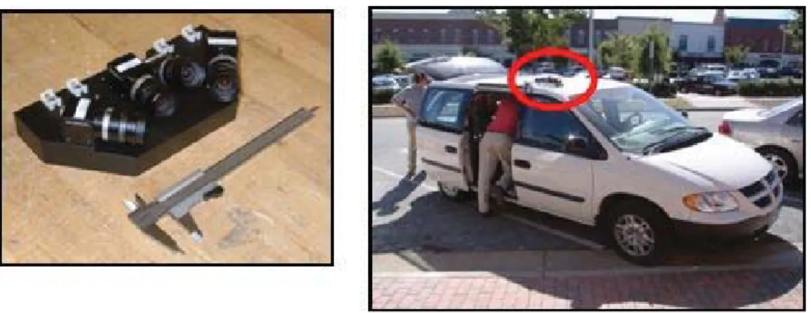
Figure 3.1: Example of a multi-camera system on a vehicle

with one point correspondence.

It can be difﬁcult to avoid losing part of the ﬁeld-of-view due of a single camera or omnidirectional camera due to occlusion, which may require camera cluster placement high up on a boom. Alternatively, for mounting on a vehicle the system can be split into two clusters so that one can be placed on each side of the vehicle and occlusion problems are minimized while giving a large baseline for scale estimation. In this chapter we will show that by using a system of two camera clusters, consisting of one or more cameras each, separated by a known transformation, the six degrees of freedom (DOF) of camera system motion, including scale, can be recovered.

An example of a multi-camera system for the capture of ground-based video is shown in Figure 3.1. It consists of two camera clusters, one on each side of a vehicle. The cameras are attached tightly to the vehicle and can be considered a rigid object. This system is used for the experimental evaluation of our approach.

(58)

(a) (b)

Figure 3.2: (a) Overlapping stereo camera pair, (b) Non-overlapping multi-camera system

extended periods of time by using a known baseline and cameras with overlapping ﬁelds of view. Our approach eliminates the requirement for overlapping ﬁelds of view and is able to maintain the absolute scale over time.

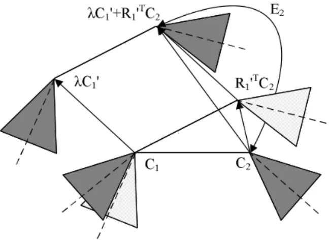
In the next section 3.2, we introduce our novel solution to ﬁnding the 6DOF motion of a two-camera system with non-overlapping views. We derive the mathematical basis for our technique in section 3.3 as well as give a geometrical interpretation of the scale constraint. The algorithm used to solve for the scaled motion is described in section 3.4. Section 3.5 discusses the evaluation of the technique on synthetic data and on real imagery.

3.2 6DOF Multi-camera Motion

The proposed approach addresses the 6DOF motion estimation of multi-camera systems with non-overlapping fields-of-view. Most previous approaches to 6DOF motion estima-tion have used camera configuraestima-tions with overlapping fields of view, which allow corre-spondences to be triangulated simultaneously across multiple views with a known, rigid baseline. Our approach uses a temporal baseline where points are only visible in one cam-era at a given time. The difference in the two approaches is illustrated in Figure 3.2.