STUDIES OF CHARGE ACCUMULATION IN THE KATRIN MAIN
SPECTROMETER
Kevin J. Wierman
A dissertation submitted to the faculty of the University of North Carolina at
Chapel Hill in partial fulfillment of the requirements for the degree of Doctor of
Philosophy in the Department of Physics and Astronomy.
Chapel Hill
2016
Approved by:
John WilkersonReyco Henning
Joaqu´ın Drut
Gerald Cecil
c
O2016
ABSTRACT
Kevin J. Wierman: Studies of Charge Accumulation In The KATRIN Main Spectrometer. (Under the direction of John Wilkerson.)
Experiments in recent years have shown neutrinos have non-zero rest mass. The Karlsruhe
Tritium Neutrino experiment (KATRIN) will directly probe the electron anti-neutrino mass using
tritium beta decay. KATRIN’s main spectrometer aims to provide a 0.2 eV sensitivity to the neutrino
mass, an order of magnitude improvement over the previous generation of experiments. During
KATRIN’s most recent commissioning phase, a mono-energetic electron source was used to probe
transmission properties and study associated potential systematic errors in the main spectrometer.
Charge accumulation from this source is identified as a potential source for systematic error and the
ACKNOWLEDGMENTS
Funding provided by the DOE Office of Science under grant numbers: #
TABLE OF CONTENTS
List of Figures . . . xi
List of Tables . . . xii
List of Abbreviations and Symbols . . . xiii
1 Neutrino Mass . . . 1
1.1 Current Description . . . 1
1.1.1 Dirac Description . . . 2
1.1.2 The Standard Model . . . 2
1.1.3 Oscillation Experiments . . . 3
1.1.4 Majorana Neutrinos . . . 5
1.2 Neutrino Mass Measurements . . . 6
1.2.1 Cosmological Measurements . . . 6
1.3 Neutrinoless Double Beta Decay . . . 7
1.4 Kinematic Neutrino Mass . . . 8
1.4.1 Tritium Beta Decay Measurements . . . 9
1.4.2 Other Direct Neutrino Mass Measurements . . . 12
1.5 Impact of Neutrino Mass Measurements . . . 13
2 Magnetic Adiabatic Collimation and Electrostatic Filtering . . . 15
2.1 Introduction . . . 15
2.2 Methodology . . . 15
2.3 Resolution . . . 17
2.4 Transmission Function . . . 18
2.5 Angular Acceptance . . . 19
2.6 Design . . . 20
2.8 Introducing a Dipole Field . . . 22
2.8.1 Regular Motion without the Dipole Electrode . . . 23
2.8.2 Motion With a Dipole Electrode . . . 26
2.8.3 Trap Emptying by Dipole Electrode . . . 28
2.9 Application . . . 29
3 KATRIN. . . 30
3.1 Experimental Goal . . . 30
3.2 Apparatus . . . 30
3.2.1 Windowless Gaseous Tritium Source . . . 31
3.2.2 Differential And Cryogenic Pumping Sections . . . 32
3.2.3 Spectrometers . . . 33
3.2.4 Detector . . . 35
3.2.5 Detector Wafer and Electronics . . . 37
3.2.6 Data Acquisition Electronics . . . 38
3.2.7 Cosmic Ray Veto . . . 41
4 Spectrometer and Detector Section Commissioning . . . 43
4.1 Goals . . . 43
4.2 Commissioning Apparatus . . . 44
4.2.1 The Electron Gun . . . 44
4.2.2 Method of Measuring Transmission Functions . . . 48
4.3 EGun Evaluation . . . 49
4.4 KATRIN Software . . . 50
4.4.1 Geometry . . . 50
4.4.2 KEMField . . . 52
4.4.3 Kassiopeia . . . 53
4.4.4 Preliminary Simulation Results . . . 54
4.5 EGun Simulation Applications . . . 54
5 Charge Accumulation. . . 56
5.1 Initial Indications of Charge Accumulation . . . 56
5.2.1 Dipole Electrode Effect . . . 62
5.2.2 Analytic Model Evaluation . . . 64
5.3 Measurement of Charge Accumulation . . . 69
5.3.1 Method . . . 69
5.3.2 Rate Acquisition . . . 70
5.3.3 Measured Transmission Function . . . 73
5.3.4 Residual Rate Calculation . . . 74
5.3.5 Fitting Rate Excess . . . 75
5.4 Simulation of Trapped Particles . . . 78
5.4.1 Simulation Construction . . . 79
5.4.2 Results of Simulations . . . 81
5.5 Comparison of Simulations and Analysis Results . . . 86
5.6 Dipole Electrode Model Analysis . . . 89
5.7 Null Hypothesis Testing . . . 90
5.8 Neutrino Mass Impact . . . 91
6 Conclusion . . . 94
6.1 Summary of Results . . . 94
6.1.1 Dipole Electrode Model . . . 94
6.1.2 Electron Gun Simulation . . . 94
6.1.3 Charge Accumulation Model . . . 95
6.1.4 Neutrino Mass Impact . . . 95
6.2 Moving Forward . . . 95
6.3 Outlook . . . 96
Appendix A Thorough Derivation of MAC-E filtering . . . 97
Appendix B Correlation Checking the Data against Slow Controls Values. . . 102
B.1 Correlation Searches . . . 102
B.1.1 Binning . . . 102
B.1.2 Correlation Strategies . . . 102
B.1.3 Correlation Testing . . . 103
B.1.5 Correlation Difference . . . 104
Appendix C The FPD Cosmic Ray Veto . . . 108
LIST OF FIGURES
1.1 Neutrino mass hierarchy . . . 5
1.2 Tritium beta decay spectrum . . . 9
1.3 Tritium final state modification energies . . . 11
1.4 Neutrino mass impact . . . 13
2.1 Design of a MAC-E filter . . . 17
2.2 Transmission function for an isotropic and monoenergetic source of electrons . . . . 19
2.3 A simplified Penning Trap . . . 21
2.4 Electron motion with dipole shift . . . 23
2.5 Simple cyclotron motion . . . 25
2.6 Cyclotron motion with magnetron drift . . . 27
3.1 The KATRIN apparatus . . . 31
3.2 The windowless gaseous tritium source . . . 32
3.3 The cryogenic and differential pumping systems . . . 33
3.4 The prespectrometer . . . 34
3.5 The KATRIN main spectrometer . . . 35
3.6 The KATRIN focal plane detector . . . 36
3.7 The assembled KATRIN detector system . . . 37
3.8 The effect of the KATRIN post acceleration electrode . . . 38
3.9 The KATRIN detector wafer . . . 39
3.10 The detector feedthrough flange . . . 39
3.11 The detector front-end electronics . . . 40
3.12 ORCA readout of the KATRIN detector . . . 41
3.13 FPD Signal through the Mark IV trapezoidal filter . . . 42
3.14 Example data collection at detector . . . 42
4.1 The SDS commissioning apparatus . . . 43
4.2 Schematic of the commissioning electron gun . . . 44
4.4 The interior of the electron gun . . . 46
4.5 The EGun photoelectric surface . . . 47
4.6 EGun high voltage schematic . . . 47
4.7 Example transmission function measurement . . . 49
4.8 Simulated main spectrometer . . . 50
4.9 Simulated EGun geometry . . . 51
4.10 EGun electrostatic potential map . . . 52
4.11 Particle tracks in the EGun . . . 53
4.12 Example simulated transmission function . . . 54
5.1 Hysteresis in the transmission function . . . 57
5.2 Simulated dipole geometry . . . 58
5.3 KATRIN commissioning potential map . . . 59
5.4 Maximum transmission angle as a function of initial energy . . . 60
5.5 Trapping probability as a function of position . . . 61
5.6 Analytic transmission function with charge accumulation . . . 65
5.7 Analytic transmission function excess . . . 66
5.8 Mean rate impact on electron rate excess fits . . . 67
5.9 Energy distribution impact on excess fits . . . 68
5.10 Region of interest adjustment . . . 72
5.11 Region of interest adjustment . . . 73
5.12 Measured transmission function . . . 74
5.13 Dipole measurement residuals . . . 75
5.14 Individual Measured Transmission Function Residuals . . . 76
5.15 Dipole measurement residual fits . . . 77
5.16 Initial Distributions of electrons in simulation . . . 79
5.17 Simulated number of trapped electrons . . . 81
5.18 Simulated dipole effect on transmission function . . . 82
5.19 Simulated transmission function with charge accumulation . . . 83
5.21 Individual Simulated Transmission Function Residuals . . . 85
5.22 EGun width broadening from dipole electrode . . . 87
5.23 Event Lifetime as a function of dipole potential . . . 88
5.24 Number of turns spent in the main spectrometer . . . 89
5.25 Dipole reduction constant comparison . . . 91
5.26 Neutrino mass impact . . . 93
C.1 Schematic drawing of the KATRIN veto . . . 108
C.2 The St. Gobain fibers used to read out the scintillator panels. . . 108
C.3 MPPCs . . . 109
C.4 Veto panels . . . 110
C.5 Fiber end closeup . . . 111
C.6 Veto biasing electronics . . . 112
C.7 New veto enclosure design . . . 112
C.8 Assembled veto panels . . . 113
C.9 MPPC sample output . . . 114
C.10 Digitized veto signal . . . 115
C.11 Veto digitization comparison . . . 116
C.12 FPGA triggering rates for veto . . . 117
C.13 Veto peak peak finding . . . 118
C.14 Veto spectral stability . . . 119
C.15 Veto hodoscope measurement . . . 120
LIST OF TABLES
1.1 Results of oscillation experiments . . . 4
1.2 Neutrino mass results from cosmology . . . 6
1.3 Neutrino mass results from neutrinoless double beta decay. . . 8
1.4 Limits on neutrino mass from Tritium Beta Decay Experiments . . . 10
4.1 Nominal Electrode Potentials . . . 49
4.2 Measured EGun Properties . . . 50
5.1 Run Numbers . . . 70
5.2 Backplate Voltages Used in Study . . . 71
5.3 Fit results for measured data . . . 78
5.4 Fit results for simulated data . . . 86
5.5 Dipole Effect on Transmission Width . . . 87
6.1 Summary of KATRIN Systematics . . . 96
B.1 Linear Correlation With Slow Controls parameters . . . 105
B.2 Correlation Residuals . . . 105
B.3 Correlation coefficients for background runs . . . 106
LIST OF ABBREVIATIONS AND SYMBOLS
νe, νµ, ντ Neutrino Flavor Eigenstates
ν1, ν2, ν3 Neutrino Mass Eigenstates
m1, m2, m3 Neutrino Mass Eigenvalues
mβ Kinematic Neutrino Mass
mββ Effective Majorana Mass
mcosm Cosmological Neutrino Mass
T Transmission Ratio
U0 Analyzing Potential
Ee Electron Energy
θpch Pitch Angle
BS Source Magnetic Field
BA Analyzing Magnetic Field
Bmin Minimum Magnetic Field
Bmax Maximum Magnetic Field
KATRIN Karlsruhe Tritium Neutrino Mass Experiment
MAC-E Magnetic Adiabatic Collimation and Electrostatic filtering
WGTS Windowless Gaseous Tritium Source
DPS Differential Pumping System
CPS Cryogenic Pumping System
FPD Focal Plane Detector
SDS Spectrometer and Detector Systems
EGun Electron Gun
TF Transmission Function
ROI Region of Interest
HV High Voltage
CHAPTER 1: NEUTRINO MASS
The goal of this dissertation is to aid the measurement of the mass of the electron anti-neutrino.
This chapter discusses the physics of neutrino mass and absolute mass measurements.
1.1 Current Description
One of the most abundant particles in the universe, the neutrino, is the focus of a field of study
with broad impacts across physics. In cosmology, neutrinos parameterize mass density in the epoch
immediately following the Big Bang. Astrophysics utilizes neutrinos to describe nuclear reactions in
solar models and observations of supernovae neutrinos are used in nuclear astrophysics to describe
core collapse. Nuclear and particle physics experimentally probes the origins of mass with neutrino
observations to improve the Standard Model of particle physics. However, several properties of
neutrinos described in this chapter have not yet been measured and their measurement will provide
insights to the fields impacted by neutrinos.
The existence of neutrinos was postulated due to the continuity of the beta decay energy
spec-trum and the associated spin statistics [1]. In beta decay, a continuous electron energy spectra
implies that a third particle must participate in the interaction [2]. Equation 1.1.1, represents the
decay from a parent nucleus,AZX to the child nucleus, A
Z+1X, and an electron, e −
, and this third
body,νe, theelectron anti-neutrino.
A ZX →
A
Z+1X+e −
+νe (1.1.1)
From the process in Equation 1.1.1, one can infer that to conserve angular momentum and
electronic charge, neutrinos must be charge neutral fermions. In addition, similar to other charged
fermions, neutrinos come in three interaction flavors. In this case, these are electron neutrinos (νe),
muon neutrinos (νµ), and tau neutrinos (ντ) [3–5]. We now know that this process (and the inverse
process) are explained by the weak interaction [6, 7]. Currently this interaction is the only known
process by which neutrinos are created or consumed. The eigenstates for this process correspond to
1.1.1 Dirac Description
In the Dirac description of particle physics, fermions are described by four components; particle
and anti-particle states and two spin projections. These four component spinors obey the Dirac
equation in Equation 1.1.2. In this equation, the particle wavefunction, ψ is operated on by the
4-gradient,∂/, which mixes spin projections, and the scalar mass term,m, which does not mix spin
projections. A particle whose wavefunction obeys the Dirac equation must then have both spin
projections or be massless. Therefore, if neutrinos are massive and if neutrinos are described by the
Dirac equation, then neutrinos must exist in both spin projections orhelicities.
(i /∂−m)ψ= 0 (1.1.2)
However, neutrinos are observed to be produced only in a single helicity. Polarized beta decay
experiments have shown that electrons produced in beta decay can only be produced with spin in the
same direction as their momenta, or positive helicity [8, 9]. Due to angular momentum conservation,
neutrinos are then only produced with negative helicity, and anti-neutrinos with positive helicity.
This also shows that weak interactions are parity violating.
1.1.2 The Standard Model
The standard model of particle physics describes fundamental interactions as gauge bosons
and the participating particles as fermionic fields[7]. As weak interactions are parity violating, an
alternative description known as chirality is used to describe particle field operators. Here, the
chirality of a particle is analogous to the helicity and in fact is identical for massless particles. Like
with helicity, neutrinos only appear in chirality with left-handed particle states and right-handed
anti-particle states.
In the standard model, particles are initially required to be massless to guarantee gauge
invari-ance. The Higgs mechanism necessitates additional terms in the Lagrangian which include particle
mass [7]. In this mechanism, fermion masses show up as the vacuum expectation value, v of the
Higgs doublet, φ0. This doublet is included in the Yukawa coupling terms of the standard model
Lagrangian. For the case of neutrinos, the Yukawa term of the Lagrangian density for electrons
is shown in Equation 1.1.3 where the Higgs doublet couples to the left handed fermion doublet,
Lyuk=−ce ¯
eRφ
† 0 νeL eL
+ (¯νeL,e¯L)φ0eR
(1.1.3)
φ0=√1
2 0 v (1.1.4)
From this description, the mass of electrons is generated. However, for neutrinos, mass is
required to be zero due to the right handed singlet terms having no neutrino term with which to
couple. This is a result of requiring both handed-states to couple to the Higgs doublet, but as only
one handed-ness is observed, the mass term is zero.
1.1.3 Oscillation Experiments
Neutrinos have been shown to have non-zero masses due to the phenomena known asneutrino
oscillations. Suppose that the neutrino flavors from Section 1.1.1 are not singularly associated to
their mass eigenstates, ν1, ν2, ν3 with eigenvalues m1, m2, m3. Instead, a rotation, Uα,i forms a
general relation between the flavor and mass states as shown in Equation 1.1.5.
να=X
i
Uα,iνi (1.1.5)
This formalism can be inserted into the propagator for particles in vacuum to calculate the
probability of detecting a neutrino in state να that was originally produced in state νβ. This is
detailed in Equation 1.1.6 where t is time, δαβ is the Dirac delta, L is length from source, and E
is the initial energy of the particles. The mass squared difference, ∆m2ij is the difference in mass
eigenvalues,miandmjsquared. Thus, a non-zero mass squared difference and off-diagonal elements
in the mixing matrix require at least one massive eigenstate.
P(να→νβ) =
hνβ|να(t)i
2 =
δαβ+ X
i6=j
Uβie
−i∆m 2
ij L
2E U∗ αj 2 (1.1.6)
Experimentally, the mixing matrix is probed by observing the flux of neutrinos from solar sources,
atmospheric sources, reactors and accelerators. At different energies and length scales, this allows
sensitive to energies where ∆m2ijL/2E ≈ ±1, and so it is useful to utilize subscripts which indicate
the source of the neutrinos instead of the mass eigenstate indices.
In Equation 1.1.7, the parameters, δ, α1, and α2 parameterize the probability of CP phase
violation. This occurs when the probability of a particle oscillating into a flavor is not identical to
the anti-particle case. This violates the symmetry of the C and P operators. The charge conjugate
operator, C transforms a particle state into an anti-particle state and the parity operator P performs
a spatial inversion of one ordinate. For the case of the terms denoted,Majorana in Equation 1.1.7,
these require that neutrinos are their own antiparticle and will be discussed in Section 1.1.4.
The current results of oscillation experiments are detailed in Table 1.1.3. Current efforts are
being made to improve measurements of these results [10–12]. Since the mass difference squared
values are observed to be non-zero, one deduces that neutrinos are massive. In addition, by setting
the lightest mass eigenstate to zero, one may set a lower limit on the neutrino masses using the mass
squared differences. U =
1 0 0
0 c23 s23
0 −s23 c23
(Solar)
c13 0 s13e−iδ
0 1 0
−s13e
iδ
0 c13
(Reactor)
c12 s12 0
−s12 c12 0
0 0 1
(Atmospheric)
eiα1 0 0
0 eiα2 0
0 0 1
(M ajorana) (1.1.7)
Parameter best fit(±1σ) 3σ
∆m2solar[10
−5
eV2] 7.58−+00..2226 6.99−8.18 ∆m2atm[10
−3
eV2] 2.35−+00..1209 2.06−2.67 sin2θ12 0.306(0.312)
+0.018
−0.015 0.259(0.265)−0.359(0.364) sin2θ23 0.42
+0.08
−0.03 0.34−0.64
sin2θ13 0.021(0.025) +0.007
−0.008 0.001(0.015)−0.044(0.036)
Table 1.1: Results of oscillation experiments. These recent findings were summarized by the Particle Data Group in Table 14.7 [13].
While these experiments show neutrino mass exists, the mass term in Equation 1.1.6 is only
sensitive to mass squared differences. The sign of the difference can be found by using matter
effects [14]. Currently, this is done for atmospheric neutrinos and solar neutrino measurements are
underway. This allows for two possible mass eigenstate orderings or hierarchies, as illustrated in
Figure 1.1: The possible hierarchies of neutrino masses and the associated flavor mixing in each flavor eigenstate. Image sourced from: [15].
Massive neutrinos show that the description used in the standard model is either incomplete or
incorrect.
1.1.4 Majorana Neutrinos
An alternative to the Dirac description of particles is the Majorana description [16]. In
compar-ison to the Dirac equation, the Majorana equation as shown in Equation 1.1.8 shows no distinction
between particles and anti-particles and their associated helicities. Instead, this equation now mixes
the particle states with their charge conjugates,ψc.
i /∂ψc+mψ= 0 (1.1.8)
As neutrinos are charge neutral, they are candidates for being used in the Majorana equation [16].
In this description, neutrinos and anti-neutrinos would be the same particle with different
handed-ness. The Majorana equation therefore provides an alternative description for neutrinos, which may
be used to amend the standard model to account for neutrino mass. However, this requires that
1.2 Neutrino Mass Measurements
In addition to neutrino oscillation experiments, several different techniques can be used to probe
neutrino mass. These include cosmological measurements, neutrinoless double beta decay and single
beta decay kinematics measurements. The measurements provide complimentary information on
neutrino mass and the other remaining unmeasured neutrino parameters.
1.2.1 Cosmological Measurements
In analogy to the standard model of subatomic physics, ΛCDM, or dark energy, the λ model
with cold dark matter, CDM, is the analytical model against which to compare cosmological
obser-vations [17]. This model describes the evolution of the universe starting from a hot dense state to
today’s universe. Observables in this model include large scale structures and anisotropies in the
cosmic microwave background[18].
The ΛCDM model predicts a relic neutrino background distributed throughout the universe.
These neutrinos originate from electroweak freeze out just after the big bang, and therefore their
expected energy should be in the region of the Q-value for neutron decay, namely in the sub-meV
region. While this low threshold makes relic neutrinos difficult to impossible to detect, the connection
between neutrinos and ΛCDM makes neutrino mass a parameter in the model. The energy density
of neutrinos, Ων can be compared to the energy density of the universe as a whole, Ωtotand can be
computed as
Ων= P
imi
93.14h3eV /c2 (1.2.1)
Where h is the dimensionless Hubble parameter[19].
For comparison, a 2 eV neutrino mass here results in a fractional energy density comparable to
that of baryonic matter. Measuring this parameter is achieved by fitting a number of parameters to
cosmological data sets. Recently the Planck collaboration has released an analysis which is shown
in Table 1.2.
Upper Limit Confidence Limit
mi<0.230eV /c
2
95%
Table 1.2: Neutrino mass results from cosmology. Result sources from: [18].
This limit was achieved by combing data sets from Planck with data sets from the Wilkinson
by fitting the data to the ΛCDM model, this represents a model dependent measurement. In
addition, multiple correlated fit parameters are used in the fits. Therefore, if a separate neutrino
mass measurement is performed, then these models can be constrained by neutrino mass rather than
utilizing it as a fit parameter.
1.3 Neutrinoless Double Beta Decay
Observations of neutrinoless double beta decay can provide another means of obtaining a
neu-trino mass measurement. Two neuneu-trino double beta decay is a rare process in which two beta decays
simultaneously occur, and is found in nuclei where normal beta decay is energetically forbidden[20].
This process is characterized in Equation 1.3.1 where the nucleus decays to the daughter nucleus
plus two electrons and neutrinos.
A ZX→
A
Z+2X+ 2e −+ 2ν
e (1.3.1)
If neutrinos can be described by the Majorana equation in Section1.1.4, then it is possible that
instead of emitting two neutrinos, none are emitted as in Equation 1.3.2. While multiple processes
can explain the internal mechanism for this decay, the simplest model involves the exchange of a
virtual Majorana neutrino between nucleons [21]. Since the weak interaction requires emission in
one helicity and absorption in another, the spin of the virtual neutrino must flip.
A ZX →
A
Z+2X+ 2e −
(1.3.2)
Neutrino mass in neutrinoless double beta decay is related to the probability of this change of
helicity. The half life of this process is effected by the virtual Majorana neutrino exchange. This
is related to an effective “Majorana mass” of neutrinos, hmββi in Equation 1.3.3. The mass term,
hmββi
2
is expressed in terms of fundamental quantities in Equation 1.3.4. This also depends on
the phase factor for two electrons, G0ν, the weak coupling constant, gA and the transition matrix
element,M(0ν).
T10/ν2
−1
=G0νg
4
A
M
(0ν) 2
hmββi
2
(1.3.3)
hmββi2= X i
Uei2mi
Currently, several experiments are utilizing neutrinoless double beta decay for neutrino mass.
Notably among these, EXO-200 [22], Gerda [23], Kamland-Zen [24] have set upper limits on the
effective Majorana mass detailed in Table 1.3. This limit is valid only if neutrinos can be described
by the Majorana equation. If neutrinos are Dirac particles, then no such sensitivity can be obtained.
Therefore, the measurement of the effective Majorana mass is dependent on the Majorana neutrino
model.
Upper Limit Confidence Limit
hmββi<0.2−0.4eV /c
2
95%
Table 1.3: Neutrino mass results from neutrinoless double beta decay.
Measuring the neutrino mass in this method provides additional information on the Majorana
vs Dirac nature of the neutrino. However, this method is limited by uncertainties in the weak
coupling constant and the choice of nucleus and therefore nuclear matrix element[25]. This can be
complimented by a direct measurement of the neutrino mass which has no dependency on these
values.
1.4 Kinematic Neutrino Mass
Of the methods for measuring neutrino mass, using the kinematics of beta decay is the most
direct and is model independent. Following the Fermi theory of beta decay, the rate of electrons
produced with energyE and momentumpis given by Equation 1.4.1 [26].
dN
dE =C|M|
2
F(Z, E)p(E+me)(Q0−E) X
j
Uej q
(Q0−E) 2
−m2jΘ(Q0−E−mβ) (1.4.1)
C=G 2
Fm
5
e
2π3 cos
2
(θC) (1.4.2)
X
j
Uje
q
(Q0−E)2−m2j ≈ q
(Q0−E)2−m2β (1.4.3)
m2β= X
i |Uje|
2
|mj|
2
(1.4.4)
Here, the endpoint energy, Q0 is the maximum electron energy corresponding to a massless
neutrino model. The Heaviside step function, Θ, ensures conservation of energy. The leading
coefficient,C containsGF, the Fermi constant,θC, the Cabibbo angle, andme, the electron mass.
Nuclear wavefunction overlap is included in the nuclear matrix element, M. The Fermi function
Equations 1.4.3 and 1.4.4 show an approximation commonly used in the context of neutrino mass.
Currently, the experimental sensitivity to term is insufficient to determine the mass eigenstates,mj.
Therefore, the sum over the PMNS matrix terms are absorbed into the square root to form the term,
mβ, sometimes referred to as the kinematic neutrino mass.
As none of these values in Equation 1.4.1 are model dependent and this observation relies on no
assumptions regarding neutrinos, this is a direct method to determine neutrino mass. Commonly
this is referred to asabsolute neutrino mass.
Neutrino mass is measured by fitting the shape of the observed electron energy spectrum to
Equation 1.4.1. The energy spectrum is most sensitive to neutrino mass in the region whereE ≈
Q0−mβ. It is therefore desirable to utilize a beta emitter with a low Q-value. The common
experimental method is to then observe the electron energy spectrum coming from beta decay and
fit the endpoint region spectral shape to the neutrino mass in Equation 1.4.4.
1.4.1 Tritium Beta Decay Measurements
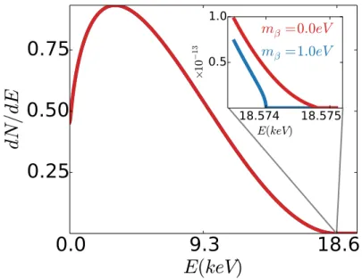
Figure 1.2: Tritium beta decay spectral shape for atomic tritium without final state effects. The embedded plot is the spectrum near the endpoint region. The red and blue lines show the spectral shape with a 0.0 eV and a 1.0 eV neutrino mass, respectively.
Tritium is a commonly used source in kinematic neutrino mass measurements. This is due to
tritium’s low endpoint energy (18.6 keV), super-allowed decay, simple nuclear properties and simple
atomic structure. Equation 1.4.5 shows the decay process for tritium. Currently, the best limits on
T →3He+e−+ ¯νe+Q0 (1.4.5)
Using the current best limits on neutrino mass to set the region of interest, the number of
electrons in the 2 eV range below the endpoint account for 1 in 1013electrons emitted in beta decay.
Figure 1.2 shows the expected spectral shape for this case. The inset figure shows the portion of the
spectrum with sensitivity to a 1eV neutrino mass, and thus illustrates the need to utilize as many
electrons as possible without modifying the spectral shape. A high precision experiment therefore
needs good resolution in this region, low backgrounds and high acceptance for electrons produced
by a highly luminous source.
Experiment Result C.L.
Mainz[28] 2.3 eV 95% Troitsk[27] 2.2 eV 95%
Table 1.4: Limits on neutrino mass from Tritium Beta Decay Experiments
The next generation of neutrino mass experiments will need to incorporate the previously
men-tioned requirements if the sensitivity to neutrino mass is to be increased. In addition, potential
systematic errors which effect a lower neutrino mass sensitivity must be addressed.
Final States in Tritium Beta Decay
A potential systematic error in the neutrino mass measurement arises in the energy lost due to
atomic and molecular final states of the decay source.
Using molecular tritium as a decay source is the most sensitive technique to probe the neutrino
mass via the beta decay spectrum. This is due to the well understood and minimal systematic errors
from scattering in the source itself [26]. One modification of the spectrum that must be accounted
for is associated with the excitations formed in the daughter molecule of the decay.
Molecular tritium,T2decays according to Equation 1.4.6, where the daughter molecule, 3
HeT+,
can be an excited state. Excitations arise from rotational and vibrational modes of the bound
molecular state and electronic excitations in the molecular ion [30, 31].
T2→ 3
HeT++e−+νe+Q0 (1.4.6)
The tritium spectrum endpoint region is modified by the energy lost to excitations.
0
50
100
150
200
250
E
i[
eV
]
10
-710
-610
-510
-410
-310
-210
-1ω
iFigure 1.3: Tritium final state energy distribution. The x axis shows the energy lost in each final state branch which occurs with probabilitywi. Data sourced from [29].
In contrast to the unmodified spectrum in Equation 1.4.1, each branching ratio modifies the spectral
shape similar to produce a systematic error if left unaccounted for.
dN
dE =C|M|
2
F(Z, E)p(E+me) X
i,j
wi(Q0−Ei−E)Uej q
(Q0−Ei−E)
2
−m2jΘ(Q0−Ei−E−mβ)
(1.4.7)
These effects are currently being measured to a higher precision by the TRIMS experiment at
the University of Washington [32]. Figure 1.3 shows the distribution of energies which are clearly
dominated by the electronic states in the region>10eV. Not shown in this plot are the nuclear final
state distributions that are from impurities in the source. Naturally occurring tritiated hydrogen
isotopologues, DT andHT have reduced masses and therefore different excitation spectra. Before
the next generation of tritium neutrino mass experiments move forward, each of these spectra will
be quantitatively analyzed by the TRIMS experiment.
The neutrino mass sensitivity can be limited by the systematic uncertainty quantified by these
measurements. For instance, a 1% uncertainty in the width of the distribution of molecular final
states would correspond to a standard deviation on the order of 10−3eV2 in the measurement of
the square of the neutrino mass. Therefore, moving forward requires knowledge of the final state
1.4.2 Other Direct Neutrino Mass Measurements
In addition to the neutrino mass measurement that is the focus of this thesis, several other
measurements aim to make a directly probe the kinematic neutrino mass.
Project 8
Cyclotron radiation emission spectroscopy is the method of measuring the power of the
radi-ation produced by electrons undergoing cyclotron motion in strong magnetic fields. The Project
8 collaboration[33] is utilizing this concept to obtain a neutrino mass measurement from tritium
placed in high magnetic fields. The cyclotron radiation emitted by these electrons is described in
Equation 1.4.8 where the frequency, ω is a related to the kinetic energy, Ee through the Lorentz
factor,γ.
ω= eB
γme
= ωc
1 +Ee/(mec
2
) (1.4.8)
Measuring the cyclotron frequency is a non-destructive measurement and therefore allows the
electrons to be used with other detectors for gating purposes. At a 1 T magnetic field, the Q-value
of the tritium spectrum produces a 26 GHz signal. Radiofrequency waveguides placed around the
volume pick up the radiation whose power is modified by the Larmor formula in Equation 1.4.9.
P(β, θ)∝ 2
3
q2ωc2p2⊥ m2ec
3 (1.4.9)
Higher power signals are favorable due to increasing the signal to noise ratio. By design, those
with high pitch angle provide a higher measurement time and will be easiest to detect.
Project 8 presents another measurement of the neutrino mass which can be used to test
KA-TRIN’s findings. Multiple measurements are favorable in order to compare systematic uncertainties.
Electron Capture
Currently the other popular measurement method in direct neutrino mass determination is
electron capture on 163Ho. The kinematics of electron capture are nearly identical to that of beta
decay with the notable exception that the energy is modified by excitations in the daughter nucleus.
This is shown in Equation 1.4.10 where the excitations are modeled as Bright-Wigner peaks at
dN
dE =C|M|
2
F(Z, E)p(E+me)(Q0−E) q
(Q0−E) 2
−m2β X
i
Ci
Γi
2π((E−Ei) + Γ2i/4) (1.4.10)
This calculation is made in the sudden approximation of the overlap of the two electron wave
functions of holmium and the captured electron and multi-hole dysprosium excitation states.
Cur-rently, excitations with up to 3 electron holes have been calculated using the Dirac-Hartree-Fock
method. However, higher order calculations have been shown to be necessary for neutrino mass
determination. In addition, the measurements of the Q-Value of this process do not agree well.
Future measurements will need to reconcile these differences.
1.5 Impact of Neutrino Mass Measurements
1 − 10 1 3 − 10 2 − 10 1 − 10 1 3 −
103 10−2 10−1 1
− 10 2 − 10 1 − 10 1 1 − 10 1 3 − 10 2 − 10 1 − 10 1
[eV]
Σ
m
β[eV]
[eV]
βm
[eV]
ββm
(NH)
σ
2
(IH)
σ
2
1 −10 1 10−3 10−2 10−1 1
3 − 10 2 − 10 1 − 10 1 3 − 10 2 − 10 1 − 10 1
Figure 1.4: Possible neutrino mass solutions [36]. The exclusion regions are given by bounds from global fits using cosmological and oscillations data. The blue and red zones are dependent on the normal and inverted hierarchy respectively.
Given the information presented in previous sections, the unknowns in neutrino physics can be
What is the absolute scale of neutrino mass?
Are neutrinos their own antiparticle?
Why are neutrino masses much smaller than the mass of other fundamental particles?
Which possible ordering applies itself to neutrino mass?
Absolute neutrino mass is related to the other unknowns in physics. Figure 1.4 shows the
impact of each of the mass terms detailed above for both of the mass hierarchies allowed by neutrino
oscillation experiments. For instance, one may rule out the inverted hierarchy if the absolute neutrino
mass is low enough. The other open questions can be addressed similarly.
Whether or not neutrinos are their own anti-particle is determined by the observation of a
neutrinoless double beta decay mode as shown in Section 1.1.4. Figure 1.4 shows that if neutrinos
fall into the inverted hierarchy and kinematic neutrino mass is measured below the allowed range and
neutrinoless double beta decay is not observed below the allowed range for the inverted hierarchy,
then one may rule out the possibility of Majorana neutrinos.
This dissertation is focused on kinematic neutrino mass through tritium beta decay. The
fol-lowing chapter will discus the most sensitive experimental method for beta decay searches and the
CHAPTER 2: MAGNETIC ADIABATIC COLLIMATION AND ELECTROSTATIC FILTERING
This chapter discusses a spectrometer technology known as magnetic adiabatic collimation and
electrostatic filtering. This technology is used in the measurement of the tritium spectrum endpoint
region. The experimental focus of this thesis involves the usage of this method and particle trapping
effects inherent to the apparatus.
2.1 Introduction
As discussed in Section 1.4.1, measuring the neutrino mass to sub-eV sensitivity requires
ob-taining the energy spectrum from tritium beta decay to high precision in the endpoint region. This
level of precision requires:
Low background in the endpoint region
High angular acceptance from source
A highly luminous source
High resolving power in the endpoint region
These requirements are addressed by a technology known as magnetic adiabatic collimation and
electrostatic (MAC-E) filtering. This was the technique used by the Mainz and Troitsk experiments
to set the best direct limits on the electron anti-neutrino mass. While MAC-E filters were not
originally created for the purpose of analyzing tritium beta decay[37], MAC-E filters have historically
featured high acceptance and luminosity with high resolution [38].
2.2 Methodology
The basic framework of MAC-E filters is a series of superconducting solenoidial magnets
produc-ing magnetic field lines that connect the source to a detector. Electrons in a magnetic field undergo
cyclotron motion due to the Lorentz force with a guiding center along the magnetic field line. In a
cylindrically symmetrical system, up to half of the electrons produced in beta decay transmit toward
With a magnetic field guiding electrons from source to detector, spectroscopy is performed by
introducing an electrostatic potential normal to the magnetic field lines. The goal of using the
electrostatic potential is to precisely reflect electrons below a set potential,U0. From an isotropic
source such as tritium, electrons are created with a range of pitch angles,θpchbetween their momenta
and the magnetic field. The symmetry of the system allows the energy to be expressed as a sum
of the perpendicular and longitudinal energies as follows, for an electron produced with energy, Ee
and mass,m.
Ek= (p∗sin(θpch)) 2
2m (2.2.1)
E⊥ =
(p∗cos(θpch))
2
2m (2.2.2)
Ee=Ek+E⊥ (2.2.3)
Therefore, the electrostatic potential will reflect electrons with energy withEk < U0. As
elec-trons with different pitch angles but identical longitudinal energy have different total energy, the
spectrometer will filter electrons of different energies equally. Since the purpose of the spectrometer
is filter electrons based on total energy, the filter width of the spectrometer is defined by this
qual-ity. Therefore, precision of the spectrometer is limited by the range of θpch electrons are allowed
to take for a given total energy and allowed to transmit. Measuring the neutrino mass requires
high acceptance and therefore collimation is not a viable option to differentiate between electrons
of different pitch angles. However, re-aligning the electron momenta to the axis of symmetry would
be a preferable method to increase sensitivity.
In order to collimate electrons from the source, the magnetic field is slowly relaxed from the
maximum, Bmax to a minimum, Bmin where the electric potential is at it’s maximum, as shown
in Figure 2.2. In order to ensure adiabatic transfer and therefore minimize the loss in precision,
the first adiabatic invariant in Equation 2.2.4 must be conserved along the electron trajectory. In
this equation, γ is the relativistic Lorentz factor, andµ is the magnetic moment of the electron’s
cyclotron motion.
γµ= γ+ 1 2
E⊥
B =
γ+ 1 2
Ee−Ek
B (2.2.4)
A reduction in the magnetic field strength,B induces minimization of the perpendicular
Figure 2.1: Design of the MAC-E apparatus and momentum transformation. Image sourced from [39].
relaxation of the magnetic field realigns the momentum to the axis of symmetry. With the
electro-static potential,U0, applied at this magnetostatic minimum, the precision of the filter is increased.
The plane of symmetry for the electrostatic field is known as theanalyzing plane and is defined as
the plane where electrons with energyEk=U0 reflect.
2.3 Resolution
In general the momentum of an electron will not completely align with the beamline axis during
collimation. To show how this is possible, consider two cases. In the first case, an electron is
produced maximally aligned to the beamline, E⊥ = 0 with longitudinal energy Ek = Ee. At the
analyzing plane, this electron still hasEk =Ee. For the second case, an electron is produced with
longitudinal energy,Ek= (1−Bmax
Bmin)Ee. Then, at the analyzing plane, the electron has longitudinal
energy Ek = Ee. For both cases, the electrons are filtered by an electrostatic potential, U0 for
energiesEe < U0, and therefore to the spectrometer are identical. The latter case corresponds to
an electron with sin(θpch) = p
Bmin/Bmax, the maximum angle for transmitting electrons. The
adiabatic invariant for these two cases produces Equation 2.3.1.
Ee
Bmax
= ∆E
Bmin
Where Bmax and Bmin correspond to the maximum and minimum magnetic field strengths
respectively. The energy difference, ∆E is the difference in total energy between the maximally
aligned case and minimally aligned case. One can then express the resolution in terms of the
magnetic fields as in Equation 2.3.2.
∆E
E =
Bmin
Bmax
(2.3.2)
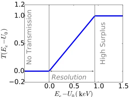
2.4 Transmission Function
While electrons with energy higher than the analyzing potential plus the resolution of the
spec-trometer will always transmit, and electrons below the analyzing potential always reflect, the
situ-ation where an electron is produced with energy within the resolution of the spectrometer is more
complex. The description of the ratio of the number of electrons transmitting to the number of
electrons produced at a given energy is referred to as thetransmission function orT(E).
Following the definition in Stefan Groh’s thesis[40], the transmission function for an initial
probability density function of electrons f(θpch, Ee) is computed as an integral over the allowed
angles and energies. Equation 2.4.1 shows a simplified version of the transmission function which
neglects relativistic effects for simplicity.. This is valid due to low Lorentz invariant in the Tritium
decay region.
T(E, U0) =
Z ∞
U0
Z θmax
0
f(θpch, Ee)dθpchdEe (2.4.1)
θmax=arcsin
s
(Ee−qU0)/EeBmin Bmax
!
(2.4.2)
The integral over the pitch angle is performed first due to the maximum allowed angular
de-pendence on the initial energy of electrons. The maximum angle, θmax is a function of the initial
electron energy and relative field strengths.
For the simple case of a source distributed isotropically in the maximum magnetic field with
Gaussian distributed energies, the resulting transmission function is shown in Equation 2.4.3.
Ap-pendix A shows the full calculation used to produce this. Graphically, this is displayed in Figure 2.2
where the transmission function has been shifted relative to the analyzing potential,U0. The x-axis
k
Figure 2.2: Transmission function for an isotropic and monoenergetic source of electrons
T(E) =
0 E≤qU0
1−q1−E−qU E
Bmin
Bmax qU0≤E≤qU0 Bmin Bmax
1 qU0
Bmin Bmax ≤E
(2.4.3)
The transmission function is an observable that can be used to obtain the resolution of a
spec-trometer experimentally. For a monoenergetic source with isotropic angular distribution, the
res-olution as shown in Figure 2.2 is the width of the transmission function. More complex electron
sources may also be used to probe the transmission function if the source spectral shape is known.
The basic workflow of using a MAC-E spectrometer is therefore to count the number of electron
transmitting from a tritium source for a number of analyzing potentials. This measures an integrated
spectrum where each point is the integral of the spectrum in Equation 1.4.5 fromU0to the Q-value
of the decay convolved with the transmission function.
2.5 Angular Acceptance
In general, the source of electrons is not required to be in the highest magnetic field strength.
Due to technical limitations, the maximum field strength is determined by the design of the
ideally one would increase the radius at the source and the corresponding magnetic flux. However,
the increase in magnetic field strength from source to magnet results in the magnetic reflection of
electrons with high pitch angle.
Angular acceptance in MAC-E filters is determined by magnetic reflection. Rearranging
Equa-tion 2.2.4 in terms of the source magnetic field,Bsrc results in Equation 2.5.1. The critical angle,
θc defines the maximum pitch angle with which electrons can be produced and not be magnetically
reflected. Therefore, angular acceptance is defined byθpch < θc for all azimuthal angles.
Bsrc Bmax
=sin2θc (2.5.1)
2.6 Design
Neutrino mass sensitivity in MAC-E filters is related through Monte Carlo simulation[41] to
luminosity, background rate, measurement time and spectrometer resolution. Of these parameters,
resolution is immutable to the apparatus.
As resolution increases with the ratio of field strengths, either the maximum field needs to be
increased or the minimum decreased. Increasing the maximum field strength is problematic because
technological limitations force the bore of the magnets to be smaller, decreasing luminosity[42].
Therefore, the minimum field strength must be decreased.
Since the adiabatic requirement must be met, the invariant in Equation 2.2.4 can be used to
calculate the size of the spectrometer. The adiabatic invariant is linearly related to the magnetic flux
through the helical orbit of electrons in cyclotron motion in Equation A.0.4. Therefore, to increase
the resolution of a MAC-E spectrometer and therefore it’s sensitivity to neutrino mass the radius of
the spectrometer must also be increased.
2.7 Charge Trapping in MAC-E Experiments
In previous experiments utilizing MAC-E filter technology, a common issue has arisen with
particles trapped in magnetic bottles and electrostatic minima [43–50]. Commonly, these areas of
charge accumulation are referred to as Penning Traps[41, 51] (or Penning-Malmberg traps depending
on the geometry), and a simplified drawing of one is given in Figure 2.7, whereby a strong magnetic
field confines a particle radially and the electrostatic quadrupole confines the particle axially.
In MAC-E filters, Penning traps occur due to electrostatic and magnetostatic confinement. The
Figure 2.3: A simplified Penning Trap. The red boxes indicate the solonoid inducing the magnetic field. Blue electrodes are configured in an electrostatic quadropole. The particle depicted in the center experiences a confining axial electrostatic force and a radially confining cyclotron motion. Image sourced from: [52].
to the analyzing potential by a magnetic field line. If the electron produced at the source does
not meet the requirement for transmission, then the electron is confined by the analyzing potential
and the source potential. Therefore, the probability of trapping for charged sources is the same as
reflection or,
Ptrap(E) = 1−T(E) (2.7.1)
WhereT(E) is the transmission function for source at energy,E.
The consequences of Penning traps in these spectrometers are twofold.
1. Electrons exiting the trap may create unwanted background
2. If the field sourced by trapped electrons becomes competitive with the analyzing potential,
then the electrons see a flat potential and all exit at once.
Penning traps can lead to the production of non-signal electrons due to signal electrons scattering
off residual gas. The gas ionizes and is accelerated towards the detector. This rate has been measured
in previous MAC-E Filters [41, 43].
The second item mentioned above is known as Penning Discharge. The number of electrons
needed to start a discharge is identical to the number required to produce a spatial potential to
fields of the surrounding electrons and confining potential must cancel. By definition, the electron
density for the spatial confinement of charges where the applied electrostatic potential is equal to
the average potential sourced by the charges themselves is [53],
ρdischarge= 4π0
qUtrap
a2 (2.7.2)
Where the trapping potential, Utrap and the characteristic distance, a are determined by the
geometric constraints of the trap. Sources of electrons may be induced by field emission or spallation
sources from cosmic rays.
Once the trap is full, then secondary ionization can create a catastrophic number of ions
accel-erated towards the detector. The maximum number of which can be calculated as in[54],
Nmax=ρdischarge2 qUtrap
Eion −1 (2.7.3)
Where the ionization energy isEion. This phenomenon is also known to be endemic to
MAC-E filters. Due to the geometric scaling factor in the critical electron density, a higher resolution
spectrometer is expected to induce larger Penning discharges.
2.8 Introducing a Dipole Field
Charged particles can be emptied from Penning traps utilizing a dipole electrode. In the past,
an electrode that induces a dipole potential perpendicular to the beamline has been used to induce
motion in theE~ ×B~ direction [45, 55, 56]. Qualitatively, this motion has been understood to be a
magnetron drift towards the outer radius of the beamline. Graphically, this is shown in Figure 2.4.
To show exactly how this mechanism is expected to behave, the equations of motion will be derived
below.
The Lorentz Equation in Einstein form defined for charge q, mass m and Lorentz factor γ,
electrostatic fieldEi, magnetic field,Bi and momentumpi is,
˙
pi=q(Ei+
1
γmijkpjBk) (2.8.1)
Whereijk is the totally anti-symmetric tensor.
For the fields in consideration, the electric field can be described as,
~
Z axis (Beamline) [m]
0 1 2 3 4 5 6 7 8
X axis (West) [cm]
0.2 0.1 0.0 0.1 0.2 0.3 0.4 0.5 0.6 0.7
Y axis (Up) [cm] 0.200.15
0.100.05 0.000.05 0.100.15
0.20
Figure 2.4: Electron motion with dipole shift. Electrons are initially placed in an electrostatic potential energy of 18.6keV with a minimum of 0keV located at z= 0. The electron initial kinetic energy is close to 0eV with a slight amount of transverse kinetic energy introduced to create motion. A magnetic field of 6T is applied to produce cyclotron motion. Between z= 2 and z= 4 a dipole field is applied to create the magnetron shift.
This equation describes the potential difference between the MAC-E potentials, Ez, plus the
addition of the dipole electrode,Ey, using standard beamline coordinates.
For a simple uniform magnetic field in the direction of the beamline, one may express this field
as,
~
B=Bzzˆ (2.8.3)
The approximation here is that the field is very strong and concentrated primarily in the beamline
direction. In reality, there should also be a radial component,Br.
2.8.1 Regular Motion without the Dipole Electrode
To derive the equations of motion, the simple case of cyclotron motion will be derived first. In
the case of dynamics without the dipole electrode, the electric field reduces down to,
~
E=Ezzˆ (2.8.4)
˙
pz=qEz (2.8.5)
In the approximation that the electrostatic potential can be evaluated as periodic, then the axial
dependence is the simple harmonic solution.
˙
pz=q∇zΦ =q∇zU0e −iz/d
(2.8.6)
¨
z= qU0
md2e
−iz/d
(2.8.7)
This would imply oscillation on the axis with periodicity of,
ωz= r
qU0
md2 (2.8.8)
Similarly, in the transverse directions
˙
px=
q
γmpyBz (2.8.9)
˙
py =− q
γmpxBz (2.8.10)
Taking the derivative with respect to time,
¨
px=q
1
γmp˙yBz=q
1
γm(−q
1
γmpxBz)Bz (2.8.11)
¨
py=−q
1
γmp˙xBz=−q
1
γm˙(q
1
γmpyBz)Bz (2.8.12)
This implies a coupled oscillatory motion with eigenfrequency,
ωc= qB
γm (2.8.13)
Which, means the equations of motion in momentum space are:
px=px(0)cos(ωct) +py(0)sin(ωct) (2.8.14)
Where the initial momentum in the transverse directions,px(0) andpy(0) can also be expressed
in terms of the pitch angle and initial azimuthal angle,
px=|p|cos(θpch)(cos(φazi)cos(ωct) +sin(φazi)sin(ωct)) (2.8.16)
py=|p|cos(θpch)(cos(φazi)cos(ωct)−sin(φazi)sin(ωct)) (2.8.17)
In position, space, this can also be expressed as,
x= |p|cos(θpch)
mωc
(cos(φazi)sin(ωct)−sin(φazi)cos(ωct)) +x0 (2.8.18)
y= |p|cos(θpch)
mωc (cos(φazi)sin(ωct) +sin(φazi)cos(ωct)) +y0 (2.8.19)
z=z0e
−iωzt+φz
(2.8.20)
This motion is displayed in Figure 2.5 where the electron path is shown as a function of position.
For the case of no dipole field, motion is just simple cyclotron motion with a confining field in the
axial direction.
Z axis (Beamline) [m]
0 10 20 30 40 50 60 70
X axis (West) [cm]
1.0 0.5 0.0
Y axis (Up) [cm] 0.0040.002 0.0000.002 0.0040.006
0.0080.010 0.0120.014
Figure 2.5: Simple Cyclotron Motion. The blue path is aligned to the beamline axis with sample parameters for the motion to create a 1cm radius.
equations of motion,
rc2= (p
2
x(0) +p
2
y(0))/(m
2
ω2c) (2.8.21)
2.8.2 Motion With a Dipole Electrode
The dipole field added together with the previous electric field can be expressed as,
~
E=Eyyˆ+Ezzˆ (2.8.22)
Obviously, this doesn’t change the axial component, but modifies the coupled equations in the
transverse directions,
˙
px= q
γmpyBz (2.8.23)
˙
py=Ey−
q
γmpxBz (2.8.24)
Plugging the field values back in again,
¨
px=q
1
γm(qEy−q
1
γmpxBz)Bz (2.8.25)
¨
py=q
1
γm˙(q
1
γmpyBz)Bz (2.8.26)
This now describes coupled drift in the cyclotron center.
A more familiar description of this motion can be taken be reverting to the usual vector notation,
and making use of null components to complete the cross products:
¨
~ p= q
γm ~ E×B~ −
q
γm
2
~ p×B~
~ B
(2.8.27)
This describes a superposition of 2 motions in momentum space. The ~p×B~ term describes
Figure 2.6: Simple Cyclotron Motion with magnetron drift added in. The blue track is the simple cyclotron motion. Orange is the dipole-induced magnetron motion with cyclotron motion.
corresponding coupling between the magnetic field and the momentum vector inducing work in the
~
E×B~ direction, which in this case is the ˆxdirection. This is a separate motion that can be described
as a drift of the center of motion in this direction.
The equations of motion in momentum space is therefore,
px=|p|cos(θpch)(cos(φazi)cos(ωct) +sin(φazi)sin(ωct)) + qEd
γmB (2.8.28)
py=|p|cos(θpch)(cos(φazi)cos(ωct)−sin(φazi)sin(ωct)) (2.8.29)
And likewise, in position space,
x= |p|cos(θpch)
mωc
(cos(φazi)sin(ωct)−sin(φazi)cos(ωct)) +x0+qEd
γBt (2.8.30)
y=|p|cos(θpch)
mωc
(cos(φazi)sin(ωct) +sin(φazi)cos(ωct)) +y0 (2.8.31)
z=z0e
−iωzt+φz (2.8.32)
Figure 2.6 displays this drift in orange and the original cyclotron motion in blue.
˙ E= Z z dz0 " q γm| ~
E×B~| −
q
γm
2
|~p×B~| ~ B # (2.8.33)
Or, for net energy gain or loss, this can be expressed as a double integral:
E= Z
t Z
z
dz0dt0
"
q γm|
~
E×B~| −
q
γm
2
|~p×B~| ~ B # (2.8.34)
Taking a calculus of variations approach, minor deviations in the integral along the beamline
can be expressed as:
δzE= Z
t Z
z
dz0dt0
"
q γmδz|
~
E×B~| −
q
γm
2
δz|~p×B~| ~ B # (2.8.35)
As there is no z-component in the~p×B~ contribution, variations in the beamline direction must
come from theE~ ×B~ component, which can be reduced toEdB. Similarly, for small variations, the
integral condenses down toR
dz0→δzz
Without any further z-dependence, this change is symmetric about z, so for one full cycle over
a lengthδz, and timeδt=δz/vk, the change in energy is (Averaging out periodic momentum)
δzE=
qδzz|δzz|
γmvk EdB (2.8.36)
However, the opposite is true over a path in the opposite direction as the integration over z
changes sign, but the integration overt does not.
2.8.3 Trap Emptying by Dipole Electrode
Suppose that a system is running with period potentials,U0and magnetic field,B, with dipole
field,Ud. With a bore of radiusr, the average amount of time it takes for an electron generated in
the center of the beamline to intersect the side of the beamline can be calculated using the equations
of motion.
Suppose that the uncertainty in measuring the amount of time in the trap is accounted for the
inverting Equation 2.8.30 and solving fort. The total displacement is set tor, or the radius of the
beamline at which point the electrons intersect the surface, and the sinusoidal function are averaged
out to solve for,
t= r
2
Bcos(θ)
γ(Ud(xf)−Ud(xi))
(2.8.37)
Where any inhomogeneities in the dipole field is absorbed by the dipole voltage difference,
Ud(xf)−Ud(xi) over the length of the electron path. Here, the cyclotron motion on average will
produce no net motion forr > rc, and therefore this should be treated as the average amount of
time it takes for an electron to intersect the edge of the beamline. In other words, the average time
spent in the trap is:
τ=x20
B γU0
+B
γ ·
r2cos(θ)
Ud(xf)−Ud(xi)
(2.8.38)
And the estimated uncertainty is:
στ2=
p⊥
B γm
2
+
B
γm·
∆xcos(θ)
σUd
2
(2.8.39)
Thus, for a MAC-E spectrometer, a dipole electrode presents a possibility of reducing the amount
of charge trapped in the spectrometer.
2.9 Application
The following chapter will discuss the next generation tritium neutrino mass experiment. A
MAC-E spectrometer is used in this experiment. During recent studies with the KATRIN
spec-trometer, effects from Penning traps were observed and a dipole electrode was used to reduce these
effects [45, 55, 56]. In the neutrino mass measurement, a similar dipole electrode will be used to
empty a Penning trap formed by two sequentially employed spectrometers. This thesis will quantify
these effects and utilize the description of the dipole electrode here to discuss the best settings for
CHAPTER 3: KATRIN
This chapter discusses the KATRIN experiment. KATRIN is the Karlsruhe Tritium Neutrino
mass experiment based in Karlsruhe, Germany, and is the experimental focus of this dissertation.
In particular, contributions to the development of the KATRIN detector system, and the associated
cosmic ray veto comprises part of the body work of this dissertation.
3.1 Experimental Goal
The next generation neutrino mass measurement, KATRIN was established to measure the mass
of the electron anti-neutrino with a sensitivity of 0.2eV [39]. This provides an order of magnitude
improvement over the previous generation of experiments.
The objective of the KATRIN experiment is to either provide a measurement or establish an
upper limit on the neutrino mass. A neutrino mass of 0.5eV can be established as a 5σresult after
5 years of data taking. Likewise, a 0.35eV neutrino mass can be established as a 3σ result. For
neutrino mass below this limit, KATRIN is designed to establish an upper limit. In either case of
measurement or limit, the result provided by KATRIN will be a direct, model independent measure
of neutrino mass.
Due to the requirements set in Section 2.6, the spectrometer vessel is required to be 10m in
diameter to meet the 0.2eV goal. This is the largest ultra high vacuum vessel in the world and
represents the efforts of over a dozen institutions in several countries.
3.2 Apparatus
The KATRIN Apparatus, as shown in Figure 3.1, is composed of several distinct sections:
(A) An extended gaseous tritium source is housed in the Windowless Gaseous Tritium Source,
(WGTS) which includes solenoidal magnetic fields along the z-axis to radially constrain the
motion of electrons emitted from β-decay.
(B) Electrons from the source are magnetically guided through a differential pumping section
(DPS) and cryopumping section (CPS). The CPS and DPS serve to isolate the spectrometer
A B C
D
E
Figure 3.1: The KATRIN apparatus. The labels in the figure correspond to the itemized list in Section 3.2. The unlabeled section in yellow is the rear section of source which will be discussed in minor detail later. This is left unlabeled as this section has not been constructed at the time this thesis was written. Image courtesy of [57].
(C) A pre-spectrometer provides a first stage MAC-E filter and isolates the main spectrometer
from contaminates introduced from the upstream side of the spectrometer such as residual
tritium.
(D) The main spectrometer performs the MAC-E Filtering
(E) Electrons that transmit across the spectrometer are counted at the detector.
Each of these sections are described in detail below. The phrases “downstream” and “upstream”
will be used to indicate towards and away from the detector section respectively.
3.2.1 Windowless Gaseous Tritium Source
The WGTS, pictured in Figure 3.2 is designed to provide a high luminosity source of electrons
from tritium beta decay without a solid retainer for the tritium gas. Instead of a traditional massive
window to separate the gas from the rest of the apparatus, differential pumps at either end of the
source section pump tritium gas back into the center of the WGTS. Without a window, the only
scattering centers for electrons are the tritium molecules present in the source itself.
By design, the source resides in a 3.6 T magnetic field and provides a 1011Bqof source electrons.
To provide this luminosity, the source gas is injected at 10−3mbar, and to isolate the downstream
components differential pumps recycle that gas to a reduction factor of 102 at the outlet of the
source. In order to reduce scattering, the column density is kept at a density ofρd= 5×10
17
cm−2
and cooled to 30K±0.03K. The full dimensions of this system are 16m in length with a beamline
Figure 3.2: The windowless gaseous tritium source[58]. The WGTS tube in the center retains the gaseous volume while the differential pumping sections, DPS1-F and DPS1-R provide the retention. Image courtesy of [59].
Rear Section
To monitor the source, a section will be deployed upstream of the WGTS, known as the rear
section. As Section 2.2 showed, half of electrons produced are guided to the spectrometer for
analysis. The other half will transmit to the rear section, which is designed to count these electrons
for normalizing total activity.
In the rear section, the design goal is to deploy an electron gun for monitoring scattering in the
source and measuring transmission properties in the beamline. One goal of this thesis was to use
another temporary electron gun during the commissioning phase of the main spectrometer to both
characterize the main spectrometer and motivate design improvements for the rear section electron
gun. Currently, the rear section is under design and this thesis will assist in guiding the design
process.
3.2.2 Differential And Cryogenic Pumping Sections
Downstream of the WGTS, the tritium gas pressure is further reduced by the differential pumping
section, DPS, as shown in Figure 3.3. The goal of this apparatus is to reduce the pressure by a factor
(A) (B)
Figure 3.3: (A) The differential pumping system. On the left hand side, electrons are guided by magnetic fields into a line-of-sight blocking curve. This aids in rejecting backgrounds from the source. The magnets are shown in blue with cold traps between the magnets in green for trapping tritium gas from the source. In yellow, turbo molecular pumps back the cold traps to improve the pressure reduction. Figure courtesy of: [60] (B) The cryogenic pumping system. The liquid helium dewar in blue cools the beamline in orange. The surface of which is coated in cooled Argon frost. The vacuum jacketing in green isolates the system thermally. Figure courtesy of: [61]
the pipeline are designed to deny line of sight to any energetic neutral particles.
Any remaining tritium that passes through the DPS is designed to be trapped in a secondary
cryogenic pumping system, CPS. A layer of 3Kcooled Argon frost frozen to a liduid helium cooled
system forms the trapping surface on the interior of the beamtube in Figure 3.3. Much like the DPS,
Thus, the gaseous pressure is reduced by additional 4 to 5 orders of magnitude[61]. After 3 months
of continuous operation, the CPS is expected to be saturated to the 1% level.
3.2.3 Spectrometers
As stated in Chapter 2, analysis of the tritium spectrum is performed by MAC-E filters. KATRIN
utilizes two such spectrometers. A 0.85m radius pre-spectrometer is used as an initial filter and
to provide further protection against the tritium source. The 10m radius main spectrometer is the
apparatus that performs the precision filtering of electrons coming from the source.
Pre-Spectrometer
The pre-spectrometer (prespec) provides an initial filter for electrons exiting the transport
sec-tions. To provide resolution comparable to the previous generation of experiments, the radius of the
![Table 1.1: Results of oscillation experiments. These recent findings were summarized by the Particle Data Group in Table 14.7 [13].](https://thumb-us.123doks.com/thumbv2/123dok_us/8305808.2199815/17.918.133.784.524.862/table-results-oscillation-experiments-recent-findings-summarized-particle.webp)

![Figure 1.4: Possible neutrino mass solutions [36]. The exclusion regions are given by bounds from global fits using cosmological and oscillations data](https://thumb-us.123doks.com/thumbv2/123dok_us/8305808.2199815/26.918.218.689.470.924/figure-possible-neutrino-solutions-exclusion-regions-cosmological-oscillations.webp)
![Figure 2.1: Design of the MAC-E apparatus and momentum transformation. Image sourced from [39].](https://thumb-us.123doks.com/thumbv2/123dok_us/8305808.2199815/30.918.277.637.101.463/figure-design-mac-apparatus-momentum-transformation-image-sourced.webp)