REAL-TIME ROBOT MOTION PLANNING ALGORITHMS AND APPLICATIONS UNDER UNCERTAINTY
Jae Sung Park
A dissertation submitted to the faculty at the University of North Carolina at Chapel Hill in partial fulfillment of the requirements for the degree of Doctor of Philosophy in the Department of
Computer Science.
Chapel Hill 2020
c 2020 Jae Sung Park
ABSTRACT
Jae Sung Park: Real-time Robot Motion Planning Algorithms and Applications Under Uncertainty
(Under the direction of Dinesh Manocha)
Robot motion planning is an important problem for real-world robot applications. Recently, the separation of workspaces between humans and robots has been gradually fading, and there is strong interest in developing solutions where collaborative robots (cobots) can interact or work safely with humans in a shared space or in close proximity. When working with humans in real-world environments, the robots need to plan safe motions under uncertainty stemming from many sources such as noise of visual sensors, ambiguity of verbal instruction, and variety of human motions.
TABLE OF CONTENTS
LIST OF FIGURES . . . viii
LIST OF TABLES . . . xiii
CHAPTER 1: INTRODUCTION . . . 1
1.1 Components of Robot Motion Planning under Uncertainty . . . 2
1.1.1 Environment Uncertainty and Collision Probability . . . 3
1.1.2 Understanding Intention from Human Spoken Language . . . 4
1.1.3 Understanding Intention from Human Motion . . . 4
1.1.4 Uncertainty from Robot Occlusions . . . 6
1.2 Thesis Statement . . . 6
1.3 Main Results . . . 8
1.3.1 Probabilistic Collision Detection . . . 8
1.3.2 Motion Planning using NLP Instructions . . . 9
1.3.3 Human Intention-aware Robot Motion Planner . . . 11
1.3.4 Occlusion-aware Robot Motion Planner . . . 13
CHAPTER 2: EFFICIENT PROBABILISTIC COLLISION DETECTION . . . . 16
2.1 Related Work . . . 16
2.1.1 Probabilistic Collision Detection for Gaussian Errors . . . 16
2.1.2 Probabilistic Collision Detection for Non-Gaussian Errors . . . 17
2.1.3 Probabilistic Collision Detection: Applications . . . 17
2.2 Overview . . . 18
2.2.1 Probabilistic Collision Detection . . . 18
2.2.2 Probabilistic Collision Detection for Gaussian Error . . . 19
2.3.1 Truncated Gaussian Mixture Models . . . 20
2.3.2 Collision Probability for Truncated Gaussian . . . 21
2.3.3 Efficient Evaluation of the Integral . . . 24
2.3.4 Error Distribution as Weighted Samples . . . 25
2.3.5 Error Distribution as Truncated Gaussian Mixture Models . . . 26
2.4 Performance and Analysis . . . 26
2.4.1 Probabilistic Collision Detection: Performance . . . 26
2.4.2 Sensor Noise Models for Static Obstacles . . . 28
2.4.3 Robot Motion Planning . . . 29
2.5 Conclusion and Limitations . . . 32
2.5.1 Probabilistic Collision Detection . . . 33
2.5.2 Motion Planning . . . 35
CHAPTER 3: NATURAL LANGUAGE PROCESSING FOR SAFE HUMAN-ROBOT INTERACTION . . . 38
3.1 Related Work . . . 39
3.1.1 Natural Language Processing . . . 39
3.1.2 Robot Motion Planning in Dynamic Environments . . . 39
3.2 Dynamic Grounding Graphs . . . 41
3.2.1 Latent Parameters . . . 42
3.2.2 Probabilistic Model . . . 43
3.2.3 Factor Graph using Conditional Random Fields . . . 45
3.3 Dynamic Constraint Mapping With NLP Input . . . 46
3.3.1 Robot Configurations and Motion Plans . . . 47
3.3.2 Cost Functions . . . 47
3.3.3 Parameterized Constraints . . . 48
3.4 Implementation and Results . . . 50
3.4.1 Training DGGs for Demonstrations . . . 50
3.4.2 Simulations and Real Robot Demonstrations . . . 51
3.6 Limitations, Conclusions, and Future Work . . . 59
CHAPTER 4: HUMAN MOTION PREDICTION FOR SAFE ROBOT MOTION PLANNING . . . 60
4.1 Related Work . . . 61
4.1.1 Intention-aware Motion Planning and Prediction . . . 61
4.1.2 Robot Task Planning for Human-Robot Collaboration . . . 61
4.1.3 Motion Planning in Environments Shared with Humans . . . 62
4.2 Notation and Assumptions . . . 62
4.3 Human Action Prediction . . . 66
4.3.1 Learning of Human Actions and Temporal Coherence . . . 66
4.3.2 Runtime Human Intention and Motion Inference . . . 68
4.3.3 Human Motion Prediction with Noisy Input . . . 69
4.4 I-Planner: Intention-aware Motion Planning . . . 71
4.4.1 Upper Bound of Collision Probability . . . 74
4.4.2 Safe Trajectory Optimization . . . 75
4.5 Implementation and Performance . . . 76
4.5.1 Performance of Human Motion Prediction . . . 76
4.5.2 Comparison with Prior Work . . . 79
4.5.3 Robot Motion Planning with Human Motion Prediction . . . 80
4.5.4 Robot Motion Responses to Human Motion Speed . . . 82
4.5.5 Benefits of Our Prediction Algorithm . . . 82
4.5.6 Evaluation Using 7-DOF Fetch Robot . . . 84
4.6 Conclusions, Limitations, and Future Work . . . 85
CHAPTER 5: OCCLUSION-AWARE ROBOT MOTION PLANNING . . . 89
5.1 Related Work . . . 91
5.1.1 Human Motion Prediction for Robotics . . . 91
5.1.2 Human Motion Prediction from Images and Videos . . . 92
5.1.3 Object Recognition under Occlusions in a Cluttered Environment . . . 92
5.2.1 Problem Statement and Assumptions . . . 93
5.3 Human Motion Prediction with Occluded Videos . . . 95
5.3.1 Neural Network for Occluded Videos . . . 95
5.3.2 Dataset Generation . . . 97
5.4 Occlusion-Aware Motion Planning . . . 100
5.4.1 Optimization-Based Planning of Robot Trajectories . . . 100
5.4.2 Occlusion Sensitive Constraints . . . 101
5.4.3 Real-time Collision Avoidance with Predicted Human Motions . . . 101
5.5 Performance and Analysis . . . 102
5.5.1 Human Action Recognition and Motion Prediction . . . 102
5.5.2 Occlusion-aware Motion Planning . . . 105
5.6 Conclusion and Limitations . . . 106
CHAPTER 6: CONCLUSION AND FUTURE WORK . . . 108
6.1 Limitations . . . 109
6.2 Future Work . . . 110
LIST OF FIGURES
1.1 A summary diagram of our research. We have developed novel motion planning algorithms that can handle many sources of uncertainty. The center block in the diagram is our main motion planning module, which an optimization solver to find collision-free robot trajectories. The left blocks show novel algorithms that are being used by the motion planner. These include human motion prediction modules and probabilistic collision detection. The right block corresponds to applications that are used to demonstrate the benefits of our novel algorithms. . . 7 1.2 We highlight the benefits of our novel probabilistic collision detection with a Truncated
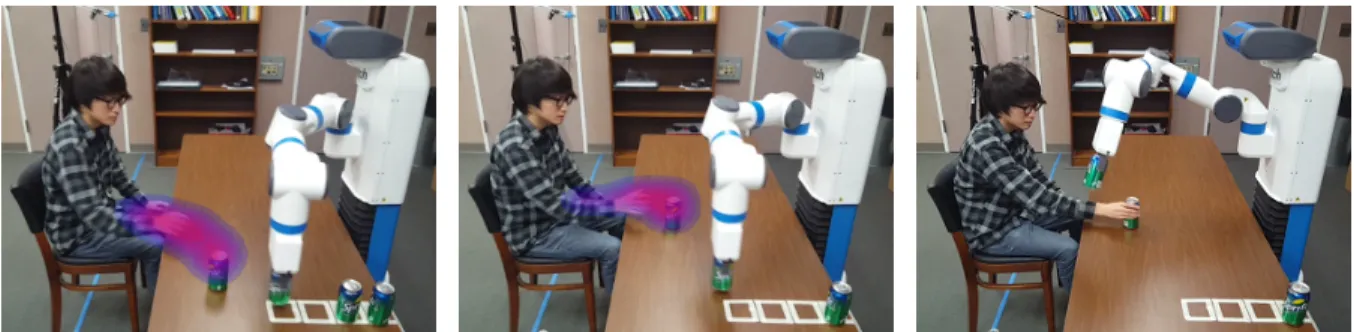
Gaussian error distribution. Our formulation is used to accurately predict future human motions and is integrated with a motion planner for the 7-DOF Fetch robot arm. Compared to prior probabilistic collision detection algorithms based on Gaussian distribution [1], our new method improves the running time by2.6x and improves the accuracy of collision detection by9.7x. . . 8 1.3 The Fetch robot is moving a soda can on a table based on NLP instructions. Initially,
the user gives the “pick and place" command. However, when the robot gets closer to the book, the person says“Don’t put it there” (i.e. negation) and the robot uses our dynamic constraint mapping functions and optimization-based planning to avoid the book. Our approach can generate appropriate motion plans for such attributes. . . . 10 1.4 Probabilistic collision checking with different confidence levels: A collision
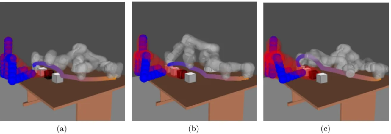
probability less than(1−δCD) implies a safe trajectory. The current pose (i.e. blue spheres) and the predicted future pose (i.e. red spheres) are shown. The robot’s trajectory avoids these collisions before the human performs an action. The higher the confidence levelδCD, the farther the distance between the human arm and the robot trajectory. (a)δCD = 0.90. (b) δCD = 0.95. (c)δCD = 0.99. . . 11 1.5 A human and a robot are simultaneously operating in the same workspace. The robot
arm occludes the camera view and many parts of the human obstacle are not captured by the camera. Three images at the top show the point clouds corresponding to the human in the UtKinect dataset [2] for different camera positions, with the occluded regions in red. The bottom right image highlights the safe motion trajectory between the initial position (blue) and the goal position (yellow). Our safe trajectory is shown in the bottom right as two red curves (with arrows). The occlusion-aware motion planner first moves the arm to reduce the occlusion and then moves it to the goal position. . . 13
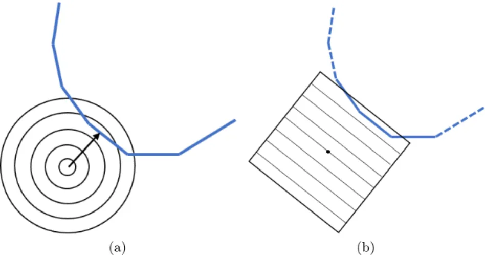
2.1 (a) Contour plots of the bivariate TG distribution. (b) Contour plots of the bounded function Ffor TG are not used in the calculation of collision probability and thereby reduce the running time of collision probability computation. . . 24 2.2 The upper bound of collision probability with uncertainty approximated as Gaussian,
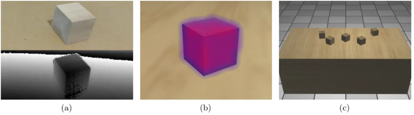
2.3 (a) Speedup of weighted samples (expected) case compared to Monte Carlo (actual) with between 10 to 100 samples (X-axis). (b) Speedup of Truncated Gaussian case, compared to the running time of probabilistic collision detection with a Gaussian. X-axis is the untruncated volume of Gaussian, meaning 100% is the Gaussian and lower value indicates smaller bound. As the truncation boundary shrinks up to 50% of the volume of Gaussian, the algorithm with TG is14x faster times than the algorithm Gaussian distribution. . . 27 2.4 (a) A captured RGBD image. The depth values of the table and the wood block have
noises, even in adjacent frames. The TG noise of each point particle of the wood block contributes to the overall TGMM model. (b) A reconstructed 3D model of a wood block with TGMM, which bounded around the wooden block and more acuracy than Gaussian distribution, which has unbounded probability density function. (c) A reconstructed 3D robot environment with error distributions on the table and the wood blocks. The wood blocks placed in a zig-zag pattern result in 4 narrow passages for the robot. . . 28 2.5 We highlight the benefits of our novel probabilistic collision detection with a Truncated
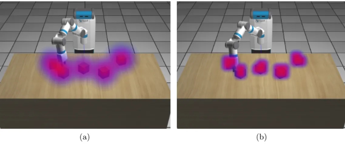
Gaussian error distribution. Our formulation is used to accurately predict the future human motion and integrated with a motion planner for the 7-DOF Fetch robot arm. As compared to prior probabilistic collision detection algorithms based on Gaussian distribution [1], our new method improves the running time by2.6x and improves the accuracy of collision detection by9.7x. . . 29 2.6 The robot trajectory with probabilistic collision detection through narrow passages.
(a) The wood block obstacles are captured by RGBD sensors and its positional errors are modeled with Gaussian distributions. In this case, the planner is unable to compute a path in the narrow passage because of the conservative error bounds on the collision probability. (b) Robot motion planning with probabilistic collision detection under error distribution in the form of TGMM can generate a collision-free robot trajectory that passes through the narrow passage, due to tight bounds. . . 36
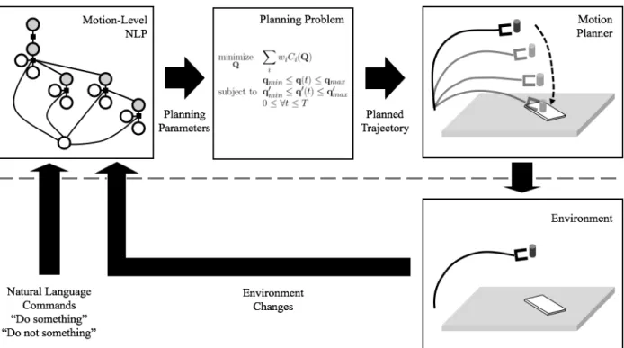
3.1 The overall pipeline of our approach highlighting the NLP parsing module and the motion planner. Above the dashed line (from left to right): Dynamic Grounding Graphs (DGG) with latent parameters that are used to parse and interpret the natural language commands, generation of optimization-based planning formulation with appropriate constraints and parameters using our mapping algorithm. We highlight the high-level interface below the dashed line. As the environment changes or new natural language instructions are given, our approach dynamically changes the specification of the constraints for the optimization-based motion planner and generates the new motion plans. . . 40 3.2 Factor graphs for different commands: In the environment in the right-hand
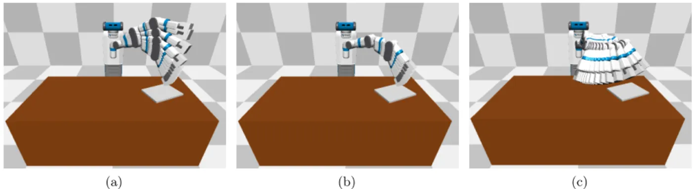
column, there is a table with a thin rectangular object on it. A robot arm is moving a cup onto the table, but we want it to avoid moving over the book when given NLP instructions. (a) The command “Put the cup on the table" is given and the factor graph is constructed (left). Appropriate cost functions for the task are assigned to the motion planning algorithm (middle) and used to compute the robot motion (right). (b) As the robot gets close to the book, another command“Don’t put it there" is given with a new factor graph and cost functions. . . 46 3.3 The simulated Fetch robot arm reaches towards one of the two red objects. (a) When
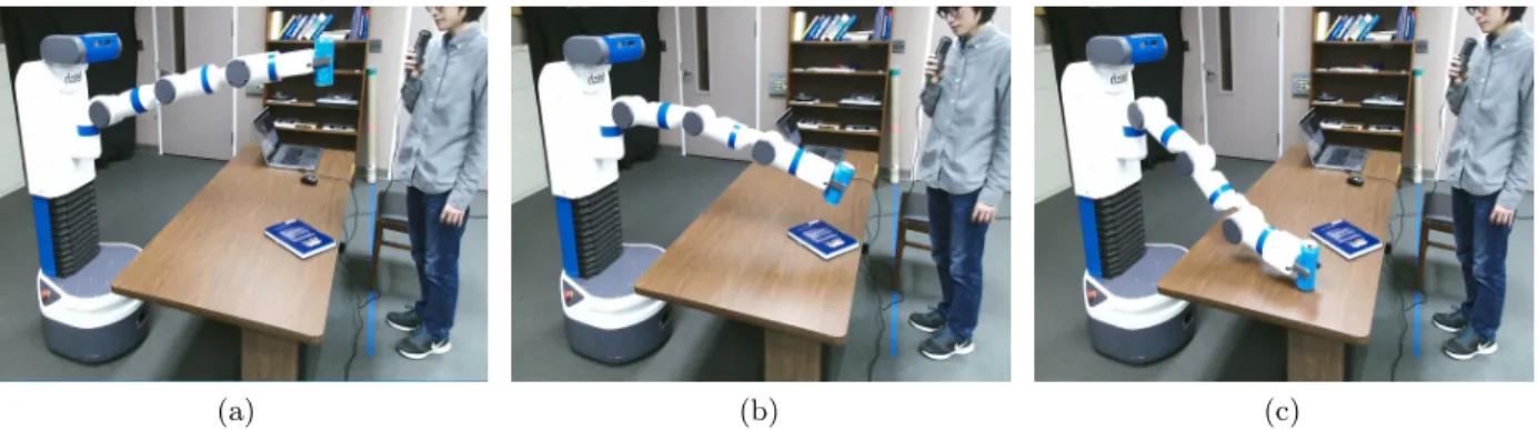
3.4 In this simulated environment, the human instructs the robot to “put the cube on the table” (a). As it approaches the laptop (b), the human uses a negation NLP command “don’t put it there,” so the robot places it at a different location (c). . . 52 3.5 A 7-DOF Fetch robot is operating in a simulated environment avoiding an obstacle.
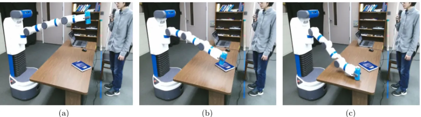
(a) In a traditional optimization-based motion planner, the planner gets stuck at a local minimum. (b),(c) Using natural language commands as guidance, the user guides the robot out of the minimum and towards the goal position. . . 53 3.6 The Fetch robot is taking real-time commands from the human and moves the soda
can on the table. . . 53 3.7 The Fetch robot is moving a soda can on a table based on NLP instructions. Initially,
the user gives the “pick and place" command. However, when the robot gets closer to the book, the person says“don’t put it there” (i.e. negation) and the robot uses our dynamic constraint mapping functions and optimization-based planning to avoid the book. Our approach can generate appropriate motion plans for such attributes. . . . 54
4.1 Overview of our Intention-Aware Planner: Our approach consists of three main components: task planner, trajectory optimization, and intention and motion estimation. . . 63 4.2 Motion uncertainty and prediction: (a) A point cloud and the tracked human
(blue spheres). The joint positions are used as feature vectors. (b) Prediction of next human action and future human motion, where 4 locations are colored according to their probability of next human action from white (0%) to black (100%). Prediction of future motion after 1 second (red spheres) from current motion (blue spheres) is shown as performing the action: move right hand to the second position which has the highest probability associated with it. . . 65 4.3 Human motion prediction results: The result of human motion prediction is
represented by Gaussian distributions for each skeleton joint. The ellipsoid boundaries within which the integral of Gaussian distribution probability is 95% are drawn in red and the human skeleton is shown in blue. Bounding ellipsoids have transparency values that are proportional to the action classifier probability. (a) Undistinguished human action class: This occurs when the classifier fails to distinguish the human action class, generating nearly uniform probability distribution among the action classes. (b) Prediction results when untrained human motion is given: These cases result in larger boundary spheres around the human skeleton. This is because, in the Gaussian Process, the output has a uniform mean and a high variance when the input point is outside the range of the training input data. . . 77 4.4 Performance of human motion prediction: The precision/accuracy of
classifi-cation and regression algorithms are shown in the graphs, with varying input noise. (a) Classification precision versus input noise: We only take the input points where
4.5 Responses to three different human arm movement speeds: While the robot arm moves from left to right, the human moves his arm to block the robot’s trajectory at different speeds. (a) The human arm moves slowly. The robot has enough time to predict the human arm motion, generating the smoothest and the least jerky robot trajectory. (b) As the human moves at a medium speed, the robot predicts the human’s future motion, recognizes that it will block the robot’s path, and therefore changes the trajectory upwards (at t = 0.8s) to avoid the obstacle and generate a smooth trajectory. (c) When the human arm moves faster, the robot trajectory abruptly changes to move upwards (att= 0.8s), generating a less smooth trajectory while still avoiding the human. . . 86 4.6 Different block arrangements: Different arrangements in terms of the positions
of the blocks, results in different human motions and actions. Our planner computes their intent for safe trajectory planning. The different arrangements are: (a)1×4. (b)2×2. (c)2×4. . . 87 4.7 Probabilistic collision checking with different confidence levels: A collision
probability less (1−δCD) implies a safe trajectory. The current pose (i.e., blue spheres) and the predicted future pose (i.e. red spheres) are shown. The robot’s trajectory avoids these collisions before the human performs its action. The higher the confidence level is, the longer the distance between the human arm and the robot trajectory. (a)δCD = 0.90. (b)δCD = 0.95. (c)δCD = 0.99. . . 87 4.8 A 7-DOF Fetch robot is moving its arm near a human, avoiding collisions. (a) While
the robot is moving, the human tries to move his arm to block the robot’s path. The robot arm trajectory is planned without human motion prediction, which may result in collisions and a jerky trajectory, as shown with the red circle. This is because the robot cannot respond to the human motion to avoid collisions. (b) The trajectory is computed using our human motion prediction algorithm; it avoids collisions and results in smoother trajectories. The robot trajectory computation uses collision probabilities to anticipate the motion and compute safe trajectories. . . 88
5.1 A human and a robot are simultaneously operating in the same workspace. The robot arm occludes the camera view and many parts of the human obstacle are not captured by the camera. Three images at the top show the point clouds corresponding to the human in the UtKinect dataset [2] for different camera positions with the occluded regions in red. The bottom right image highlights the safe motion trajectory between the initial position (blue) and the goal position (yellow). Our safe trajectory is shown in the bottom right as two red curves (with arrows). HMPO first moves the arm to reduce the occlusion and then moves it to the goal position. . . 90 5.2 HMPO:Overall pipeline of our human motion prediction and robot motion planning.
We present a new deep learning technique for human motion prediction in occluded scenarios and an optimization-based planning algorithm that accounts for occlusion. 93 5.3 Sample images of original datasets and modifications with occlusion information. (a)
5.4 Benefits of Occlusion-Aware Planning: The top row highlights the point cloud with the dynamic human obstacle, and the regions occluded by robot arms (in red). The bottom row highlights the trajectories computed by different planners when as the robot arm needs to move from right to left: (a) The trajectory is generated by the baseline planner, which does not account for occlusion. When the robot occludes the human, the motion prediction error is high and results in collisions. (b) The robot arm motion is generated by our occlusion-sensitive planner. The arm first moves to reduce the level of occlusion (i.e. a detour) and then reaches the goal to compute a safe trajectory. . . 103 5.5 Average error distance over time for up to 3 seconds between ground truth joint
LIST OF TABLES
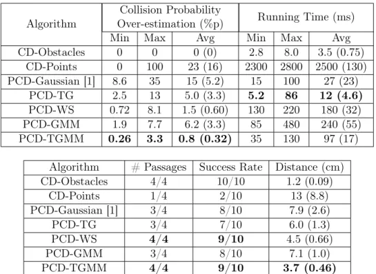
2.1 Performance of probabilistic collision detection algorithms: Evaluated as part of a motion planner with sensor data. The collision probability over-estimation is shown as percent point (%p) with the minimum and maximum over-estimation. The values corresponds to the average over the time of the robot trajectory with standard deviation in parenthesis. The best performance is obtained PCD-TGMM algorithm in terms of collision probability estimation (i.e. tight bounds), successful handling of narrow passages, computing collision-free trajectories, among different algorithms. . . 30
3.1 Planning performances with varying sizes of training data for the scenario in Fig. 3.3 with 21 different NLP instructions. . . 54 3.2 Running time (ms) of our DGG and motion planning modules for each scenario. . . 55 3.3 Examples of DGGs with different configurations of correspondence variables. . . 56 3.4 Examples of DGGs and the latent variables. . . 57 3.5 Examples of DGGs and the latent variables. . . 58
4.1 Performances of action classification and motion regression of ATCRF [5] and our human motion prediction algorithm. As ATCRF algorithm does not predict the variance of motion around the trajectory, the motion regression accuracy cannot be measured on the algorithm. ATCRF uses object affordance annotations as additional information in the learning phase, and we got higher precision and recall with ATCRF than with our algorithm. In terms of motion regression, our algorithm outperformed ATCRF in regression precision. . . 80 4.2 Three different simulation scenarios: Different Arrangements,Temporal Coherence,
andConfidence Level. We consider different arrangements of blocks as well as the confidence levels used for probabilistic collision checking. These confidence levels are used for motion prediction. . . 82 4.3 Performance of our planning algorithm in terms of robot motion simulation. The
use of motion prediction results in a smoother trajectory and we observe up to 4X improvement in our smoothness metric, as defined in Equation (4.12). Our resulting planning algorithm (I-Planner) runs in real-time. . . 83 4.4 Performance of our planning algorithm on a real robot running on a 7-DOF Fetch
robot next to dynamic human obstacles. Our online motion planner computes safe trajectories for challenging benchmarks like “moving cans.” We observe almost 5X improvement in the smoothness of the trajectory due to our prediction algorithm. . . 84
CHAPTER 1
Introduction
Robot motion planning has been extensively studied for many decades [6]. The goal of robot motion planning is to find a trajectory connecting two robot configurations that does not result in collisions with any obstacles. A robot configuration corresponds to a high-dimensional vector describing the robot’s pose. For robot arms, a configuration consists of rotational joint angles. These configurations are used to formulate the configuration space of a robot. The motion planning problem reduces to finding a collision-free one-dimensional path in this high-dimensional space. Robot motion planning has been extensively studies in the field and different solutions based on analytic techniques, sampling-based approaches and optimization-based methods have been proposed [7].
Human-robot interaction (HRI) is an important research area in robotics and has many applica-tions in real-world settings [8]. Traditionally, many industrial robots have been placed away from humans for safety, and this limits their applications. Generally, humans can handle jobs that require better dexterity skills than robots [9, 10]. For some applications, however, it is more efficient for humans and robots to work together while sharing the same workspace. For example, in an assembly job where there are parts to be assembled on a table, a human can assemble parts while a robot arm delivers the parts required for next step of the assembly. If the robot uses a natural language processing module to understand spoken instructions from a human, the person can request that the robot brings the required parts. In such cooperative jobs, humans and robots share the same workspace. In the assembly application, because the human and the robot work on the same table, there is a chance that the robot may collide with the human arms or the human body. Also, the robot should be able to understand the human instructions in terms of natural language processing. If the robot misinterprets the spoken instructions, the robot arm may fail to deliver the correct items, leading to a delay in task completion time.
also understand and predict the human’s intention and avoid the human as a dynamic obstacle. In real-world settings, a major challenge of robot motion planning for cooperation between humans and robots is to deal with uncertainties from many sources. Noisy vision sensors are a source of uncertainty. Depth cameras are widely used for collision avoidance in robot motion planning but result in very noisy inputs. Color cameras have less noise [11], but the noisy input still may cause trouble in terms of vision-related robot motion planning tasks. Human intention and human action prediction are another source of uncertainty. Because of the computation time of robot motion plans and the delay between trajectory planning and trajectory execution, the computed trajectories may collide with a human after the person changes his/her pose from the initial pose that was used by the robot motion planning module. Natural language instructions are yet another source of uncertainty. Spoken commands for robots can be implicit and the robot must sometimes guess the implicit meaning from the context. To overcome these problems related to uncertainty, we need to develop new motion planning algorithms that can handle such uncertainties and also provide realtime performance for human-robot interaction.
1.1 Components of Robot Motion Planning under Uncertainty
Specifically, users can add cost functions or constraints in addition to the smoothness cost and the collision-free constraint to meet specific goals in various real-world settings. For example, when a robot moves a cup filled with water, a user can simply add a constraint that the up-vector of the cup should point in the upward direction. Also, because the robot should not spill the water by moving quickly, a cost function that penalizes high speed or the cup can be added in the objective function.
By taking advantage of the strengths of optimization-based robot motion planning, the basic optimization-based motion planner can be extended in many ways and operated with other techniques, such as predicting future human motions, adding various cost functions for safety and efficiency, and adding constraints related to human motions near robots and natural language commands spoken by humans. A robot motion planner for safe human-robot interaction should consider uncertainties coming from real-world environments. In this section, we discuss some of the components of robot motion planning under uncertainty.
1.1.1 Environment Uncertainty and Collision Probability
Efficient collision detection is important for safe robot motion planning under environmental uncertainties. Previous work in exact collision detection mainly dealt with problems with different variants on input shapes, such as collision detection between rigid convex shapes or collision detection between non-rigid dynamic models [13, 14]. The outputs of these methods are binary values, indicating whether two input shapes are in collision.
When navigating and interacting with real-world objects, robots should gather information about the surroundings and handle environmental uncertainties. Unfortunately, robot cameras or cameras installed around the robot have sensory error, making it difficult to obtain exact shapes and poses of objects in the environment. For example, depth representations captured by depth cameras have errors that correspond to lighting, calibration, or object surfaces [11]. This gives rise to probabilistic collision detection, where the goal is to compute the probability of an in-collision state by modeling the uncertainty using some probabilistic distribution.
where the depth values can vary between consecutive frames due to different noise sources. The dynamic objects in the scene can pose additional problems due to sensor noise and the uncertainties introduced by the objects’ motions. Moreover, Gaussian process dynamical models used to represent human motion [19] have an inherited uncertainty in the Gaussian variances because the central motion is represented using Gaussian means.
Collision probability between robots and obstacles can be used in optimization-based robot motion planner. Collision probability can be used for formulating a hard constraint. For example, a robot motion trajectory should have collision probability between the robot and uncertain surroundings lower than a threshold value (e.g., 0.05).
1.1.2 Understanding Intention from Human Spoken Language
Natural language has been used as an interface to communicate a human’s intent to a robot [20, 21, 22, 23] in the field of human-robot interaction. A key challenge in understanding natural language commands is the uncertainty in natural languages which are typically ambiguous and vague [24]. When the robot misinterprets the natural language commands, it fails to satisfy the human intention. There are many challenges in terms of understanding natural languages for robots. One challenge is that the natural language instructions should be accurately interpreted and represented with grounded linguistic semantics at the motion level, especially considering the surrounding environment and the context. For example, if a human says “Move that to the left” or “Do not move like this,” the robot should learn the correct interpretation of the objectives and constraints, including spatial and motion-based adjectives, adverbs, and negation. Another challenge is that the motion planner should generate appropriate trajectories based on these complex natural language instructions, achieving the intended goal specified by the natural language instructions. To overcome these challenges, the robot motion planner should appropriately set up the motion planning optimization problem based on different motion constraints (e.g., orientation, velocity, smoothness, and avoidance) and compute smooth and collision-free robot trajectories.
1.1.3 Understanding Intention from Human Motion
important for the robots to predict human actions and motions from visual sensor data and to compute collision-free trajectories. Also, human motion prediction makes task completion efficient by predicting the human motion and planning tasks accordingly, when the robots and the humans are sharing the same workspace and arranging the subtasks. For example, in an assembly job where there are parts to be assembled on a table, a human can assemble parts while a robot arm delivers other required parts for the next step. In such cooperative jobs, humans and robots share the same workspace. In the assembly application, because the human and the robot work on the same table, there is a chance that the robot may collide with the human arms or body.
By predicting human motions and intentions, we can achieve improved safety and efficiency in human-robot interaction, computing a safe, collision-free path for the robot to reach its goal configuration and planning subtasks in a way that the entire task is completed as quickly as possible. The robot should not only complete its task but also predict the human’s motion or trajectory to avoid the human as a dynamic obstacle. There is considerable work on human motion prediction and safe trajectory computation. By predicting future human motion trajectory in advance, the robot motion planner can generate a safe motion trajectory for a few seconds in the future by avoiding the predicted human poses. It can also generate an efficient motion trajectory for moving near the human and doing collaborative tasks. Some recent methods to predict human motions from images or videos are based on Convolutional Neural Networks (CNNs) [25, 26, 27, 28] or Recurrent Neural Networks (RNNs) [29, 30].
well when there is sufficient information about prior motion that can be accurately modeled by the underlying motion model. In some scenarios, it is possible to infer high-level human intent using additional information, and thereby perform a better prediction of future human motion. These techniques are used to predict the pedestrian trajectories based on environmental information in 2D domains.
1.1.4 Uncertainty from Robot Occlusions
Robots gather information about the surrounding environment from visual sensors or depth sensors. A head-mounted RGBD camera is a typical device for collaborative robots to observe the workspace. When robots are working with humans sharing the same workspace, the moving parts of the robot may occlude the views of these sensors while robots perform actions with their hands or arms. The input color and depth images may not be able to capture information about many parts of the scenes, including the current position of the human working close to the robot [34, 35, 36]. Such occlusion by parts of a robot can prevent accurate tracking and prediction of the human motion and thereby make it difficult to perform safe and collision-free motion planning. When the robot arm occludes the input images, either the robot should determine whether the human motion can be predicted with high certainty or the robot arm should move so that it does not occlude the field of view of the camera.
To overcome the uncertainty caused by robot occlusions, the robot motion planner should predict what is occuring behind the robot occlusion. Fortunately, robot occlusions in the input color and depth images are known from forward kinematics. From the history of an input image sequence, the robot should predict the unobservable or partially observable humans behind the occlusions or remove the occlusion so that the human can be clearly seen.
1.2 Thesis Statement
Our thesis statement is as follows:
Optimization-based methods and learning algorithms can be combined for safe and efficient motion planning for human-robot interaction and handling uncertainties.
Figure 1.1: A summary diagram of our research. We have developed novel motion planning algorithms that can handle many sources of uncertainty. The center block in the diagram is our main motion planning module, which an optimization solver to find collision-free robot trajectories. The left blocks show novel algorithms that are being used by the motion planner. These include human motion prediction modules and probabilistic collision detection. The right block corresponds to applications that are used to demonstrate the benefits of our novel algorithms.
• Probabilistic collision detection for objects with pose uncertainties: We present probabilistic collision detection algorithms for human motion models and noisy input data. Computing the probability of collision between a robot trajectory and possible future human movements is important because the predicted human motion may be different from the real human motion. Also, because of noises in the depth sensors, the reconstructed environment surrounding the robot is not precise. Probabilistic collision detection deals with computing collision probability when uncertainties of static obstacles captured by robot cameras and predicted dynamic human obstacles are represented by probability distributions. We develop an efficient algorithm when the probability distribution representing uncertainty is given as Gaussian distribution. We also develop efficient algorithms for probabilistic collision detection algorithms for non-Gaussian distributions, where we use more complex statistical models to represent uncertainties.
• Human motion and intention prediction for safe robot motion planning: We present robot motion planning algorithms that can deal with many types of uncertainties. They may come from noisy inputs, unknown human intentions or motions, or spoken natural language instructions. To effectively handle many kinds of uncertainty, we choose optimization-based motion planning algorithms, taking advantage of their versatility.
• Occlusion-aware robot motion planner for partially-visible scenes: We present a prediction model for human motion and intention. As the first step, we develope a human motion prediction algorithm for a human skeletal motion model. This algorithm classifies the type of human action and estimates potential future movements in a short time window; the robot motion planning algorithm uses this information to avoid potential collisions in the future. We also develop a new algorithm based on video input in which the scene may be partially occluded by a robot arm.
1.3 Main Results
In this section, we describe the algorithms to overcome the uncertainty problems in more detail. 1.3.1 Probabilistic Collision Detection
Figure 1.2: We highlight the benefits of our novel probabilistic collision detection with a Truncated Gaussian error distribution. Our formulation is used to accurately predict future human motions and is integrated with a motion planner for the 7-DOF Fetch robot arm. Compared to prior probabilistic collision detection algorithms based on Gaussian distribution [1], our new method improves the running time by2.6x and improves the accuracy of collision detection by 9.7x.
and highlight the benefits over prior methods for probabilistic collision detection. We evaluate the performance of these methods on synthetic and real-world datasets captured using depth cameras. Furthermore, we show that our efficient probabilistic collision detection algorithm can be used for real-time robot motion planning of a 7-DOF manipulator in tight scenarios with depth sensors. Some novel components of our work include:
• A novel method to perform probabilistic collision detection for TG Mixture Models based on appropriately formulating the vector field and computing an upper bound using a divergence theorem on the resulting integral. Moreover, we present an efficient method to evaluate this bound for convex and non-convex shapes.
• We show that TG outperforms normal Gaussian, and Truncated Gaussian Mixture Model (TGMM) outperforms Gaussian Mixture Model (GMM). In practice, probabilistic formulation is less conservative than prior methods and results in 5−9× better accuracy in terms of collision probability computation (Table 1).
• We have combined our probabilistic collision formulation with an optimization-based realtime robot motion planner that accounts for positional uncertainty from depth sensors. Our modified planner is less conservative in terms of computing paths in tight scenarios.
In Chapter 2, we present an efficient algorithm to compute tight upper bounds of collision probability between two objects with positional uncertainties with error distributions represented with non-Gaussian forms. Our approach can handle noisy datasets from depth sensors with distributions that may correspond to Truncated Gaussian, Weighted Samples, or Truncated Gaussian Mixture Model. We derive tight probability bounds for convex shapes and extend them to non-convex shapes using hierarchical representations. We highlight the benefits of our approach over prior probabilistic collision detection algorithms in terms of tighter bounds (10x) and improved running time (3x). Moreover, we use our tight bounds to design an efficient and accurate motion planning algorithm for a 7-DOF robot arm operating in tight scenarios with sensor and motion uncertainties.
1.3.2 Motion Planning using NLP Instructions
(a) (b) (c)
Figure 1.3: The Fetch robot is moving a soda can on a table based on NLP instructions. Initially, the user gives the “pick and place" command. However, when the robot gets closer to the book, the person says “Don’t put it there” (i.e. negation) and the robot uses our dynamic constraint mapping functions and optimization-based planning to avoid the book. Our approach can generate appropriate motion plans for such attributes.
Graphs(DGG) to parse and interpret the commands and to generate the constraints. Our formulation includes the latent parameters in the grounding process, allowing us to model many continuous variables in our grounding graph. Furthermore, we present a new dynamic constraint mapping that takes DGG as the input and computes different constraints and parameters for the motion planner. The appropriate motion parameters are speed, orientation, position, smoothness, repulsion, and avoidance. The final trajectory of the robot is computed using a constraint optimization solver. Overall, our approach can automatically handle complex natural language instructions corresponding to spatial and temporal adjectives, adverbs, superlative and comparative degrees, negations, etc. Compared to prior techniques, our overall approach offers the following benefits:
• The inclusion of latent parameters in the grounding graph allows us to model continuous variables that are used by our mapping algorithm. Our formulation computes the dynamic grounding graph based on conditional random fields.
• We present a novel dynamic constraint mapping used to compute different parametric con-straints for optimization-based motion planning.
We highlight the performance of our algorithms in a simulated environment and on a 7-DOF Fetch robot operating next to a human. Our approach can handle a rich set of natural language commands and can generate appropriate paths. These include complex commands such as picking (e.g.,“Pick up a red object near you"), correcting the motion (e.g.,“Don’t pick up that one"), and
negation (e.g., “Don’t put it on the book").
In Chapter 3, we present an algorithm for combining natural language processing (NLP) and fast robot motion planning to automatically generate robot movements. Our formulation uses a novel concept called Dynamic Constraint Mapping to transform complex, attribute-based natural language instructions into appropriate cost functions and parametric constraints for optimization-based motion planning. We generate a factor graph from natural language instructions called the Dynamic Grounding Graph (DGG), which takes latent parameters into account. The coefficients of this factor graph are learned based on conditional random fields (CRFs) and are used to dynamically generate the constraints for motion planning. We map the cost function directly to the motion parameters of the planner and compute smooth trajectories in dynamic scenes. We highlight the performance of our approach in a simulated environment and via a human interacting with a 7-DOF Fetch robot using intricate language commands including negation, orientation specification, and distance constraints.
1.3.3 Human Intention-aware Robot Motion Planner
(a) (b) (c)
We present a novel high-DOF motion planning approach to compute collision-free trajectories for robots operating in a workspace with human obstacles or human-robot cooperation scenarios (I-Planner). Our approach is general and doesn’t make assumptions about the environment or the human actions. We track the positions of the human using depth cameras and present a new method for human action prediction using a combination of classification (to predict the type of human motion) and regression (to predict the actual future human motion) methods. Given the sensor noises and prediction errors, our online motion planner uses probabilistic collision checking to compute a high-dimensional robot trajectory that tends to compute safe motions in the presence of uncertain human motion. In contrast to prior methods, the main benefits of our approach include:
1. A novel data-driven algorithm for intention and motion prediction, given noisy point cloud data. Compared to prior methods, our formulation can account for a lot of noise in skeleton tracking in terms of human motion prediction.
2. An online high-DOF robot motion planner for efficient completion of collaborative human-robot tasks that uses upper bounds on collision probabilities to compute safe trajectories in challenging 3D workspaces. Furthermore, our trajectory optimization based on probabilistic collision checking results in smoother paths.
We highlight the performance of our algorithms in a simulator with a 7-DOF KUKA arm and in a real-world setting with a 7-DOF Fetch robot arm in a workspace with a moving human performing cooperative tasks. We have evaluated its performance in some challenging or cluttered 3D environments where the human is close to the robot and moving at varying speeds. We demonstrate the benefits of our intention-aware planner in terms of computing safe trajectories in these scenarios. A preliminary version of this paper was published [36]. Compared to [36], we improve the human motion prediction algorithm using depth sensor data. We present a mathematical analysis of the robustness of our prediction algorithm and highlight its benefits and improved accuracy for challenging scenarios. We also analyze the performance of our algorithm with varying human motion speeds.
Our intention-aware online planning algorithm uses the learned database to compute a reliable trajectory based on the predicted actions. We represent the predicted human motion using a Gaussian distribution and compute tight upper bounds on collision probabilities for safe motion planning. We also describe novel techniques to account for noise in human motion prediction. We highlight the performance of our planning algorithm in complex simulated scenarios and real-world benchmarks with 7-DOF robot arms operating in a workspace with a human performing complex tasks. We demonstrate the benefits of our intention-aware planner in terms of computing safe trajectories in such uncertain environments.
1.3.4 Occlusion-aware Robot Motion Planner
human motion in the presence of obstacles and occlusions; (2) plan a robot’s motion while taking into account the occlusion and the uncertainty in the motion prediction.
• Human Motion Prediction in Occluded Scenarios: We present a neural network that uses not only the features from RGBD images, but also features related to occlusion. Our deep learning-based approach predicts the human motion in such occluded scenarios. We use CNNs for feature extraction from RGBD images and feature extraction for robot occlusion. Moreover, we use ResNet-18 [37] to extract visual features from color images with occluded regions. Our learning algorithm classifies the human action and generates the predicted human motion using a skeleton-based human model. We add occluded images of robot scenes to existing RGBD human action prediction datasets [2, 3, 4]. We use these augmented datasets to train and evaluate the performance of our human motion prediction algorithm in the presence of occlusion. In practice, our action classification algorithm improves the prediction accuracy by 63%over prior classification algorithms [3].
• Occlusion-Aware Motion Planning: We present a realtime planning algorithm to compute a safe trajectory for a robot in occluded scenes with human obstacles. We use an optimization-based planning framework and add the occlusion constraints in the objective function. Our planner tends to compute collision-free paths and ensures that the human region in the camera image is not occluded by the robot. We have evaluated our planner in complex environments with robots operating close to the human. In practice, our algorithm improves the overall accuracy, measured using error distance between the ground-truth and the predicted human joint positions, by38%.
We use three human action RGB-D datasets and augment them with occlusion characteristics for training and validation. We highlight the performance of the overall approach (HMPO) in complex environments. We released our source code for augmenting the datasets athttps://github.com/ jsonpark/occlusion
CHAPTER 2
Efficient Probabilistic Collision Detection
Efficient collision detection is an important problem in robot motion planning, physics-based simulation, and geometric applications. Earlier work in collision detection focused on fast algorithms for rigid convex polytopes and non-convex shapes and later extended to non-rigid models [13, 14]. Most of these methods assume that an exact geometric representation of the objects is known in terms of triangles or continuous surfaces [38] and the output of collision query is a simple binary outcome.
As robots navigate and interact with real-world objects, we need algorithms for motion planning and collision detection that can handle environmental uncertainty. In particular, robots operate with sensor data, and it is hard to obtain an exact shape or pose of an object. For example, depth cameras are widely used in robotics applications and the captured representations may have errors that correspond to lighting, calibration, or object surfaces [11]. This gives rise to probabilistic collision detection, where the goal is to compute the probability of in-collision state by modeling the uncertainty using some probabilistic distribution.
In many applications, it is necessary to use non-Gaussian models for uncertainties [39]. These include Truncated Gaussian with bounded domains for sensory noises [40, 41] to represent the position uncertainties for a point robot position [42]. Other techniques model the uncertainty as a Partially Observable Markov Decision Process (POMDP) [43, 44].
2.1 Related Work
We give a brief overview of prior work on probabilistic collision detection. 2.1.1 Probabilistic Collision Detection for Gaussian Errors
avoid collisions with cars or pedestrians. Xu et al. [18] use Linear-Quadratic Gaussian to model the stochastic states of car positions on the road. Collision detection under uncertainty is performed by computing the Minkowski sum of Gaussian ellipse boundary and the rectangular car model and checking for overlap with other rectangular car model. Park et al. [1] present an efficient algorithm to compute an upper bound of the collision probability with Gaussian error distributions [1]. This approach can be extended to Truncated Gaussian because the probability density function (PDF) of a Truncated Gaussian inside its ellipsoidal domain has the same value as that of the PDF of a Gaussian. Therefore, the upper bound computed using [1] also holds for Truncated Gaussian error distributions, but the bound is not tight. Moreover, a Truncated Gaussian distribution has a bounded ellipsoidal domain and the integral computations outside the domain can be omitted. As compared to this approach, our new algorithm improves the tightness of the upper bound and the running time, as shown in Section 5.
2.1.2 Probabilistic Collision Detection for Non-Gaussian Errors
The collision probability for non-Gaussian error distributions can be computed with Monte Carlo sampling [45]. However, these methods are much slower (10−1000 times), as compared to probabilistic algorithms that use Gaussian forms of error distributions [1]. Althoff et al. [46] use a non-Gaussian probability distribution model on the future states of other cars on the road, based on their positions, speeds, and road geometry. They use a 2D grid discretization of the state space and Markov chain to compute the probability that a car belongs to a cell. This method assumes that the environment sensors has no noise. Lambert et al. [47] use a Monte Carlo approach, taking advantage of the probability density function represented as a Gaussian. Other methods have been proposed for point clouds using classification [17] or Monte-Carlo integration [48]. Approaches based on Partially Observable Markov Decision Processes (POMDPs) make efficient decisions about the robot actions in a partially observable state in an uncertain environment [39, 49]. Some applications using POMDPs [50] have been developed to avoid collisions in an uncertain environment, where the uncertainty is represented with a non-Gaussian probability distribution. Our approach for non-Gaussian distributions is different and complementary with respect to these methods.
2.1.3 Probabilistic Collision Detection: Applications
error is represented by a Gaussian distribution that propagates over a discretized time domain. The upper bound on the collision probability is computed on the Gaussian positional error with an erf(·) function for a point obstacle. Fisac et al. [52] compute the collision probability between the dynamic human motion and a robot, and use that value for robot motion planning in the 3D workspace. This algorithm models the human motion based on human dynamics, discretizes the 3D workspace into smaller grids, and integrates the cell probabilities over the volume occupied by the robot. Probabilistic collision detection for a Gaussian error distribution [1] has been used for optimization-based robot motion planning. The collision constraint used in the optimization formulation is that the collision probability should be less than 5%at any robot configuration in the resulting trajectory. However, with Gaussian error distributions, the upper bound of collision probability is rather conservative. As a result, these approaches do not work well in tight spaces or narrow passages.
2.2 Overview
In this section, we introduce the terminology used in the paper and give an overview of our approach. Our algorithm is designed for environments, where the scene data is captured using sensors and only partial observations are available. In this case, the goal is to compute the collision probabilitybetween two objects, when one or both objects are represented with uncertainties and some of the input information such as positions or orientations of polygons or point clouds are given as probability distributions
2.2.1 Probabilistic Collision Detection
and pB, can be formulated as
pcol=
˚
A
˚
B
I((A+A)∩(B+B)6=∅)
p(A)p(B)dAdB, (2.1)
A∼PA, B ∼PB, (2.2)
where I(·) is an indicator function which yields 1 if the condition is true and 0 otherwise,Aand
B are the displacement vectors for Aand B with the probability distributionPA and PB, and L denotes the Minkowski sum operator between two shapes.
To generalize, we shift only one object Aby=A−B which follows a probabilistic distribution
PAB, instead of shifting the two objects separately by A andB. Because of the independence of probabilistic distributionsPA andPB, the convolutionPAB of PA and PB can be expressed as:
fAB(x) =
˚
y
fA(y)fB(x−y)dy, (2.3)
wherefAB,fA,fB are the probability density functions of PAB,PA,PB, respectively. 2.2.2 Probabilistic Collision Detection for Gaussian Error
The general probabilistic collision detection problem is hard to solve, when the error distributions
PAand PB have any arbitrary form. The convolution operator in (Equation (2.3)) can be hard to formulate in the general case. However, it is known that the convolution of two Gaussians is also Gaussian. This generalizes the use of two error distributions into one, yielding the following:
pcol=
˚
I
(A+)MB)6=∅
p()d (2.4)
=
˚
I∈(−A)MBp()d, ∼PAB. (2.5)
Gaussian along the minimum displacement vector direction. In practice, the resulting bounds are conservative.
2.3 Truncated Gaussian Mixture Model Error Distribution
In this section, we present an efficient algorithm for Truncated Gaussian Mixture Model (TGMM) error distributions, which is a more general type of noise model for robotics applications. To compute the collision probability for TGMM, we first introduce the solutions for simpler error distributions corresponding to Truncated Gaussian (TG) and Weighted Samples (WS). We combine these two algorithms to design an algorithm for a multiple Truncated Gaussian error distribution model. 2.3.1 Truncated Gaussian Mixture Models
A TGMM consists of multiple Truncated Gaussian (TG) distributions, each distribution with a truncated domain. The probability density function of a TG,fT G, can be formulated as:
fT G(x;µ,Σ, r) =
1
ηg(x;µ,Σ) (x−µ)TΣ
−1(x−µ)≤r
0 otherwise
, (2.6)
where g is the probability density function of a Gaussian, µ is the mean, Σ is the variance, r is the radius of bound in the coordinates of the principal axes, and η is the truncation rate used to compensate the loss of truncated volume of probability outside the bound. A TGMM consists of
nTGs with multiple weights wi. The probability density function of the TGMM,fT GM M, can be formulated using the definition of fT G in Equation (2.6), as:
fT GM M(x) = n
X
i=1
wifT G(x;µi,Σi, ri), n
X
i=1
wi = 1. (2.7)
As the radii of TGs decrease and converge to zero, the probability model behaves like a discrete probability distribution, which we call Weighted Samples (WS). The WS is a discrete probability distribution, formulated as:
P(X=xi) =wi, n
X
i=1
wi= 1 (2.8)
2.3.2 Collision Probability for Truncated Gaussian
The TG is a Gaussian with a specific form of bounded domain. The bounded domain for 3D Truncated Gaussian is an ellipsoid, centered at the Gaussian mean and having the same principal axes as those of Gaussian variances. The TG is formulated with a collision probability function as
pcol =
˚
VAB
fT G(x;µ,Σ, r)dx, (2.9)
where VAB = −ALB, fT G is the probability density function for TG, µ is the mean, Σ is the variance,r is the radius of bound in the coordinates of the principal axes, andη is the normalization constant used to compensate the loss of truncated volume of probability outside the bound. Because
fT G has the value of a Gaussian multiplied byη inside the boundary, the integral volume becomes −AL
B∩VT G, where VT G is the valid volume of Truncated Gaussian. The collision probability corresponds to
pcol = 1
η ˚
VAB∩VT G
fT G(x;µ,Σ, r)dx. (2.10)
The TG has its center at µand principal axes with different lengths determined byΣ. To normalize the function, a transformationT = Σ−1/2−µI is applied to the coordinate system, which changes Equation (2.10) to
pcol = 1
ηdet Σ
˚
V0 AB∩VT G0
fT G(x;0, I, r)dx, (2.11)
VAB0 =T(VAB), VT G0 =T(VT G). (2.12)
In the transformed coordinate system, VT G0 is a sphere of radiusr.
computation of collision probability reduces to the computation of the integral
˚
V0
g(x;0, I)dx, (2.13)
whereV0=VAB0 ∩VT G0 , and g(·) is the Gaussian probability density function.
From the convexity of VAB0 , the minimum distance vector d0 between the origin andVAB0 can be computed by using the GJK algorithm [53] betweenA0 andB0, which are transformed from A
andB byT. Letn0d be the unit directional vector ofd’. Then, by the Cauchy-Schwarz inequality (x·n0d)2 ≤ kxk2, the integral is bounded by
pcol ≤
˚
V0 1 √
8π3exp
−1 2(x·n
0 d)2
dx. (2.14)
The integrand of the upper bound term behaves as a 1D Gaussian function instead of being the 3D function. We use the divergence theorem to compute the upper bound on collision probability (2.14).
˚
V0
div(F)dV =
‹
S0
(F·nS)dS, (2.15)
whereF is a vector field,S0 is the surface ofV0,dSis an infinitesimal area for integration, andnS is the normal vector of dS. This converts the volume integral to a surface integral. Let’s define Fas
F(x) = 1 2π
1 +erf
x·n0d √
2
n0d, (2.16)
where erf(·)is the 1D Gaussian error function. Note thatF is a vector field with a single directionn0d. The directional derivative of F(x) along any directional vector orthogonal to n0d is zero because F varies only alongn0d. The divergence ofF thus becomes(∂F/∂n0d), and this is equal to the function in Equation (2.14).
We apply the divergence theorem in Eqation (2.15) to the volume integral on V0 in Equation (2.14). Note that V0 is a 3D volume intersection between a non-convex polytope VAB0 and a ball
decomposed into two parts and bounded by the sum of two components as
X
i
‹
4S0 i
(F·n0i)dS+
‹
S0 T G
(F·nS)dS, (2.17)
where Si0 is thei-th triangle of VAB0 inside VT G0 , n0i is the normal vector of 4Si0, and ST G0 is the spherical boundary of VT G0 outside of a plane defined by d0. The second term corresponds to the spherical domain of the normalized Truncated Gaussian with the truncation rate η. The magnitude of F on the spherical boundaryVT G0 is upperly bounded by (1−η), because it is the cumulative distribution function on the boundary. The surface area of ST G0 is less thanπ||d0||2. This can be used to express a bound based on the following lemma.
Lemma 2.3.1. The collision probability represented in a volume integral is upperly bounded by a surface integral as follows:
pcol =
˚
V0
g(x;0, I)dx (2.18)
≤X i
‹
4Si
(F·ni)dS+π(1−η)||d0||2, (2.19)
where F is a vector field in 3D space whose maximum magnitude is1/π, andSi is the i-th triangle of VAB0 that is inside VT G0 .
Because the error function integral over a triangle domain is hard to compute, the upper bound on the integral is evaluated as
X
i
‹
4Si
(F·ni)dS (2.20)
≤X i
max
j=1,2,3F(Sij)·ni
Area(4Si), (2.21)
(a) (b)
Figure 2.1: (a) Contour plots of the bivariate TG distribution. (b) Contour plots of the bounded function F for TG are not used in the calculation of collision probability and thereby reduce the running time of collision probability computation.
Figure 2.2: The upper bound of collision probability with uncertainty approximated as Gaussian, Gaussian Mixture, and Weight Samples. The X-axis is the true collision probability computed using Monte Carlo methods, and Y-axis is the computed probability using different methods. The computed upper bound for Gaussian Mixture and Weights Samples are closer to the ground truth/exact answer, than that for a single Gaussian approximation. The collision probability over-estimation with TGMM is reduced by 90%, compared to the one with Gaussian distribution.
2.3.3 Efficient Evaluation of the Integral
for collision probability is bounded by the cube, primitives outside the cube can be ignored in terms of calculating the upper bound of collision probability. Limiting the computation to the truncated primitives can accelerate the running time.
In order to perform this computation for non-convex primitives, we construct bounding volume hierarchies (BVHs) forAandB, with each bounding volume being an oriented bounding box. During the traversal of the BVHs, the oriented bounding boxes are first transformed byT. The transformed bounding volumes are still convex primitives, the surface integral can be obtained using Equation (2.21).
2.3.4 Error Distribution as Weighted Samples
For the weighted samples, the probability distributions are given by multiple points pi with weights wi, yielding a discrete probability distribution, as described in Equation (2.8). The collision probability of Equation (2.4-2.5) for the weighted samples is given as:
pcol = n
X
i=1
wiI
xi ∈(−A)
M B
,
n
X
i=1
wi= 1, (2.22)
wherewi is weight andI(·)is the indicator function which yields1if the statement inside is true or0 otherwise. The formulation is the weighted average ofncollision detection results. A simple solution to this problem is to run exact collision detection algorithmsn times and sum up the weights of in-collision cases. However, this results in anO(n)and we use BVHs to accelerate that computation.
We have the bounding volumes for the weighted samples and the two polyhedra. When there is no overlap between the bounding boxes, it implies that there is no collisions between two shapes for all weighted samples in the corresponding bounding volume. If the bounding volumes overlap, there may be a collision for each weighted samples, and the bounding volumes of the children are checked recursively for collisions. Each of these bounding volume checks can be performed in O(1)time.
probability.
In order to reduce the time complexity for more complex forms of error distributions, we construct a Bounding Volume Hierarchy (BVH) [13] over the error distributions of mixture models with Oriented Bounding Boxes (OBBs) [54] and apply the collision probability algorithm on its nodes, which are convex primitives. We construct a BVH for the weighted samples and for Truncated Guassian Mixture Models inO(n)time complexity. The BVH is generated from the root node that contains every Truncated Gaussians, and the bounding volume for the root node is computed by minimizing the volume of the oriented bounding box. Next, the bounding volume is split at the center along the longest edge and two child BVH nodes are generated, each containing appropriate samples. This process is repeated till the leaf nodes.
2.3.5 Error Distribution as Truncated Gaussian Mixture Models For TGMM the probability distribution is given as:
pcol = n
X
i=1
wi
˚
VAB
ηifT GM M(x;µi,Σi, ri)dx, (2.23)
wherenis the number of Truncated Gaussians (TGs),wi is the weight of each TG, andµi,Σi andri are the mean, variance and radius of TGs, respectively. The overall algorithm for TGMM is obtained by combining the two previous algorithms. A change from the algorithm for weighted samples is that the BVH is constructed for n TGs with their ellipsoid bounds instead of the point samples. The details of algorithms and pseudo-codes are given in the appendix [55].
2.4 Performance and Analysis
In this section, we describe our implementation and highlight the performance of our probabilistic collision detection algorithms on synthetic and real-world benchmarks. Furthermore, we measure the upper bound of collision probabilities and speedups for algorithms with different noise distributions, compared to the exact collision probability computed by Monte Carlo method.
2.4.1 Probabilistic Collision Detection: Performance
(a)
(b)
Figure 2.3: (a) Speedup of weighted samples (expected) case compared to Monte Carlo (actual) with between 10 to 100 samples (X-axis). (b) Speedup of Truncated Gaussian case, compared to the running time of probabilistic collision detection with a Gaussian. X-axis is the untruncated volume of Gaussian, meaning 100% is the Gaussian and lower value indicates smaller bound. As the truncation boundary shrinks up to 50% of the volume of Gaussian, the algorithm with TG is14x faster times than the algorithm Gaussian distribution.
collision probability over-estimation.
(a) (b) (c)
Figure 2.4: (a) A captured RGBD image. The depth values of the table and the wood block have noises, even in adjacent frames. The TG noise of each point particle of the wood block contributes to the overall TGMM model. (b) A reconstructed 3D model of a wood block with TGMM, which bounded around the wooden block and more acuracy than Gaussian distribution, which has unbounded probability density function. (c) A reconstructed 3D robot environment with error distributions on the table and the wood blocks. The wood blocks placed in a zig-zag pattern result in 4 narrow passages for the robot.
not performed when the truncation boundary of TGs does not overlap with the Minkowski sum of bounding volumes for the two objects. On the other hand, for Gaussian distribution there are no truncation boundaries and the BVH traversal continues. Thereore, we observe speedup with TGs over Gaussian, as shown in Figure 1 and Table 1. Overall, the speedup depends on the range of truncation. A smaller truncation boundary results in faster performance of our probabilistic collision detection algorithm.
2.4.2 Sensor Noise Models for Static Obstacles
Figure 2.5: We highlight the benefits of our novel probabilistic collision detection with a Truncated Gaussian error distribution. Our formulation is used to accurately predict the future human motion and integrated with a motion planner for the 7-DOF Fetch robot arm. As compared to prior probabilistic collision detection algorithms based on Gaussian distribution [1], our new method improves the running time by 2.6x and improves the accuracy of collision detection by9.7x. and variance of a Truncated Gaussian are the same. The truncation rate η with which the integral in the ellipsoidal boundary is set to 90% in our benchmarks. With the fixed truncation rate, the positional error is bounded around the wooden blocks, unlike the positional error represented by Gaussians with an unbound domain. The confidence levelδ is related to the robot motion planner, constraining that the collision probability between the robot and the objects should be less than 1−δ at any robot trajectory point. In our benchmarks,δ is set to 95%.
Figure 2.4 shows a captured depth image, a noise distribution modeled using Truncated Gaussian Mixture Model, and a reconstructed 3D environment with noises. The pixels on the boundary of the object have higher variance in terms of noise. So, the Truncated Gaussian Mixture noise model may have some Gaussians with higher variance. A principal axis for those boundary pixels is perpendicular to the boundary direction.
2.4.3 Robot Motion Planning
Algorithm
Collision Probability
Over-estimation (%p) Running Time (ms)
Min Max Avg Min Max Avg
CD-Obstacles 0 0 0 (0) 2.8 8.0 3.5 (0.75)
CD-Points 0 100 23 (16) 2300 2800 2500 (130) PCD-Gaussian [1] 8.6 35 15 (5.2) 15 100 27 (23)
PCD-TG 2.5 13 5.0 (3.3) 5.2 86 12 (4.6)
PCD-WS 0.72 8.1 1.5 (0.60) 130 220 180 (32)
PCD-GMM 1.9 7.7 6.2 (3.3) 85 480 240 (55)
PCD-TGMM 0.26 3.3 0.8 (0.32) 35 130 97 (17) Algorithm # Passages Success Rate Distance (cm)
CD-Obstacles 4/4 10/10 1.2 (0.09)
CD-Points 1/4 2/10 13 (8.8)
PCD-Gaussian [1] 3/4 8/10 7.9 (2.6)
PCD-TG 3/4 7/10 6.0 (1.3)
PCD-WS 4/4 9/10 4.5 (0.66)
PCD-GMM 3/4 8/10 7.1 (1.0)
PCD-TGMM 4/4 9/10 3.7 (0.46)
Table 2.1: Performance of probabilistic collision detection algorithms: Evaluated as part of a motion planner with sensor data. The collision probability over-estimation is shown as percent point (%p) with the minimum and maximum over-estimation. The values corresponds to the average over the time of the robot trajectory with standard deviation in parenthesis. The best performance is obtained PCD-TGMM algorithm in terms of collision probability estimation (i.e. tight bounds), successful handling of narrow passages, computing collision-free trajectories, among different algorithms.
captured by the two sensors are used to reconstruct the environment. In this case, the reconstructed table surface and wood block obstacles have errors due to the noise in the depth sensors. Figure 2.4 (c) shows the reconstructed environment from depths sensors and the error distributions around the obstacles. The robot arm’s task is to move a wood block, drawing a zig-zag pattern that passes through the narrow passages between the wood blocks. The objective is to compute a robot trajectory that minimizes the distance between the robot’s end-effector and the table, and not resulting in any collisions. The following metrics are used to evaluate the performance:
• Collision Probability Over-estimation: Because we compute the upper bounds of collision probability in our algorithm, we measure the extent of collision probability over-estimation, the gap between the upper bound of collision probability and the actual collision probability.
• # Passages: The successful number of passes the robot makes between wood blocks.
• Success Rate: The number of collision-free trajectories, out of the total number of trajec-tory executions. For each execution, the wood block’s positions are set following the error distribution.
• Distance: The distance between the robot’s end-effector and the table. A lower value is better, as it implies that the robot can interact with the environment in close proximity.
The collision probability over-estimation, running time, distance values are measured for robot poses of every 1/30 seconds over the robot trajectories.
We compare the performances of 5 different collision detection algorithms: exact collision detection with static obstacles without environment uncertainties (CD-Obstacles), exact collision detection with point clouds (CD-Points), probabilistic collision detection with Gaussian errors (PCD-Gaussian) [1], PCD with Truncated Gaussian (PCD-TG), PCD with weighted samples (PCD-WS), and PCD with Truncated Gaussian Mixture Model (PCD-TGMM). The weighted samples are drawn from the TGMMs. For each TG distribution, one sample is drawn from its center. Other samples are drawn from three icosahedrons with the same centers and different radii by uniformly dividing the truncation radius.