Application of Bioimage Informatics to Quantification of Focal Adhesions and Invadopodia
Matthew E. Berginski
A dissertation submitted to the faculty of the University of North Carolina at Chapel Hill in partial fulfillment of the requirements for the degree of Doctor of Philosophy in the Depart-ment of Biomedical Engineering.
Chapel Hill 2013
Approved by:
Shawn M. Gomez, Eng.Sc.D. James E. Bear, Ph.D.
Abstract
MATTHEW E. BERGINSKI: Application of Bioimage Informatics to Quantification of Focal Adhesions and Invadopodia.
(Under the direction of Shawn M. Gomez, Eng.Sc.D..)
The development of the ability to fluorescently label functional proteins and visualize their subcellular localization using microscopy in living cells, has made it possible to study a wide range of single cell phenomena. To understand the results of imaging assays, cell biologists have used manual methods for determining the quantitative properties of the cellular structures visualized fluorescent microscopy. As the quantity and complexity of the images that can be collected using fluorescence microscopy has increased, a new subfield of Bioinformatics has developed, named Bioimage Informatics, which specializes in adapting and developing new methods to quantify the image sets resulting from biological assays.
Acknowledgments
This work would not have been possible without the support of my adviser, Shawn Gomez. His door has always been open when I needed to discuss this work and he has always provided advice when I’ve needed it. I can also thank Shawn for introducing me to Eric Vitriol and Klaus Hahn who saw the need for methods quantify Focal Adhesions. I can also thank Eric for introducing my work to Jim Bear, who provided me the opportunity to continue to develop the Focal Adhesion analysis methods and work in his lab. I am would also like to thank the rest of my committee, Anne Taylor, Glenn Walker and Marc Niethammer, for their feedback and advice. I would also like to acknowledge the Bioinformatics training grant, the UCRF fund and the NSF Graduate Research Fellows Program for providing funding.
I would also like to thank the members of the Gomez lab, Kwangbom Choi, Jen Staab, Alicia Midland, Janet Doolittle, Ke Xu, Dan Oreper and Kyla Lutz who have provided valu-able feedback about my work. The members of the Bear lab, David Roadcap, Sarah Creed, Shelly Cochran, Keefe Chan, Emma Wu and Sreeja Asokan, also provided many hours of training and feedback in the lab. My fellow students in the Bioinformatics training program have also played an important role in my development as a scientist.
Table of Contents
List of Figures . . . viii
1 Introduction . . . 1
1.1 Bioimage Informatics . . . 2
1.1.1 Methods Overview . . . 3
1.1.2 High-throughput Image Analysis in Screening . . . 4
1.1.3 High-content Image Analysis in Cell Biology . . . 6
1.2 Thesis Contributions . . . 7
2 High-resolution Quantification of Focal Adhesion Dynamics in Living Cells . . 9
2.1 Introduction . . . 9
2.2 Results . . . 11
2.2.1 Quantitative Analysis of Focal Adhesion TIRF Images . . . 11
2.2.2 Kinetics of FA Assembly and Disassembly . . . 13
2.2.3 Spatial Properties of FA Assembly and Disassembly . . . 17
2.2.4 Analysis of EGFP-labeled FAK adhesions . . . 17
2.3 Methods . . . 21
2.3.1 Cell Culture . . . 21
2.3.2 Microscopy . . . 24
2.3.3 Image Processing . . . 25
2.3.4 FA Tracking . . . 26
2.3.6 Results Filtering . . . 30
2.3.7 Parameter Testing . . . 30
2.3.8 Software Testing . . . 31
2.3.9 Statistical Tests . . . 39
2.3.10 Software Availability . . . 42
2.4 Discussion . . . 42
3 Extensions to Focal Adhesion Analysis . . . 46
3.1 Detection of Edge Adhesions and Cell Movement Direction . . . 47
3.1.1 Introduction . . . 47
3.1.2 Methods . . . 48
3.1.3 Results . . . 50
3.2 Development of Global Methods for Adhesion Direction Quantification . . . 52
3.2.1 Introduction . . . 52
3.2.2 Results . . . 54
3.2.3 Methods . . . 60
3.2.4 Discussion . . . 64
3.3 Creation of a Focal Adhesion Analysis Web Application . . . 65
3.3.1 Features . . . 66
3.3.2 Conclusion . . . 69
4 Computer Vision Based Methods for Analysis of Invadopodia in Time-lapse Microscopy. . . 70
4.1 Introduction . . . 70
4.2 Results . . . 71
4.2.1 Identification and Tracking of Lifeact-GFP Puncta . . . 72
4.2.3 Measurement of Invadopodia Properties . . . 75
4.2.4 Identification and Tracking of Lifeact-GFP Labeled WM2664 Cells . 77 4.2.5 Determination of Cellular ECM Degradation . . . 79
4.2.6 Measurement of Invading Cell Properties . . . 81
4.3 Methods . . . 82
4.3.1 Cell Culture and Imaging . . . 82
4.3.2 Image Pre-Processing . . . 83
4.4 Discussion . . . 83
5 Conclusions and Future Directions . . . 85
5.1 Future Directions . . . 86
5.2 Focal Adhesion Analysis . . . 86
5.3 Invadopodia Analysis . . . 88
List of Figures
2.1 Overview of FA Analysis System . . . 12
2.2 Summary of Static FA Properties . . . 14
2.3 Summary of FA Assembly and Disassembly Rate Calculation . . . 15
2.4 Value of R2 from Log-linear Rate Calculation Fits . . . 16
2.5 Spatial Properties of FA at Birth and Death . . . 18
2.6 Assembly and Disassembly Rate in Cells with EFGP-Paxillin and EGFP-FAK 19 2.7 Summary of EGFP-FAK and EGFP-Paxillin Static FA Properties . . . 19
2.8 Static Results of S178A Mutation . . . 21
2.9 Kinetic Results of S178A Mutation . . . 22
2.10 Length of FA Phase Lifetime in Wild-type and S178A Mutant Fibroblasts . . 23
2.11 Expression Level Differences in Wild-type and S178A Paxillin Constructs . . 24
2.12 Flow chart for the tracking software adhesion following algorithm . . . 27
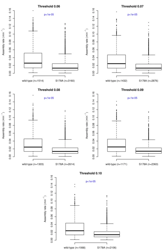
2.13 Modification of FA Detection Threshold and Assembly Rates . . . 32
2.14 Modification of FA Detection Threshold and Disassembly Rates . . . 33
2.15 Modification of Minimum Assembly Phase Length . . . 34
2.16 Modification of Minimum Disassembly Phase Length . . . 35
2.17 Effect of Modifying Sampling Frequency on Wild-type Kinetics . . . 36
2.18 Effect of Modifying Sampling Frequency on S178A Kinetics . . . 37
2.19 Simulation of Static FAs and Properties . . . 38
2.20 Analysis of the Tracking Algorithm Effectiveness . . . 40
2.21 Results of Extracting Phase Length and Rate from Simulated FA Kinetics . . 41
3.1 Determination of Control and Gleevec Treated Cell Movement Direction . . . 49
3.2 Edge and Side FA Processing Methods . . . 50
3.3 Comparison between FA Longevity and Mean Area after Gleevec Treatment . 51 3.4 Arp2/3 Depletion and Cell Speed . . . 55
3.5 Affects of Arp2/3 Depletion on FA Morphology . . . 56
3.6 Arp2/3 Complex Depletion Leads to Poor Global Alignment of Focal Adhesions 59 3.7 Automated Identification of FA Structures . . . 61
3.8 Derivation of Focal Adhesion Alignment Index . . . 64
3.9 FA analysis server overview . . . 67
4.1 Puncta Identification in Single Cells . . . 72
4.2 Properties of Puncta in Control Cells . . . 74
4.3 Determination of ECM Degradation by Puncta . . . 77
4.4 Invadopodia Properties . . . 78
4.5 Cell Identification and Tracking . . . 79
4.6 Quantification of Degradation Amount . . . 80
Chapter 1
Introduction
Visualizating the location of proteins in living cells, through fluorescence microscopy, has become a critical method for investigating the function and activity of individual proteins and protein complexes at the single cell level [1, 2]. The development of these methods and the related advancements in imaging hardware has expanded the type of imaging studies that can be conducted, but has raised problems related to drawing conclusions from the image sets produced. Traditionally, quantitative properties have been extracted manually from cellular biology image sets, but manually analyzing images is time-consuming and prone to potential bias in the selection of which events or structures will be manually assessed. These problems and the continued expansion of imaging assays has encouraged the adaption and development of novel methods to use computer vision methods to automatically assess the results of imag-ing assays. The development and application of computer vision methods to biological images sets is a nascent subfield of Bioinformatics named Bioimage Informatics [3].
1.1 Bioimage Informatics
The analysis of the images resulting from a biological assay shares many components with several closely aligned fields, including Medical Image Processing and Computer Vision [4]. The goals of Medical Image Processing is to develop methods to analyze the results of image collected in a medical context, such as X-Rays or MRIs. While the images analyzed in Medical Image Processing are produced using image modalities drastically different from fluorescence microscopy, many of the same methods are applicable to images produced for a biological experiment. Another overlapping field, Computer Vision, develops methods for teaching computers understanding images. Typically, these images have come from scenes taken using standard cameras, where the set of goals might include identifying the people in the scene and tracking their movements. These type of scenes are very different from the results of fluorescence imaging, but the problems of identifying and tracking objects are shared by both fields. Although Bioimage Informatics, Medical Image Processing and Computer Vision all focus on different goals, the methods developed in for one purpose can often be reused in other fields.
1.1.1 Methods Overview
The methods used in a Bioimage Informatics pipeline vary based on the specific type of images being studied and what type of data needs to be extracted from the images. In general though, each image analysis pipeline must address issues of image registration, segmentation, tracking, data extraction and visualization.
One of the first steps in most image analysis pipelines is registration. The goal of reg-istration is to adjust the raw images collected by the microscope so that the field of view is held constant. In cellular microscopy, registration is often needed to compensate for inexact re-positioning of the objective during multiple field acquisition experiments. In these simple contexts, registration can often be accomplished using translation adjustments and gradient descent. There is also a great deal of overlap in registration methods with other related fields, such as image registration in a Medical Image Processing context [7]. The final result of im-age registration is a set of transformations which can be applied to the raw imim-ages to bring the image set into alignment.
Another stage of a typical Bioimage Informatics pipeline is segmentation. This stage of a typical pipeline analyzes the images and finds all the objects of interest in the image. In fluorescence cellular imaging, the identification of discrete objects of interest is complicated by irregular labeling of the components or low signal-to-noise ratios. Thus, many object segmentation pipelines involve a filtering step where background noise is minimized [8, 9]. After filtering the original images, thresholding selection methods, such as Otsu’s [10] or the unimodal [11], are used to identify potential objects in the image. The resulting set of potential objects may then be matched against a template [9] if the type of object being segmented can be described by a standardized grayscale image. After the segmentation steps have been completed, the result is a list of the pixel locations of each object in the field of view.
sets. One proposed method uses global analysis to optimize the assignment of objects between frames and then uses these inter-frame assignments to build full tracking sequences [13]. Another proposed method uses Kalman filtering to predict the motion of objects moving in a controlled fashion [14]. This type of tracking methodology is most applicable to situations where the biological structure is moving in a very controlled fashion, such as in the case of microtubule tips. All of the proposed tracking methods produce a set of tracks which link the objects segmented in one image of a time-lapse set to another.
Finally, the results of the analysis must be visualized to ensure that the analysis methods have properly identified the structures of interest and new hypotheses can be formed. Sev-eral toolkits and software packages exist for visualizing the raw imaging data or the results of the image processing steps. The visualization toolkit (VTK, www.vtk.org) is an open source package which provides a range of methods for both 2D and 3D visualization. Imaris, pro-duced by Bitplane Software (http://www.bitplane.com/go/products/imaris), is an integrated visualization and quantification system optimized for 3D and 4D image sets. The visualiza-tion steps act as a porvisualiza-tion of an important feedback loop between finding a method to quantify a phenotype of interest and verifying that the phenotype is being property quantified by the analysis system.
1.1.2 High-throughput Image Analysis in Screening
fixed, stained and imaged. The volume of images that result from the screens are impossible to assess manually; image processing methods are necessary to determine the effect of the screen.
One popular open source software for analyzing screening experiments is CellProfiler [5]. This software, originally implemented in MATLAB, but now written in Python, provides a pipeline-based user interface. The user interface presents the most common steps needed to automatically find cells and extract the relevant properties from those cells. The software has been extended to include supervised machine learning methods to automate the learning of cellular phenotypes [16], the ability to analyze the results within the same interface[17] and analyze the images from C. Elegans screens [18].
1.1.3 High-content Image Analysis in Cell Biology
In contrast with high-throughput Bioimage Informatic analysis, high-content image anal-ysis focuses on extracting new properties from biological image assays, typically from time-lapse image sets. These biological experiments are designed to monitor highly dynamic struc-tures, typically in single cells, which are too complicated to be readily quantified via man-ual methods. Although many microscopy heavy field of cell biology have benefited from high-content image analysis, I will highlight the study of cell edge, microtubules and clathrin-coated pits as applications of high-content analysis methods.
One area of cell dynamics that has been extensively quantified using Bioimage Informatics is the cell edge of migrating cells. The edge of migrating cells is highly dynamic with protru-sions and retractions occurring in response to intra- and extra-cellular cues. To quantify the intracellular cues thought to play a role in driving edge movement, a series of biosensors were developed in Klaus Hahn’s lab, including sensors for Rac [24], RhoA [25] and CDC42 [26]. These biosensors allow realtime activity levels of the monitored proteins to be observed using fluorescence microscopy. Early methods of quantifying the biosensor activity levels involved taking line scans radially through the cell edge during specific protrusion or retraction events to quantify RhoA activation during cell edge movement. This line-scan-based method was time-consuming and did not capture the subtleties of cell edge movement. To improve upon these manual analysis methods, Gaudenz Danuser and colleagues developed a set of image analysis methods to automatically determine the local speed of the cell edge [27]. They devel-oped two methods to quantify cell edge movement. The first used the level set method to track the evolution of the cell edge, while the second simpler method used a spring model to fol-low edge movement. The biosensor signals for RhoA, Rac and CDC42 were then correlated with the cell edge movement to determine the proteins order of activation in time and space [28]. By integrating sophisticated imaging methodologies with quantitative image analysis, the relative ordering of intracellular signalling pathways could be dissected in living cells.
high-content image analysis. Microtubules are highly dynamic components of the cytoskeleton which are involved in cellular activities ranging from separating sister chromatids at mitosis to protein trafficking [29, 30]. Microtubules go through cycles of extension and retraction over the course of minutes and are densely packed within the cytoplasm. To analyze microtubule dynamics, fluorescent markers of the growing microtubule tip have been developed and used to observe microtubule development in cells. The density and quantify of tips in cells greatly complicated the process of quantifying the dynamics of these structures. Image analysis meth-ods have been developed to segment, track and analyze the time-lapse images of microtubules [9]. This automated approach provided for a comprehensive characterization of microtubule behavior in living cells and a platform for developing new microtubule quantification metrics. Clathrin-coated pits are another class of cellular structures with complicated dynamics [31]. These structures form on the outer edge of cells and allow cells to internalize extracel-lular factors and recycle the cell membrane. One experimental setup to study clathrin-coated pits labels the developing pit with a ph sensitive dye, allowing hundreds of these structures to be visualized in a single cell. Prior methods for studying these structures used manual track-ing and analysis, but the application of automated segmentation and tracktrack-ing methods allowed the number of quantifiable pits to be greatly expanded [32]. This expansion in the number of quantifiable pits allowed subtle differences in pit lifetime and the effect of an siRNA knock-down of dynamin-2.
1.2 Thesis Contributions
Chapter 2
High-resolution Quantification of Focal Adhesion Dynamics in Living Cells
2.1 Introduction
Focal adhesions (FAs) are dynamic, multi-component protein complexes that serve as points of integration for both mechanical and chemical signaling, while playing a central role in a variety of processes including cancer metastasis, atherosclerosis and wound healing [33, 34, 35]. Characterizing how these structures dynamically change is essential for under-standing cell migration, which requires that adhesions are continuously remodeled as the cell moves forward. During motility, new adhesions are born at the leading edge of a protruding lamellipodia. They then enlarge and are either disassembled at the base of the protrusion in a process known as adhesion turnover, or become longer-lived structures that are eventually dismantled in the retracting tail at the rear of the cell [36, 37, 38]. In this cycle as well as other FA-mediated processes, FA dynamics are highly regulated by structural and signaling molecules [39, 40, 41]. Alterations in the balance of these regulating factors plays a key role in adhesion turnover and thus in adhesion signaling and normal cell function.
the automated detection and characterization of focal adhesions for high-throughput screening studies. For instance, Paran and colleagues [21] have reported on the use of a high-throughput high-resolution imaging system to screen a plant extract library for effects on adhesion mor-phology and distribution. The same high-throughput imaging system was used to perform multicolor analysis on various adhesion components [46] and this system was used in an siRNA screen against adhesion related genes [22]. In these studies, researchers were able to obtain molecular signatures of protein components within focal adhesions, resolve sub-domains within adhesions, and identify clusters of genes that had similar effects on focal adhesion morphology and placement. These studies demonstrate the power of identifying and characterizing large numbers of adhesions within a cell. However, as the approaches used in these studies relied on cell fixation, critical aspects of focal adhesion biology, including their spatiotemporal dynamics, were lost.
Here, we describe a novel system for the quantification of focal adhesion dynamics. This approach utilizes high-resolution (60x oil-immersion) time-series images of living cells gen-erated with TIRF. Image sequences are processed through an analysis system that identifies individual adhesions based on user-defined criteria, tracks their movement through time and collects associated properties concerning their location, shape, size and intensity. As adhesion properties throughout the lifetime of each adhesion are quantified in this approach, a thorough picture of global adhesion spatiotemporal behavior is captured.
Paxillin. Through this analysis we show that the loss of this single phosphorylation site affects adhesion site formation, size and assembly rates. We also verify the broad applicability of the analysis system by also applying the methods to examine time-lapse movies of EGFP-FAK. We are also making the analysis system available under an open source license, to allow the community to use our methods to analyze new experimental systems. These results illustrate the benefit of automated large-scale characterization of adhesion properties and behaviors, allowing both large and subtle differences to be readily detected.
2.2 Results
2.2.1 Quantitative Analysis of Focal Adhesion TIRF Images
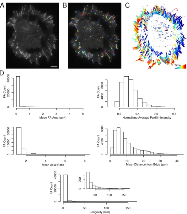
To quantify aspects of focal adhesion spatiotemporal dynamic behavior, we generated an NIH 3T3 fibroblast cell line expressing both EGFP-Paxillin, to label FAs, and a myristoylated-Red Fluorescent Protein (myr-RFP), to identify the cell edge. Cells were plated on fibronectin and imaged with TIRF for 14 hours. We then quantified FA dynamics through a multistage image analysis pipeline (Figure 2.1). Briefly, after high-pass filtering, FAs were identified and segmented with a watershed-based algorithm (see Methods). Characteristics of adhesions identified and quantified at each timepoint included properties such as area, position and flu-orescent Paxillin intensity. Dynamic properties of adhesions, such as velocities and changes in fluorescent intensity, were also determined by tracking and measuring adhesion properties across time steps/images. At each consecutive time step the appearance of new adhesions, called birth events, and the disappearance of adhesions, called death events, were similarly identified and recorded by the software.
of the adhesions in wild-type cells (Figure 2.2D). In general, adhesions are less than 0.2µm2 in size, have axial ratios less than 3 and exist for less than ten minutes, although there are many adhesions that live longer. Both Paxillin fluorescence intensity and the position of the adhesion centroids with respect to the cell edge have skewed distributions. These results demonstrate the capabilities of our system to provide high-resolution and unbiased assessment of FA behavior.
2.2.2 Kinetics of FA Assembly and Disassembly
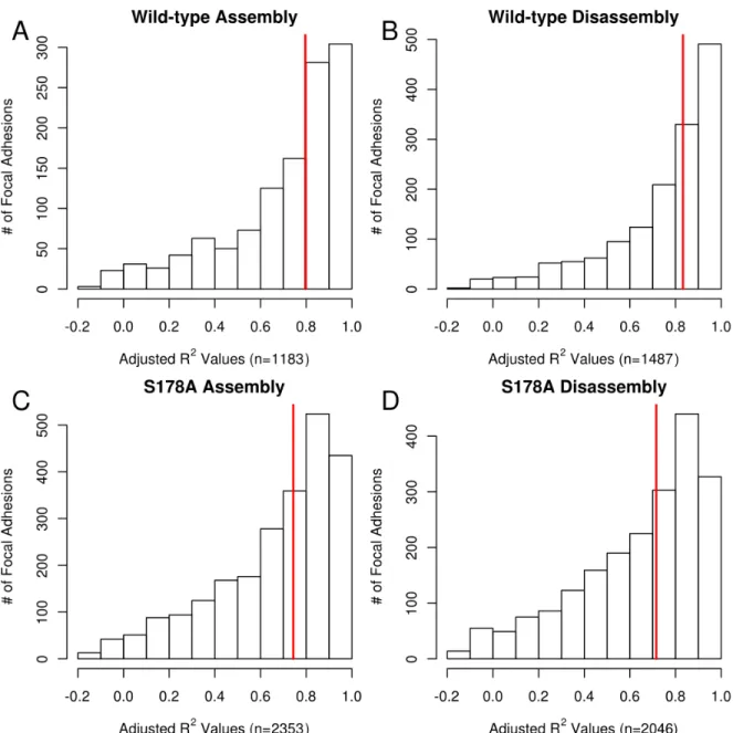
Of particular importance for understanding FA functions is the assessment of adhesion behavior through time. Figure 2.3A-D shows the methods used in determining FA assem-bly and disassemassem-bly rates for individual adhesions. Figure 2.3A depicts an image series of a single adhesion (highlighted in green) from birth, through maturation and stability, and on to death. Using time series information, we quantified the normalized intensity of each adhesion over its lifespan (Figure 2.3B). Readily apparent are the log-linear assembly and disassembly phases, which are automatically fit to a log-linear model (see Methods for details). Our results are consistent with previous work showing that adhesions assemble and disassemble with log-linear progression [39]. Specifically, we found that the log-log-linear fits for most of the adhesions produced R2 values above 0.7 (Figure 2.4). Note that the smaller number of adhesions ana-lyzed relative to Figure 2.2 is due to the need for a minimum adhesion lifetime (>20 minutes) as well as other requirements needed for the accurate quantification of assembly and disas-sembly rates (see Methods). In the example shown in Figure 2.3, a log-linear approximation describes 90.5% and 96.1% of the variance in the rates of intensity increase and decrease, re-spectively (Figure 2.3C, D). In between these two phases we define a stationary/mature phase where intensity remains relatively stable (Figure 2.3B).
minutes, where the detected assembly or disassembly rate is positive and the p-value of the rate model is below 0.05 (Figure 2.3E). The mean rate of assembly of 0.031±0.023 min−1is 55% greater than that of disassembly (0.020±0.014 min−1). While these average rates are slower than earlier published reports, the values determined in previous studies were estimated from far fewer measurements (typically dozens of adhesions) and can be found within the variance of our data set. Thus, this automated computational approach provides a comprehensive pic-ture of the breadth of adhesion assembly and disassembly dynamics without biasing analysis toward any particular subset of adhesions.
2.2.3 Spatial Properties of FA Assembly and Disassembly
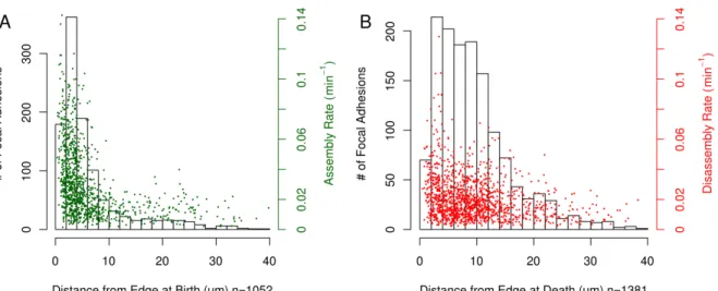
In addition to estimation of assembly and disassembly rates, the analysis pipeline also collects spatial properties of FAs, allowing spatial aspects of FA behavior and dynamics to be similarly studied. Using the same set of experiments used to determine the kinetics of assembly and disassembly, we asked where, relative to the cell edge, adhesions tend to be born/die (Figure 2.5). The majority (63%) of adhesions are born less than 5 µm from the cell edge, with a mean distance from the edge at birth of 6.34µm (Figure 2.5A). In contrast, adhesions tend to die further from the edge with only 27% of adhesions dying within 5µm of the edge (Figure 2.5B). The mean distance from the edge at death was 9.5µm. This suggests the existence of two distinct, but partially overlapping zones within which preferential birth or death of FAs occurs. When looking at both FA birth/death location and assembly/disassembly rate simultaneously, we find that higher assembly rates are observed in births that occur near the edge while no obvious effect of spatial location on the rate of disassembly is apparent (Figure 2.5).
2.2.4 Analysis of EGFP-labeled FAK adhesions
Figure 2.5: Spatial properties of FA positions at birth and death. (A) The majority of adhesions are born within 5 µm of the cell edge and the greatest variance in assembly rates are also observed in this 5 µm band. (B) The distribution of the distance of death location from the cell edge indicates that adhesion disassembly typically occurs along a broader band from the cell edge as compared to the position at adhesion birth. Also, the variance in disassembly rate is roughly the same regardless of the position at adhesion death. This data was collected from 21 EGFP-Paxillin cells.
in NIH 3T3s using TIRFM, we applied the same set of algorithms to determine the assembly and disassembly rate of the FAs. The rates of assembly and disassembly of FAs were found to be statistically indistinguishable when comparing labeled Paxillin to labeled FAK in live cells (Figure 2.6). In contrast, subtle but statistically significant differences in adhesion areas and axial size were found when comparing EGFP-Paxillin vs EGFP-FAK labeled adhesions (Fig-ure 2.7). This result is not unexpected as different spatial and/or stoichiometric relationships are expected for both Paxillin and FAK within FAs [48, 49]. These results further indicate the capability of this system to be generally applicable to the measurement of other adhesion components besides Paxillin.
Paxillin S178A Mutant Perturbation
Figure 2.6: The assembly and disassembly rates of EGFP-Paxillin and EGFP-FAK adhesions are the same. The blue numbers in each plot are the p-values of the difference in median values between the EGFP-Paxillin and EGFP-FAK adhesions. P-values were calculated using the bootstrapped confidence intervals with 50000 replicates. Data from 10 cells are included.
As a proof-of-principle, we utilized our system to investigate the effect of a Paxillin mu-tation (Serine 178 to Alanine) on several aspects of FA behavior. Specifically, a principal regulatory mechanism of Paxillin is phosphorylation, with over 40 sites of phosphorylation currently identified [41]. The roles of many of these phosphorylation sites have yet to be characterized, but many of those that have been studied demonstrate strong effects on cell migration. Of particular interest is the c-Jun N-terminal kinase (JNK) phosphorylation site Serine 178 (S178). Preventing JNK phosphorylation through mutation of this Serine to Ala-nine, or by inhibition of JNK signaling, inhibits cell motility [50, 51]. More recently, it has been shown that phosphorylation of S178 enhances Paxillin’s interaction with FAK, result-ing in tyrosine phosphorylation at residues 31 and 118 [52]. Furthermore, expression of the phosphomimetic Y31D/Y118D Paxillin can rescue the S178A mutant phenotype. This and related work suggests that JNK phosphorylation of Paxillin may be an important early step in adhesion formation. However, the effects of this mutation on adhesion dynamics have not been well characterized.
Using our analysis system we found that the S178A mutation induced a number of sig-nificant effects on the morphological, dynamic and spatial properties of adhesions. The mean area of the S178A mutant adhesions decreased by 23%, while the mean axial ratio decreased by 5% in the S178A mutants (Figure 2.8). Perhaps most relevant to the observed alterations in cell motility, there is an approximately 42% reduction in the median rate of adhesion as-sembly (Figure 2.9A). We also observe a smaller (30%) but statistically significant decrease in median disassembly rate (Figure 2.9B). Thus, the kinetics of FA assembly and disassembly are strongly affected by this mutation, but in a non-symmetric manner.
Figure 2.8: The S178A mutation in Paxillin decreases adhesion size and axial ratio. There are 44685 adhesions in the wild-type and 73305 adhesions in the S178A data sets. The p-values were calculated using the Wilcox Rank Sum test. Data from 9 cells are included in the S178A data set.
occurs) is not dependent and/or sensitive to JNK phosphorylation (Figure 2.6D).
Finally, we compared the length of time spent in the assembly, stationary, and disassembly phases for cells expressing either WT or S178A EGFP-Paxillin. Results suggest that the S178A mutation causes adhesions to be longer-lived, spending a greater amount of time in the assembly phase than WT cells and lesser time in the disassembly phase (Figure 2.10). There is no difference in time spent in the stability phase. As a whole, our results demonstrate the most pronounced effects of the S178A mutation occur in the assembly phase: position at birth, assembly rate, and time spent assembling.
2.3 Methods
2.3.1 Cell Culture
fetal calf serum, 1% L-Glutamine, and 1% penicillin-streptomycin. Fibroblasts were imaged in Ham’s F-12K medium without phenol red (SAFC Biosciences) with 2% fetal bovine serum, 15 mM HEPES, 1% L-Glutamine, and 1% penicillin-streptomycin.
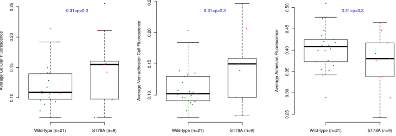
To make stable cell lines, retroviral vectors were transfected into 293 LinXE cells plated in 6 cm dishes with Fugene 6 (Roche) according to the manufacturer’s protocol (using 18µL of Fugene 6 and 4.5µg of DNA). The media was replaced after 12 hours. Viral supernatant was harvested 48 hours after media replacement, passed through a .45µm syringe filter and then added to NIH 3T3s plated at subconfluent densities at a ratio of 1:3 (viral supernatant/normal media). Cells were infected for several rounds until they reached expression levels sufficient for live cell imaging. All of the constructs used in this study have been verified to colocalize with endogenous proteins [50, 53, 54]. No differences were detectable in the expression levels of the EGFP-Paxillin and EGFP-PaxillinS178A constructs (Figure 2.11).
Figure 2.11: There are no significant differences between the expression levels in the EGFP-Paxillin and EGFP-EGFP-PaxillinS178A cell lines. The average intensity of fluorescence inside the cell is shown in three different ways: the overall cell intensity (A), inside the cell not including the adhesions (B) and only the adhesions (C). The error bars are 95% confidence intervals determined using 50,000 bootstrap samples on the mean value.
2.3.2 Microscopy
imaging chamber, complete culture media was replaced with imaging media. Imaging exper-iments for all cells used in this study were conducted within the first 8 hours after plating.
Imaging was performed on an Olympus IX81 motorized inverted microscope equipped with a ZDC focus drift compensator and a TIRFM illuminator, a 60X 1.45 NA PlanApoN TIRFM objective, a cooled digital 12-bit CCD camera (CoolSnap, Roper Scientific), a 100 W Mercury arc lamp, and MetaMorph imaging software. The 488 nm laser line from a Krypton-Argon ion laser (Series 43, Omnichrome) was controlled with a custom laser launch/AOTF (LSM Technologies). Imaging of the cells expressing EGFP-FAK was performed on a Nikon Eclipse Ti inverted microscope equipped with the Perfect Focus System, a TIRF illuminator, a 60X 1.45NA PlanApoN TIRF objective, a a cooled digital 16-bit EMCCD camera (Quan-tEM: 512SC, Photometrics), an Argon ion laser (Melles Griot) controlled with a custom laser launch/AOTF, and Nikon Elements imaging software. Images were acquired with 22 binning, except for images of EGFP-FAK expressing cells, which were acquired with 11 binning. Im-ages were gathered once every minute. Illumination intensity was controlled with either the AOTF (TIRF excitation) or neutral density filters (epifluorescence excitation). Simultane-ous TIRF images of EGFP and epifluorescence images of RFP were acquired using an 80/20 (TIRF/Epifluorescence) splitter mirror, a custom dichroic mirror (Chroma) and the following band-pass filters: EGFP (HQ 525/50); RFP (HQ580/30, HQ 630/40). In total, 21 EGFP-Paxillin, 9 EGFP-PaxillinS178A and 10 EGFP-FAK cells were included in this study. The EGFP-Paxillin experiments were conducted over four days, while the EGFP-PaxillinS178A experiments were conducted over three days and the EGFP-FAK experiments were conducted over three days.
2.3.3 Image Processing
by an empirically determined value set to identify adhesion pixels. The water segmentation method was used as described, but with the following modifications. When a pixel acts as bridge between two large adhesions, where large is defined as 40 or more pixels (1.85 m2), the bridge pixel is assigned to the adhesion whose centroid is closest to the bridge pixel. Also, holes in any single adhesion were filled using the same water segmentation algorithm. Be-tween 200 and 600 adhesions were found in each image from the experimental data. The average signal-to-noise ratio was 6.04 as calculated by dividing the mean of the adhesion intensity by the standard deviation of the backgound pixels [55]. After each focal adhesion has been identified, characteristic adhesion properties, such as those in Figure 2, are then collected.
Cell edges were found by analyzing the myr-RFP images using a method similar to that described in a prior publication [27]. This method automatically identifies a single threshold which splits the myr-RFP images into cell body and background regions. Briefly, a histogram of all the intensity values for a single image was collected and split into 1000 equal sized bins. The counts of each bin were then smoothed with the loess algorithm (Polynomial order 2, 5% of data included in each fit). This smoothed histogram has two peaks corresponding to the background region and the cell body. The local minima and maxima in the smoothed histogram are found and the two maxima at the lowest pixel intensity bins identified. The threshold for image segmentation is set to the minima between the set of maxima found in the prior step. After thresholding the image, the connected regions are identified and the regions less than 10 pixels in area are discarded. The cell edge is defined by the border pixels of the connected regions.
2.3.4 FA Tracking
each sequential image a FA can either be born, continue into the next time step, merge or die. The birth-death-merge processes are detected by examining the properties extracted from the segmented adhesions. The results of this tracking algorithm are assignments of the FAs identified in each image into lineages that track the development of the FAs during the course of the experiment.
Figure 2.12: Flow chart for the tracking software adhesion following algorithm.
in the following image, the FA closest to that adhesion in terms of the Euclidean distance between each adhesion’s centroid is assigned as a match. Adhesions in the next frame that are not selected via either of these methods, but still overlap with an adhesion in the current frame are marked as being created via a split birth event. Adhesion births that are the result of split events are dealt with in later filtering steps. All of the living focal adhesions are assigned a corresponding FA in the following image by these percentage overlap and centroid distance rules.
This process of assigning live adhesions in one frame to corresponding adhesions in the following frame produces sets of adhesions that are predicted to merge. Some of these merge events are true merge events where one adhesion has joined with another, while others are adhesions which die, but are erroneously assigned as merge events. When a FA does not overlap with the FA it is predicted to become, this FA is assumed to have died and its lineage is ended. These adhesions are also marked as having undergone a death, which will be used in later filtering steps. For the remaining merge events where more than one adhesion has been predicted to merge in the next frame, one of the merging FA lineages is selected to continue, while the other FA lineage is predicted to end. When the adhesions predicted to merge differ in size by at least 10%, the larger adhesion’s lineage is continued. If the merging FA’s sizes do not differ by at least 10%, the lineage whose current centroid is closer to the adhesion centroid in the following image is predicted to continue. By this sequence of rules, each merge event is resolved so that corresponding FAs in experimental data images are determined.
cells. The differences in the average number of adhesions are due to longer experiments in the EGFP-PaxillinS178A and EGFP-FAK data sets.
2.3.5 Calculating Assembly and Disassembly Rates
With the adhesions tracked through each experiment, the characteristic properties deter-mined for each adhesion in each frame of the time-lapse movie are collected into a set of data time series representing the properties of each adhesion through time. One type of time series follows the mean intensity of Paxillin through time, making it possible to estimate the rates of assembly and disassembly of Paxillin for each adhesion. An automated method to estimate the rates of assembly and disassembly was developed. This program automatically fits linear models to the log-transformed time series of Paxillin intensity values for both the assembly and disassembly phases of the FA life cycle.
A log-linear fitting method was adapted and extended to allow for the automated deter-mination of assembly and disassembly phase lengths [39]. Briefly, log-linear models are fit to all the possible assembly and disassembly phases greater than or equal to a user specified minimum length. The assembly phase is assumed to occur at the beginning of the time series, whereas the disassembly phase is assumed to end with the last point in the time series. Each of the fits collected were normalized by either the first (assembly rate calculations) or last point (disassembly rate calculations) in the time series and log-transformed, as described [39].
2.3.6 Results Filtering
Several filters are used to analyze the data sets collected with these analysis methods. When determining the assembly and disassembly rates, only adhesions with at least 20 Pax-illin intensity time points were analyzed. This ensured that there was sufficient data available to correctly detect the assembly and disassembly rates. Adhesions whose birth was the result of a split event with another adhesion were also excluded from the assembly rate calculations, while adhesions whose lineage ended with a merge event were excluded from the disassem-bly rate calculation. Assemdisassem-bly and disassemdisassem-bly fits whose linear model p-values were above 0.05, indicating that the slope of the linear model was not significantly different from zero, were also excluded from the data set.
A separate set of filters was used to determine the length of each phase (assembly, stability and disassembly) in the adhesion intensity time series data. In order to estimate the length of time an adhesion spends in the stability phase, we required that both the assembly and disassembly phases be observed. In addition, the adhesion birth could not have been the result of a split event and the death of the adhesion not the result of a merge. The filter also excluded those adhesions where the p-value of either the assembly or disassembly linear model was greater than 0.05.
2.3.7 Parameter Testing
(Figure 2.15 and Figure 2.16). Finally, we tested the results of changing the image sampling rate by discarding every other collected image in the same set of experiments (Figure 2.17). Discarding half of the images did not significantly affect the assembly or disassembly rates, but did have a slight effect on the distribution of the adjusted R2 values (Figure 2.18). From these parameter testing examples, we concluded that selection of a single set of parameters as determined by the user, provided a robust description for any of the differences between cell lines in terms of assembly and disassembly rates.
2.3.8 Software Testing
In order to test the baseline performance of the algorithms, a set of gold standard images were produced with sets of FAs having specific, predefined properties. In general, validation tests consisted of simulating a time-lapse microscope field of view that mimicked the observed properties of the adhesions (Figure 2.19A). Since our results are consistent with prior findings based on manual methods of adhesion identification, the simulated range of properties was set to be similar to those observed in the experimental data. For all simulated experiments, a Gaussian noise model (mean 0, variance of 2*103) was used as a background to simulate the cell environment. These parameters were chosen as they produced distributions of short-lived adhesions that were empirically similar to those observed experimentally. Also, all simulated adhesions were circular and the same background noise model was used to perturb intensities assigned by the software to each simulated adhesion.
level were readily detected with both the predicted intensities and sizes (Figure 2.19).
The moving simulation was designed to probe the tracking algorithm’s performance in following adhesions of various sizes and intensities. The simulation consisted of sliding the adhesions across the field of view at different rates (Figure 2.20A). As expected, the smaller adhesions were more difficult to track, with a nearly linear relationship between the ability to track an adhesion moving at a certain rate and its corresponding radius (Figure 2.20B). As long as the adhesion is detectable, there does not appear to be any differences in the intensity versus tracking accuracy (data not shown).
To conduct the adhesion kinetics tests, sets of adhesions were simulated that went through logarithmic assembly and disassembly phases. The assembly and disassembly rates were varied by shortening or lengthening the amount of time each adhesion spent reaching its max-imum intensity. The stability period in each of these adhesions was set to five frames. Assem-bly and disassemAssem-bly lengths between 10 and 20 were all tested. In order to avoid biasing the automated assembly and disassembly phase fitting software to higher phase lengths, the mini-mum phase length was set to five time points during image analysis. Overall, the software was able to reliably extract both the expected assembly and disassembly rates and length of time spent in each phase (Figure 2.21). There were several samples in the longer phase lengths that were predicted to have substantially shorter assembly and disassembly phase lengths than that specified by the software, but these simulated adhesions were in the minority and did not sig-nificantly affect the confidence intervals around the mean assembly and disassembly lengths. These simulations further support the accuracy of results derived from applying the same sets of algorithms to the analysis of adhesions in living cells.
2.3.9 Statistical Tests
or median distribution. From these distributions the p-value was determined using the per-centile method. The bootstrap method was too computationally intense to compare datasets, such as the area and axial ratio of the adhesions, with significantly more points than 2000 data points. Instead, the Wilcox Rank Sum test was used to find the p-value in these cases.
2.3.10 Software Availability
The most recent version of the software system is available from the Gomez lab website (http://gomezlab.bme.unc.edu/tools). In addition to the source code, released under the BSD license, there is a sample movie that can be used to test the success of installing the analysis system. The software has been tested on Mac OS10.5 and Ubuntu Linux 10.04.
2.4 Discussion
We have described the development of a set of computational tools suitable for the global characterization of FA spatiotemporal dynamics and assessing the results of network pertur-bation on adhesion properties and behavior. The S178A mutation was presented as a proof-of-concept perturbation study for the application of these tools to the analysis of complex FA phenotypes. Through this analysis, we were able to show that adhesion dynamics fall into dis-tinct behavioral subtypes occurring in different regions of the cell, and that the S178A Paxillin mutant causes significant changes in FA assembly and disassembly. While requiring further investigation, these observations suggest a potential mechanism for the previously observed migration defects [50] and suggest that JNK, via Paxillin, may play a significant role in the control of the FA lifecycle.
conditions (see Figure 2.19, Figure 2.20, Figure 2.21 and methods). The differences detected between the wild-type and S178A mutants are robust, being preserved through a range of pa-rameter choices for the adhesion detection limit and the minimum length of the assembly and disassembly phases. The rate at which images were taken in this work (1 sample/min) also ap-pears to be over the sampling rate needed to accurately measure the assembly and disassembly rates of long-lived adhesions (Figure 2.17 and Figure 2.18).
Our analysis system integrates methods for automatically identifying and extracting rates of FA assembly and disassembly. We find that the assembly and disassembly rates detected using these automated methods encompass the rates determined using manual methods [39], while quantifying vastly greater numbers of adhesions. We also find that adhesions labeled with an alternate adhesion marker, FAK, also allows a similar number of adhesions to be quantified and that these adhesions are similar to those detected using fluorescently labeled Paxillin. Differences in the mean rates detected by manual versus automated searches can be attributed to several factors. First, the rates determined using manual methods originate from user-specified adhesions of interest. Such adhesions may be chosen based on specific local-ization properties, such as selecting only those adhesions found within particular cell regions, while the presented results do not make any distinction between adhesions present in different cellular structures a priori (though the properties of adhesions at particular locations can be determined a posteriori). In addition, due to our emphasis on observing the birth, death and taking multiple samples during the assembly and disassembly phase of an individual adhesion, our rate analysis focused on long-lived adhesions, which might have different properties than those measured in studies encompassing primarily short-lived adhesions. Finally, as our soft-ware analyzes all adhesions regardless of the brightness of the adhesion, we avoid biases that may occur through, for example, preferential selection for analysis of large or highly visible adhesions. Thus, the automated methods described here greatly extend the types of adhesions that can be readily analyzed, as well as the range of properties that can be quantified.
assembly and disassembly events are most concentrated. These assembly and disassembly regions overlap, but remain distinct. The greatest concentration of assembly events occurs within 5µm of the cell edge. Previous studies in the same cell line indicate that this 5 µm range coincides with the end of the lamellipodia and the beginning of the lamella, where the structure of the actin cytoskeletal network changes significantly. Recently published data indicate that this transition, where stable actin structures differentiate into branched structures that exert force on the leading edge for protrusion, is determined by interactions between the cytoskeleton and adhesion proteins [56]. Further investigation will be required to more fully interpret this observation and its relation to the lamella-lamellipodium interface [57].
Figure 2.22: Summary of results and conceptual model of how the S178A mutant affects the adhesion life cycle. Durations and slopes are shown to scale.
also measured decreases in adhesion size [22].
Chapter 3
Extensions to Focal Adhesion Analysis
The framework developed in Chapter 2 makes it possible to identify, track and quantify FA structures in living cells. These methods have provided a foundation for the development of new methods to quantify the global structure of FA organization. The FA analysis tools have been expanded through two additional projects. The first project was developed in col-laboration with Zaozao Chen to identify FA structures near the cell edge without the use of a secondary marker as was used in Chapter 2 (see Section 3.1). This project also required the development of an automated method to determine the direction of cell motion without a secondary cell edge marker. The second project was developed in collaboration with James Bear’s laboratory to quantify the effects of Arp 2/3 knockdown on FA (see Section 3.2). For each of these projects, I will give a brief overview of the relevant biological background and then describe the methods and results.
3.1 Detection of Edge Adhesions and Cell Movement Direction
3.1.1 Introduction
The study of cell migration is essential for understanding a variety of processes, including wound repair, the immune response and tissue homeostasis; importantly, aberrant cell migra-tion can result in various pathologies [35, 58]. However, the relamigra-tionship between cytoskeletal dynamics, including actin network growth, contractility, and adhesion, and cell shape and migration is not fully understood.
Abl family tyrosine kinases are ubiquitous non-receptor tyrosine kinases (NRTKs) in-volved in signal transduction [59, 60, 61]. They can interact with other cellular components through multiple functional domains for filamentous and globular actin binding as well as through binding phosphorylated tyrosines (SH2), polyproline rich regions (SH3), DNA (Abl), and microtubules (Abl Related Gene (Arg)) [62, 63]. Abl family tyrosine kinases have also been found to regulate cell migration [63, 64]. In some cases, Abl family kinases have been reported to promote actin polymerization and migration [65] as well as filopodia formation during cell spreading [66, 67]. By contrast, in other studies, Abl was found to restrain lamel-lipodia extension [68, 69] or inhibit initial cell attachment to the substrate [70]. Abl family kinases have been suggested to regulate cell adhesion size and stress fiber formation [71]; Li and Pendergast recently reported that the Abl family member Arg, could disrupt CrkII-C3G complex formation to reduceβ1-integrin related adhesion formation [72]. Thus, a complete understanding of how Abl family kinases regulate cell migration is lacking [63, 64].
and control cells required comparisons to be made between adhesions at the leading edge, side and back portions of the cell. Since these cells would not tolerate the addition of a sec-ondary membrane-associated fluorescent marker, new methods were developed and applied to automating the identification of adhesions in these regions.
3.1.2 Methods
To detect the cell movement direction without a cell mask signal, the location of the de-tected adhesions was used as a proxy. First the centroid position of each adhesion was found in each image of the time-lapse set. Then, the x and y components of the single FA centroid values were averaged, giving the adhesion centroid position. Finally, the direction and magni-tude of the adhesion centroid movement was calculated between each frame of the movie and averaged over the course of the experiment to determine the overall direction of cell motion. To test the results, movement vectors were determined by hand for each set of images and compared to the automatically determined direction (Figure 3.1). There was good agreement between the automatically determined and manual direction results. This method was effec-tive for the movies partially because none of the sample cells changed direction during the course of the time-lapse. If this were to occur, a more complicated method of combining the between frame movement direction vectors would need to be developed.
With the direction of cell movement determined, I then used the convex hull containing the identified adhesions as a surrogate for the cell edge. The adhesions in the NBTII cells used in this study generally lined the entire border of the cell, making the convex hull a good surrogate for the cell edge (Figure 3.2A). The distance from the centroid of each adhesion to the convex hull cell edge was calculated (Figure 3.2C).
Figure 3.1: Comparison between direction of cell motion calculated manually (By Hand An-gle) and automatic (Adhesion Centroid AnAn-gle) methods in control (A, n=9 time-lapse experi-ments) and Gleevec-treated (B, n=8 time-lapse experiexperi-ments) cells.
was calculated (Figure 3.2B). This angle was near zero for adhesions close to the leading edge and became larger as the adhesion was located on the side or back of the cell. After tracking the adhesions through the rest of the movie, the average value of the convex hull distance and the angle formed with the direction of motion was determined and used to classify each adhesion as either leading, side or central/trailing (Figure 3.2D). Finally, a visualization was produced that indicates the classification of each adhesion (Figure 3.2E).
Figure 3.2: Focal Adhesion Identification and Classification Methods. (A) Sample frame from a time-lapse image sequence of EGFP-Paxillin in a Gleevec treated cell. The adhesions iden-tified are outlined in yellow. (B) The filtering results applied to identify the leading cone of adhesions. The blue lines mark the region from -80 degrees to 80 degrees of the cell move-ment direction with the intersection of the two lines at the adhesion centroid. The adhesions highlighted in green are those whose average angle falls in the -80 to 80 degree threshold, while the red highlighted adhesions fall outside those cutoffs. (C) The results of filtering ap-plied to identify adhesions near the convex hull edge. The convex hull is indicated in purple. The green adhesions are those within the 40th percentile of all average adhesion distances, while the red indicates adhesions outside the 40th percentile. (D) The distribution of adhesion angle and distance, with the corresponding classification of each adhesion in the image set. (E) Adhesions are highlighted according to the same color scheme as in part (D).
3.1.3 Results
average area increased by 40%, while the area only increased by 29% and 16% on the side and trailing/central adhesions, respectively. These proof-of-concept results demonstrate the utility of subdividing adhesions into classes based on their location.
3.2 Development of Global Methods for Adhesion Direction Quantification
3.2.1 Introduction
For a cell to move in a directed fashion, it must be able to detect a difference in the external environment. The study of how cells detect the outside environment and then move in a coordinated fashion is divided into several sub-fields depending on the type of signal being detected. If the cell uses a soluble chemical factor, the migration is called chemotaxis. If the cell uses a factor attached to the surface over which the cell is migrating, then the migration is called haptotaxis. Finally, if the cell uses the mechanical properties of the substrate, such as stiffness, to determine where to migrate, the migration is called durotaxis. Understanding how eukaryotic cells sense these directional cues and respond with directed movement remains one of the central problems of modern biology.
Chemotaxis is perhaps the most well understood form of directional motility and involves a variety of signaling pathways connecting cell surface receptors to the motility machinery inside of cells [73]. Based mainly on studies of rapidly migrating amoeboid cells such as neutrophils and Dictyostelium cells, these signaling cascades are thought to trigger directional protrusions at the leading edge by controlling actin assembly pathways [74]. Haptotaxis and durotaxis are much more poorly understood but likely involve signaling events triggered by adhesive receptors such as integrins [75].
proteins and subsequent clustering lead to the formation of nascent focal complexes appear-ing continuously at the distal margin of the lamellipodium. A subset of the focal complexes mature into focal adhesions that are connected to bundled actin stress fibers.
The central pillar of the actin network found in lamellipodia is the seven-subunit Arp2/3 complex. The structure, regulation, and biochemical properties of this complex have been ex-tensively studied in vitro (reviewed in [79]). Once activated by nucleation-promoting factors (such as SCAR/WAVE), Arp2/3 nucleates actin daughter filaments as branches off of existing mother filaments. The localization of Arp2/3 to actin filament branches in vivo [80, 77] and the functional role of this complex in lamellipodia formation in cells has been confirmed by many [81, 82, 83], but not all studies [84]. Recently, the existence of actin branches in lamellipodia has been called into question by experiments using alternate electron microscopy techniques [85].
Functional studies of Arp2/3 in vivo have been severely hampered by effects on viability observed upon loss of this complex in a variety of organisms. Genetic deletion of Arp2/3 subunits is lethal in yeast and Dictyostelium, and mouse knockouts produce preimplantation lethality [86, 87, 88]. These data led to the prevailing notion that the Arp2/3 complex is essential for viability in eukaryotes [89].
In this work, it was demonstrated that Arp2/3 is not strictly needed for eukaryotic cell viability. In mouse cells lacking the Ink4A and Arf genes, a nearly complete knockdown of Arp2/3 is possible. For the knockdown to be stable, it was necessary to target two components of the seven subunit Arp2/3 complex simultaneously. Throughout the rest of this section, the Arp2/3 knockdown cell line will be referred to as 2xKD. In addition to the knockdown of Arp2/3, a recently developed small molecule inhibitor of Arp2/3 (known as CK-666 and an inactive analog CK-686 [90]) was used to confirm the effects of the knockdown.
siRNA vector) cells were plated on differing concentrations of ECM components, and motility speed was measured. The results of these experiments appear in the Results section. To test the chemotactic response of the 2xKD cells, a microfluidic chamber was designed, which made it possible to create uniform quantitative gradients of Plalet-derived growth factor (PDGF). Both the 2xKD and NS cells migrated towards the PDGF source, indicating that Arp2/3 is dispensable for chemotaxis. Using the same microfluidic chamber, the haptotactic response of the 2xKD cells was tested using gradients of firbronectin, laminin, and vitronectin. Using each of these ECM components, the 2xKD cells were unable to detect the ECM component gradient, whereas the NS cells could detect and migrate up the ECM gradient. These disparate results in chemotactic and haptotactic responses inspired examination of the FAs in the 2xKD and NS cells under varying concentrations of fibronectin.
3.2.2 Results
Depletion of the Arp2/3 Complex Eliminates Cell Speed Response to Changes in ECM
Concen-tration
Figure 3.4: Arp2/3 Complex-Depleted Cells Cannot Respond to Concentration Changes in Extracellular Matrix(A) Single-cell speed of NS and 2xKD cells plated on different concen-trations of fibronectin was plotted (N>30). Error bars represent 95% confidence intervals.
Depletion of the Arp2/3 Complex Leads to Altered Focal Adhesion Morphology and Dynamics
alternative pathways of adhesion assembly.
Figure 3.5: Depletion of Arp2/3 Complex Leads to Defective Focal Adhesion Morphology and Dynamics (A) Mixed NS (expressing GFP) and 2xKD cells (marked by red asterisks) were immunostained for endogenous Paxillin (Pax), focal adhesion kinase (FAK), Vinculin (Vin), and F-actin. Scale bar, 10µm. (B) Representative time-lapse TIRF images of an NS cell expressing GFP-Pax and LifeAct-tagRFP. (C) Representative time-lapse TIRF images of a 2xKD cell expressing GFP-Pax and LifeAct-tagRFP. (D) Table of focal adhesion param-eters: NS versus 2xKD plated on 1, 10, and 100 µg/ml FN; Rat2 fibroblasts treated with CK-666 or CK-689 on 100µg/ml FN. Numbers after the±indicate 95% confidence intervals as determined by a t-distribution fit. See also Figure 3.7.
and 2xKD cells across three concentrations of fibronectin (Figure3.5D). With increasing fi-bronectin concentration, mean focal adhesion area and mean longevity were increased in the NS cells. Interestingly, neither of these properties varied significantly in the 2xKD cells as a function of fibronectin concentration. Mean long axis length and mean axial ratio were the same in both cell types and did not vary with fibronectin concentration. The number of adhe-sions per cell (per 10 min) trends in the opposite direction in NS and 2xKD cells as a function of fibronectin concentration. Control NS cells had decreased numbers of adhesions per cell with increasing fibronectin, whereas Arp2/3-depleted 2xKD cells had increased numbers of adhesions with increasing fibronectin concentration. We also examined the focal adhesions in Rat2 fibroblasts expressing GFP-Paxillin treated with the Arp2/3 inhibitor CK-666 or its inactive analog CK-689. With transient Arp2/3 inhibition, some of the same trends in focal adhesion properties were evident (and statistically significant), but these trends were much less pronounced than with RNAi-based depletion. Together these data indicate that some fo-cal adhesion properties are unchanged by Arp2/3 depletion, whereas others are altered when Arp2/3 is depleted.
Lamellipodia Promote Global Focal Adhesion Alignment
To quantify global focal adhesion alignment, we developed a method to measure the devi-ation of adhesion angles from the most frequent or dominant angle observed in the whole cell (see Figure 3.8 and next section). To reliably determine the angle of the individual adhesions, we limited our measurements to those adhesions with a length/width ratio of at least 3 (Fig-ure 3.6B). By plotting the angles of all the adhesions that met this criterion, we were able to determine the most frequent or dominant focal adhesion angle by rotating the image frame of reference until the standard deviation (SD) was minimized and the peak of the distribution of angles moved close to zero (Figure 3.8B). The dominant focal adhesion angle was simply the degree to which the image had to be rotated to center the peak over zero. The Focal Adhe-sion Alignment Index (FAAI) is directly related to the standard deviation of this distribution; F AAI = 90−SDin order to have a higher index value correspond to more aligned adhesions (Figure 3.6C). To illustrate this measurement, a cell with high FAAI and low FAAI are shown in Figure 3.6D.
Using this metric, we quantified the FAAI of NS and 2xKD cells plated on 1, 10, and 100 µg/ml fibronectin. We observed increased alignment of adhesions across the cell (increasing
FAAI) with increasing fibronectin concentration in the NS cells, whereas the alignment in the 2xKD cells was decreased compared to the NS cells and was constant at all fibronectin con-centrations (Figure 3.6E). Because mean adhesion area showed similar trends (Figure 3.5D), we tested whether focal adhesion alignment was independent from adhesion area. To do this, we recalculated the FAAI considering only small, medium or large adhesions in the NS and 2xKD cells (Figure 3.6F). Regardless of which size adhesions we used to calculate FAAI, the same difference in alignment was observed between NS and 2xKD cells. To ensure that this result was not specific to the expression of GFP-Pax, we calculated the FAAI of NS and 2xKD cells expressing fluorescent fusions of FAK and Vinculin. With all three markers, 2xKD cells showed significantly lower FAAI compared to NS control cells (Figure 3.6G). Finally, we confirmed this result in Rat2 fibroblasts treated with the Arp2/3 complex inhibitor CK-666 and we observed decreased FAAI with Arp2/3 inhibition (Figure 3.6H). These results suggest that one of the principal functions of the lamellipodium is to promote global focal adhesion alignment.
3.2.3 Methods
Calculating the Focal Adhesion Alignment Index
properties (mean area, axial ratio, major axis length, minor access length and longevity) were only calculated for adhesions where both a birth and death event was detected.
Figure 3.7: Automated Identification of Focal Adhesions. (A) TIRF image of an NS cell expressing GFP-Pax on a 100 g/ml FN-coated surface (bar = 10 µm). (B) High-pass filter applied to the image in part A. (C) Distribution of high-pass pixel intensities from the entire time-lapse image series in part A. The red dotted line indicates the focal adhesion pixel rejec-tion threshold of the mean plus two standard deviarejec-tions. (D) Locarejec-tions of focal adhesions as determined by applying the threshold determined in part C to the high-pass filtered image in part B and overlaying the result on the image in part A. Each identified adhesion is outlined in yellow.
the focal adhesion alignment index (FAAI, Figures 3.8A and 3.8B). The index is determined by a two-step process. The first step involves collecting and filtering the adhesion angles in each image of the time-lapse, while the second step involves searching for a reference angle that minimizes the deviation between all of the adhesion angle measurements. We began the first step by segmenting the adhesions from each frame of a time-lapse movie. From this set of identified adhesions in each frame, we calculated the best-fit ellipse to each adhesion (Figure 3.8A). From this ellipse, we found the length of the major axis, the length of the minor axis and the angle the major axis of the adhesion made with the positive x axis. Angle measurement was on a scale of 90-90 to avoid the ambiguity of the 360 measurement scale (Figure 3.8A). We set the minimum ratio of the lengths of the major over minor axes to 3 as a filter to select adhesions whose orientation could be determined (Figure 3.8A). After collecting the adhesion angles with the positive x axis as the reference, the second step of calculating the index began with a search through a range of potential reference angles. The search began with the x axis as the 0 position and the calculation of the standard deviation of the adhesion angles (Figure 3.8B column 1). Then, the reference angle is increased by 0.1, the adhesion angles with the new reference axis are recalculated, and the standard deviation is measured. This search process continued until the full range (0-179.9) of potential reference angles had been sampled (see intermediate reference angles in Figure3.8B columns 2-4). The FAAI is calculated for all reference angles as follows: FAAI=90-SD(adhesion angles at a given reference angle).
list of angles that maximize the FAAI as the dominant angle. The final number reported is the value of the FAAI at the dominant angle.
We also wanted to measure the variation through time in the angles formed by single adhesions. To measure single adhesion angle variation, we tracked the adhesions identified through each frame of the movie. From this data set of tracked adhesions, we excluded angle measurements with a major/minor length ratio less than 3 and determined each adhesion’s dominant angle. We rotated each adhesion’s frame of reference to match that adhesion’s dominant angle and measured the mean absolute value difference between the adhesion’s first measured angle and the rest of the adhesion’s angle measurements.
3.2.4 Discussion
In this work, we have established a stable Arp2/3-depleted cell line that allowed us to study random and directional cell motility in the absence of lamellipodia. The depletion of the Arp2/3 complex causes striking changes in cell morphology, motility, and global focal adhesion geometry.
Spatial Organization of Cell-Matrix Adhesions and Global Cell Motility
Although focal adhesions have been intensively studied for decades, the processes that spatially organize these structures in an ensemble manner across the whole cell are poorly understood. Our results indicate that lamellipodia play a major role in bringing spatial coher-ence to focal adhesion formation. Without lamellipodia, focal adhesions are poorly aligned with each other, which may explain why these cells migrate slowly. An open question is how lamellipodia promote the alignment of focal adhesions. One possibility is that the retrograde