A Clustering Heuristic Algorithm for Scheduling Periodic and Deterministic
Tasks on a Multiprocessor System
Muhammad U. Ilyas and Shoab A. Khan
Communications Enabling Technologies/ Avaz Networks
5-A, Software Technology Park, Constitution Avenue, F-5,
Islamabad – 44000, Pakistan.
E-mail: [email protected]
Abstract
In this paper, a Clustering Heuristic Scheduling Algorithm (CHSA) for periodic and deterministic tasks on a multiprocessor system is presented. It is assumed that system repeatedly processes scheduled tasks periodically. The system consists of an array of independent processing elements and no inter-processor communication overheads. The system may or may not require code fetches for the execution of different tasks. The CHSA receives different tasks with a variable probability distribution over time. The CHSA attempts to increase the average processor utilization of the system, reduce the code fetch time overhead by attempting to cluster similar tasks and reduces power consumption across the system by attempting to keep as many processors as possible unutilized, thereby allowing them to be kept in a low-power mode.
Keywords - Scheduling; scheduling heuristic; clustering; multiprocessor systems; periodic tasks; deterministic tasks.
1. Introduction
This paper is focused towards a scheduling heuristic algorithm that attempts to schedule i periodic tasks with soft deadlines on a multi-processor system. The algorithm has been designed for a linear array of P processing elements. Each processor has a program and data memory.
All tasks have a time period T. All tasks are non-resident. Non-resident tasks are tasks whose code has to be loaded from an external source. The system loads data and code using a memory interface. The memory interface is the bandwidth bottleneck of the system. It is assumed that code fetch times are significantly higher than data fetch times. Therefore, the scheduler attempts to reduce repeated code fetches caused by scheduling dissimilar tasks on the same processor.
A processor’s program memory is big enough to store code of only one task at a time. The time period P is divided into S time slots. The scheduler is invoked at the start of each time slot t as an ISR, i.e. all scheduling decisions have to be taken at the start of a time slot.
The CHSA consists of a Processor Selection Algorithm (PSA), a Time-slot Selection Algorithm (TSA) and a System Utilization Controller (SUC). The PSA assigns parameters to each processor according to the nature of the task that is to be scheduled. It then prioritizes the processors capable of processing the new task according to each processor’s status parameters. The PSA returns a list of processors, in order of preference, which it passes to the TSA. The TSA then attempts to assign the task to a time-slot on a processor beginning with the processor assigned the highest priority. For that purpose the TSA creates a simplified Gantt chart in the form of a link list from the schedule it maintains for each processor. The TSA then searches the link list for different patterns in their order of priority. The SUC limits the number of tasks allowed to be scheduled on the system in order to keep the ratio between the code fetch requests and data fetch requests within acceptable limits. The CHSA was successfully tested with a simulator of a multiprocessor system.
2. Processor Selection Algorithm
The CSHA has to make two decisions when scheduling a new channel. The first decision selects the processor on which the new channel is scheduled. This is done by the Processor Selection Algorithm (PSA). The second decision selects the time slot(s) in which the new task is scheduled and processed on the selected processor.
2.1. Processor Prioritization
The CSHA reads the idle time for all processors from the status information it maintains. It creates a list of all those processors whose idle time is greater or equal to the processing time required by the new task. This way the CSHA generates an unsorted list of processors with the
available resources to process the new channel. The processor status table maintains how many channels of each task are scheduled on each processor separately. This information is used to generate the values for three temporary data objects. These are
BOOL thisTask; BOOL otherTasks; INT otherTasksCount;
These values of these objects are updated every time a new channel is scheduled.
thisTask: This flag is set if at least tasks of type THIS are
already scheduled on that particular processor.
otherTasks: This flag is set if tasks of types other than
THIS are scheduled on that particular processor.
otherTasksCount: This counter maintains the number of
types of tasks other than THIS that are scheduled on that particular processor.
Based on the values we obtain for each processor we now select the processor. The order of preference for selecting a processor according to these three values is given below. The term THIS task refers to the task type the scheduler is attempting to schedule at the moment. 1. Processor dedicated to THIS type of tasks.
thisTask == TRUE otherTasks == FALSE otherTasksCount == 0 2. Free Processor. thisTask == FALSE otherTasks == FALSE otherTasksCount == 0
3. Processor running THIS task along with tasks of other types.
thisTask == TRUE othertTasks == TRUE otherTasksCount == min.
4. Processor running only tasks of other types.
thisTask == FALSE otherTasks == TRUE otherTasksCount == min.
Processors with equal priorities are arranged in descending or ascending order of their respective processor ID numbers.
3. Time-slot Selection Algorithm
Once the processor are prioritized and sorted, all that remains is the selection of the time slot. Similar tasks are
heaped together on the same processor in consecutive time-slots. An upper limit is defined which limits the bandwidth requirements on the memory interface in a single time slot, over all processors. This way the scheduler avoids scheduling too many channels in one time slot. Doing so may create a bandwidth bottleneck at the external memory interface and can delay the processing of tasks.
3.1. Link-list Generation
The first step in the Time Slot Selection Algorithm is the creation of a link-list. This link-list presents us with a simplified picture of the schedule of channels on the particular Processor. The link list is a circular double linked list.
3.2. Time-slot search
When scheduling a new task z of type X on a particular processor, we can encounter either one of two scenarios.
1. Other tasks of type X are already scheduled on the processor.
2. Tasks of type X are not scheduled on the processor.
3.2.1. Task X Already In Use On Selected Processor
1. First, it searches the link list for all instances of the following sequence of links.
Task Xa <-> Idlen <-> Task Xb
where,
Task Xa = ath block of channels of task X
Task Xb = bth block of channels of task X
Idlen = nth Idle time period
i.e. it searches for blocks of channels of task X with holes in between big enough to fit in another task of the same task X. Figure 1 below shows the portion of the link-list.
Idlen
Task Xa Task Xb
Figure 1. Partial link-list for sequence Task Xa <->
Idlen <-> Task Xb
Figure 2 depicts a portion of the Processor schedule with the desired sequence of links. If the required sequence cannot be found in the link-list it skips to step 2.
The scheduler searches the link-list for an instance of a valid sequence. If the scheduler is unable to find a single instance of the required sequence it skips to step 2.
Task X
Task Y
X1 X2 Y1 X3 X4
I1 I2
Time
Figure 2. Partial processor schedule containing sequence Task Xa <-> Idlen <-> Task Xb
Once the scheduler finds a valid sequence which contains at least one Idle time link for which,
Duration(Idle Im) >= Duration (Task X)
it counts the total number of links in the sequence and the number of Idle time links. This ensures that this sequence does contain enough Idle time to accommodate at least one more channel running task X.
If this sequence is the first sequence found on this particular Processor, the scheduler just stores it and continues its search for another sequence.
If the number of Idle time links also happens to be equal, the scheduler goes on to compare Let us assume that we end up with two sequences,
Task X1 <-> Idle I1 <-> Task X2
Task X3 <-> Idle I2 <-> Task X4
In order to select either one of the two sequences the scheduler calculates,
Duration (Task X1) + Duration (Task X2) = SumA
&
Duration (Task X3) + Duration (Task X4) = SumB
It then chooses the one with the bigger sum. In this case, if,
SumB > SumA
it chooses sequence,
Task X3 <-> Idle I2 <-> Task X4
and schedules the new task z as close to the right of Task X3 possible.
2. If the scheduler is unable to find the sequence searched for in the link-list in step 1, it now searches for sequences;
Task Xa <-> Idlen
Task Xb <-> Idlem
where,
Task Xa = ath block of channels of task X
Task Xb = bth block of channels of task X
Idlen = nth Idle time period
Idlem = mth Idle time period
i.e. it searches for blocks of task of type X immediately followed by an Idle time slot and vice versa. Figures 3 and 4 below show portions of the link-list that correspond to the required patterns.
Idlen
Task Xa
Figure 3. Partial link-list for sequence Task Xa <->
Idlen
Idlen Task Xa
Figure 4. Partial link-list for sequence Idlen <-> Task
Xb
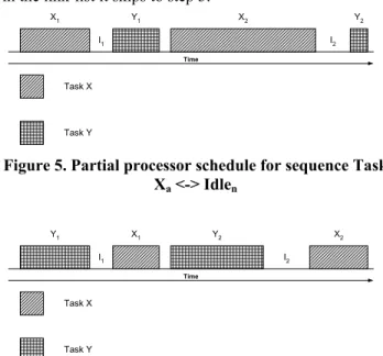
Figures 5 and 6 depict portions of the Processor schedule with the desired sequence of links shown in figures 3 and 4 respectively. If the required sequence cannot be found in the link-list it skips to step 3.
Task X Task Y X1 Y1 X2 I1 I2 Time Y2
Figure 5. Partial processor schedule for sequence Task Xa <-> Idlen Task X Task Y Y1 X1 Y2 I1 I2 Time X2
Figure 6. Partial processor schedule for sequence Idlen
<-> Task Xa
If the scheduler is unable to find a single instance of the required sequence it skips to step 3.
Once the scheduler finds a valid sequence which contains at least one Idle time link for which,
Duration(Idle Im)>= Duration (Task X)
it counts the total number of links in the sequence and the number of Idle time links. This ensures that this sequence does contain enough Idle time to accommodate at least one more channel running task X.
Let us assume that we end up with two sequences,
Task X1 <-> Idle1
Task X2 <-> Idle2
It then chooses the one with the longer duration. In this case, if,
Duration (Task X2) > Duration (Task X1)
it chooses sequence,
Task X2 <-> Idle2
and schedules the new task z as close to the right of Task X2 possible.
3. If the scheduler is still unable to schedule the channel, the scheduler abandons this Processor and checks the next best Processor the Processor Selection Algorithm returned. The scheduler repeats steps 1 and 2 for that processor. This way the scheduler loops through all the processors returned by the Processor Selection Algorithm until it finds a suitable time-slot for task z. If at the end of this search the scheduler still is not able to find a suitable time slot for the task it skips to step 4.
4. The scheduler returns to the best processor returned by the Processor Selection Algorithm and searches it for its biggest available time slot and schedules the channel in its center.
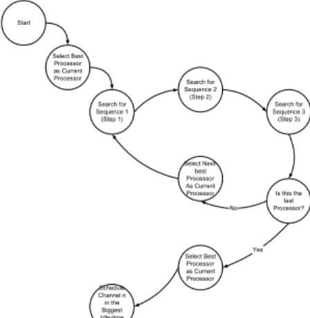
The state diagram in Figure 7 shows the sequence in which the scheduler searches for an appropriate time slot using steps 1-5 described above.
Start Search for Sequence 1 (Step 1) Select Best Processor as Current
Processor Search for Sequence 2 (Step 2) Search for Sequence 3 (Step 3) Is this the last Processor? Select Next-best Processor As Current Processor Select Best Processor as Current Processor Schedule Channel n in the Biggest Idle-time Slot No Yes
Figure 7. Sequencing of steps 1-4.
3.2.2. Task X Not Already In Use On Selected Processor(s)
If the processors returned by the Processor Selection Algorithm are of a kind which do not contain any previous channels of task type X, it follows the method outlined in this section to schedule a new task z.
It finds the Processor with the biggest Idle time slot from among the processors returned by the Processor Selection Algorithm and schedules task z in the center of the biggest available Idle time slot.
4. System Utilization Controller
It is usually desirable that processor utilization of a system be kept as high as possible. However, when the code fetch to data fetch ratio exceeds a certain limit it becomes necessary to limit the System Utilization (SU).
4.1. System Utilization
The System Utilization (SU) is calculated by,
0
Σ
N-1 (Busy time in P)SU = __________________ N x P
The value of SU is updated every time a new task is scheduled or removed.
4.2. System Utilization Limit
The System Utilization Limit (SUL) is the maximum allowable upper limit of the SU. The SUL is changed adaptively by the System Utilization Controller.
In order to keep the System Entropy (SE) within limits it is necessary to adaptively control the allowable upper limit on the SU, referred to as System Utilization Limit (SUL). The SUL is controlled by the System Utilization Controller (SUC).
4.3. System Entropy
The scheduler uses a metric called System Entropy (SE) which is an estimated measure of the system’s entropy. The higher the SE, the greater the extent to which different tasks share the same processor and the higher the number of code fetch requests. SE is a function of the average number of non-resident tasks per processor.
SE = f (Avg. num. of different task types per processor) 4.4. Lower System Utilization Threshold
The Lower System Utilization Threshold (LSUT) is the SU value at which the SUC holds down the SUL for a certain period of time until it drops below the SE limit.
4.5. System Utilization Controller State Machine
The SUC is a state machine which varies the SUL according to the SE. It updates its current state on every interrupt the scheduler is invoked. The steps followed by the SUC state machine are described below.
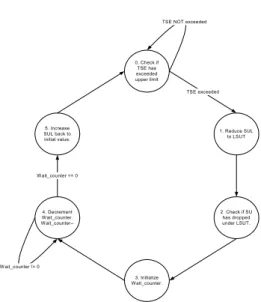
0. Check if SE has exceeded upper limit. a. SE > SUL: Jump to state 1. b. SE <= SUL: Wait in state 0. 1. Reduce SUL: Jump to state 2. 2. Check if SU has crossed LSUT.
a. SU > LSUT: Wait in state 2. b. SU <= LSUT: Jump to state 3. 3. Initialize Wait_counter: Jump to state 4. 4. Decrement Wait_counter, i.e. Wait_counter--.
a. Wait_counter ==0: Jump to state 5. b. Wait_counter!= 0: Wait in state 4. 5. Increase SUL (e.g. from 60% to 80%) back to
previous value. Jump to state 0.
0. Check if TSE has exceeded upper limit 4. Decrement W ait_counter. W ait_counter--5. Increase SUL back to initial value. 3. Initialize W ait_counter. 2. Check if SU has dropped under LSUT. 1. Reduce SUL to LSUT TSE NOT exceeded
TSE exceeded
W ait_counter != 0 W ait_counter == 0
Figure 8. SUC state machine
The graphical representation of the state machine is given figure 8.
5. Implementation Results
The CSHA was implemented in C and profiled on an intel Pentium-III 733MHz processor. The implementation supported 2048 tasks on P = 12 processors in a time period of T = 10 msec divided into S = 40 time-slots of 0.25 msec each. New task scheduling requests were being generated at the rate of calls were established at the rate of 1 every 10mSec or 100 new tasks per second.
Simulation time: 25,040 * 10 = 250,400 mSec Real time: 13,774.457 mSec
%-age time spent in functions that will not be used in the real scheduler ,i.e. file accesses, call duration counter updates related functions = 94.1%
%-age time spent in functions that will be part of the final implementation of the scheduler
= 100 - 94.1 = 5.9%
Real time spent in functions that will be part of the final implementation of the scheduler
= 5.9% of 13,774.457 = 812.69 ~= 813 mSec Processor utilization
= 100 * (Real time spent in final implementation functions/ Simulation time)
= 100 * (813mSec/ 250,400mSec) ~= 33%
6. Conclusions
From the CSHA code’s profiling results it can be seen that this algorithm can be implemented for use in real-time systems. Potential applications include multiprocessor DSP systems, i.e. radars, voice and video encoders/ decoders, in which samples of data of multiple channels are processed periodically.
7. References
[1] Albert Y. H. Zomaya, Parallel & Distributed Computing Handbook, McGraw-Hill, 1995.
[2] Charles F. Bowman, Algorithms and Data Structures – An Approach in C, Saunders College Publishing, 1993. [3] Bernard Sklar, Digital Communications -Fundamentals and Applications, PTR Prentice-Hall, 1988.
[4] J. Goossens, C. Macq, Performance Analysis of various Scheduling Algorithms for Real-ime Systems Composed of Aperiodic and Periodic Tasks, Proceedings of SCI/ISAS'99 (Orlando, FL), August, 1999.