Surface Reconstruction from Multi-View Stereo
∗ Nader Salman1 and Mariette Yvinec1INRIA Sophia Antipolis, France
Abstract. We describe an original method to reconstruct a 3D scene from a sequence of images. Our approach uses both the dense 3D point cloud extracted by multi-view stereovision and the calibrated images. It combines depth-maps construction in the image planes with surface reconstruction through restricted Delaunay triangulation. The method may handle very large scale outdoor scenes. Its accuracy has been tested on numerous scenes including the dense multi-view benchmark proposed by Strecha et al. Our results compare favorably with the current state of the art.
1
Introduction
Motivations. Various applications in Computer Vision, Computer Graphics and Computational Geometry require a surface reconstruction from a 3D point cloud extracted by stereovision from a sequence of overlapping images. These ap-plications range from preservation of historical heritage to e-commerce through computer animation, movie production and virtual reality walkthroughs.
Early work on reconstruction has been focused on data acquired through laser devices, with characteristics that the obtained 3D point cloud is dense and well distributed [1–3]. Although these reconstruction methods have been reported as succesful, the nature of the laser scanners greatly limit their usefulness for large-scale outdoor reconstructions.
The recent advances in multi-view stereovision provide an exciting alterna-tive for outdoor scenes reconstruction. However, the extracted 3D point clouds are entangled with redundancies, a large number of outliers and noise. Fortu-nately, on top of these point clouds, the additional information provided by the calibrated images can be exploited to help surface reconstruction.
In this work, our goal is to recover a meshed model from a multi-view im-age sequence. We assume that the imim-ages have been processed by a multi-view stereovision algorithm and start from the calibrated images and a set of tracks. Each track is a 3D point associated to a list of images where the point is visible. The model sought after is either a simplicial surface mesh or a 3D mesh of the objects in the scene.
∗
Work partially supported by the ANR(Agence Nationale de la Recherche)under the “Gyroviz” project (No ANR-07-AM-013)http://www.gyroviz.org
Related Work.Over the past three decades there have been significant efforts in surface reconstruction from images, typically targeting urban environments or archaeological sites. The requirements for the ability to handle large-scale scenes discards most of the multi-view stereo reconstruction algorithms including the al-gorithms listed in the Middlebury challenge [4]. The methods which have proved to be more adapted to large-scale outdoor scenes are the ones that compute and merge depth-maps [5–9]. However, in multiple situations, the reconstructed 3D models lack of accuracy or completeness due to the difficulty to take visi-bility into account consistently. Recently, two different accurate reconstruction algorithms have been proposed in [10, 11]. We demonstrate the efficiency of our reconstruction results relying on the publicly available quantitative challenge from the review of Strecha et al. [12] currently led by [10, 11].
Contributions. Our reconstruction method is close to [13] and to the image-consistent triangulation concept proposed by Morris and Kanade [14]. It consists in a pipeline that handles large-scale scenes while providing control over the density of the output mesh. A triangular depth-map is built in each image plane, respecting the main contours of the image. The triangles of all the depth-maps are then lifted in 3D, forming a 3D triangle soup. The similarity of the triangle soup with the surface of the scene is further enforced by combining both visibility and photo-consistency constraints. Lastly, a surface mesh is generated from the triangle soup using Delaunay refinement methods and the concept of restricted Delaunay triangulation. The output mesh can be refined until it meets some user-given size and quality criteria for the mesh facets. A preliminary version of this work appeared as a video in the ACM Symposium on Computational Geometry 2009 [15].
2
Basic Notions
In this section we define the concepts borrowed from computational geometry that are required for our method.
LetP ={p0, . . . , pn} be a set of points inRd that we call sites. TheVoronoi cell V(pi), associated to a site pi, is the region of points that are closer topi than to all other sites inP:
V(pi) ={p∈Rd:∀j=6 i,kp−pik ≤ kp−pjk}
The Voronoi diagram V(P) of P is a cell decomposition of Rd induced by the Voronoi cellsV(pi).
TheDelaunay complex D(P) ofPis the dual of the Voronoi diagram meaning the following. For each subsetI ⊂ P, the convex hullconv(I) is a cell ofD(P) iff the Voronoi cells of points in I have a non empty intersection. When the set P is in general position, i.e. includes no subset of d+ 2 cospherical points, any cell in the Delaunay complex is a simplex. This Delaunay complex is then a triangulation, called theDelaunay triangulation. It decomposes the convex hull ofP intod-dimensional simplices.
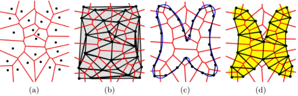
(a) (b) (c) (d)
Fig. 1: (a) the Voronoi diagram of a set of 2D points; (b) its dual Delaunay triangulation. (c) The Delaunay triangulation restricted to the blue planar closed curve is plotted in black. (d) The Delaunay triangulation restricted to the yellow region is composed of triangles whose circumcenters are inside the region.
LetΩ be a subset of Rd, we call Delaunay triangulation of P restricted to Ω and we note DΩ(P), the sub-complex of D(P), that consists of the faces of
D(P) whose dual Voronoi faces intersectΩ. This concept has been particularly fruitful in the field of surface reconstruction, whered= 3 andP is a sampling of a surface S. Indeed, it has been proven that under some assumptions, and specially ifP is a “sufficiently dense” sample ofS,DS(P) is homeomorph to the surface S and is a good approximation ofS in the Hausdorff sense [16]. Fig. 1 illustrates the notion of restricted Delaunay triangulation.
TheDelaunay refinement surface meshing algorithm builds incrementally a sampling P on the surface S whose restricted triangulation DS(P) is a good
approximation of the surfaceS. At each iteration, the algorithm inserts a new point of S into P and maintains the 3D Delaunay triangulation D(P) and its restriction DS(P). Insertion of new vertices is guided by criteria on facets of DS(P): minimum angleα; maximum edge lengthl; maximum distancedbetween
a facet an the surface. The algorithm [16] has the notable feature that the surface has to be known only through an oracle that, given a line segment, detects whether the segment intersects the surface and, if so, returns the intersection points.
At last, we also use the notion of 2D constrained Delaunay triangulation based on a notion of visibility [17]. Let G be the set of constraints forming a straight-line planar graph. Two points p and q are said to be visible from each other if the interior of segment pq does not meet any segment of G. The triangulationT inR2is a constrained Delaunay triangulation ofG, if each edge of
T is either an edge ofGor aconstrained Delaunay edge. A constrained Delaunay edge is an edgee such that there exist a circle through the endpoints ofethat encloses no vertices of T visible from an interior point ofe.
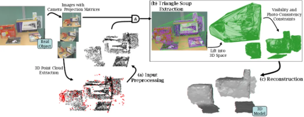
Fig. 2: Reconstruction pipeline overview. Both images and camera projection matri-ces are used by the stereo vision algorithm to extract a 3D point cloud. (a) We will first preprocess the 3D point cloud. (b) Using the preprocessed 3D points and the camera projection matrices we extract a triangle soup that minimize visibility and photo-consistency violations. (c) Finally, we use the triangle soup as a surface approxi-mation and build the output 3D model. Note that the triangles lying on the table were voluntary removed for readability.
3
The Reconstruction Algorithm
The algorithm takes as input a sequence of calibrated images and a set of tracks provided by multi-view stereo. The algorithm consists of three steps: 1) merging, filtering and smoothing the tracks, 2) building a triangle soup, and 3) computing from the triangle soup a mesh modeling the scene. The different steps of our algorithm are illustrated in Figure 2.
The following sections describe the three steps of the algorithm in more detail.
3.1 Merging, Filtering and Smoothing
Each input track stores its 3D point location as well as the list of camera locations from which it was observed during acquisition. In the following, we call line-of-sight the segment from a camera location to the 3D position of a track seen by this camera. Despite the robust matching process used by the multi-view stereo algorithm, the extracted tracks require some preprocessing including merging, filtering and smoothing.
Merging.The first preprocessing step in our method consists in merging tracks whose positions are too close with respect to some thresholdξ1. When two tracks are merged in a single one their list of cameras is updated to include the union of the cameras of the two merged tracks.
Filtering.As tracks are coming from characteristic points detected in the im-ages, their 3D locations should be densely spread over the surface of the scene objects. Thus, tracks which are rather isolated are likely to be outliers. Another criterion used to further filter out outliers, is based upon the angle between lines-of-sight. When a 3D point location is computed from lines-of-sight forming small angles, the intersection computation is imprecise and the 3D point is likely to be noisy. For these reasons we use two criteria to detect outliers in the set of tracks: Thedistance to neighbors and thecone angle.
- Distance to neighbors. We compute for each track with 3D position pi the average Euclidean distance dk1(pi) from pi to its k1-nearest neighbors and we remove a small percentage ξ2 of tracks with largest value.
- Cone angle filtering.We compute for each track with 3D positionpi the aper-ture angle of the smallest cone with apex at pi containing all cameras Ci that observe pointpi. Tracks with small cone anglesξ3are discarded.
Smoothing. The final preprocessing step smooths the remaining tracks using a smoothing algorithm based upon jet-fitting and re-projection [18]. For each track, we compute a low degree polynomial surface (typically a quadric) that approximates itsk2-nearest neighbors. We then project the track onto the com-puted surface.
In all our experiments we usedξ1= 0.001β, whereβ is the half diagonal of the bounding box of the point cloud, ξ2 is 0.06%, ξ3 = 0.08 radian, k1 = 150 andk2= 85. .
3.2 Triangle Soup Extraction
The next step in our method combines the preprocessed tracks and the input images to build in each image plane a triangular depth-map that comply with the image discontinuities. The triangles of each depth-map are then lifted into 3D space forming a triangle soup which will require further filtering to minimize violations of visibility and photo-consistency constraints.
Depth-Maps Construction Since contours in the images are natural indica-tors of surface discontinuities, it is expedient to include contour information in the depth-maps construction process. A simple yet powerful method for contour detection is to perform a contrast analysis into the input images using gradient-based techniques.
In each image, we then compute an approximation of the detected contours as a set of non-intersecting polygonal lines with vertices on the projection of the tracks. For this we consider in each image the projection of the tracks located in this image. We call contour track, orctrack, a track whose projection on the image is close to some detected contour. We call a non-contour track, ornctrack, any other track. We consider the complete graph over all ctracks of an image and select out of this graph, the edges which lay over detected contours. The selection
is performed by a simple weighting scheme using [19]. Inherently, whenever there isnctracks aligned on an image contour, we select then(n2−1)edges joining these tracks. Albeit, we wish to keep only the (n−1) edges between consecutive ctracks on the contours. For these reasons we use a length criteria to further select a subset of non-overlapping edges fashioning the polygonal approximation of the contour.
Edges in the polygonal contour approximation are used as input segments to a 2D constrained Delaunay triangulation with all projected tracks, ctracks and nctracks, as vertices. The output is a triangular depth-map per image. The triangles of this depth-map are then lifted in 3D space using the 3D coordinates computed by the multi-view stereo algorithm. However, lifted depth-maps from consecutive images partially overlap one another and the triangle soup includes redundancies. When two triangles share the same vertices, only one is kept.
Triangle Soup Filtering The vast majority – but not all – triangles of the soup lie on the actual surface of the scene. In the sequel, we note ∆ ={T0, . . . , Tn} the 3D triangle soup. We wish to filter ∆to remove erroneous triangles. (1) Thevisibility constraint states that the line-of-sight from a camera position to the 3D position of a track seen by this camera belongs to the empty space, i.e., it does not intersect any object in the scene. Therefore a triangle intersected by some line-of-sight should be removed from ∆. However, this rule has to be slightly softened to take into account the smoothing step (Section 3.1) where the tracks 3D positions have been slightly changed. More specifically, each triangle Ti in ∆ gets a weightwi equal to the number of lines-of-sight intersecting Ti. We then discard from∆ any triangle with a weightwigreater than a threshold ξ4.
(2) We also filter out any triangle whose vertices, at least one of them, are only seen by grazing lines-of-sight. In practice, an angle greater than 80 degrees between the line-of-sight and the triangles normal is used in all our experiments to characterise a grazing line-of-sight.
(3) Depending on the density of the preprocessed tracks, the triangle soup can contain “big” triangles, i.e. triangles whose circumradii are big compared to the scale of the scene. We use shape andphoto-consistency constraints to filter big triangles.
A triangle is said to beanamorphicif it has a too big radius-edge ratio,where the radius-edge ratio of a triangle is the ratio between the radius of its circum-circle and the length of its shortest edge. Anamorphic big triangles are likely to lie in free space and should be discarded.Big triangles with regular shapes are filtered using photo-consistency criteria: A 3D triangle Ti in ∆ is photo-consistent, if its projections into all images where Ti vertices are visible, corre-spond to image regions with the same “texture”. To decide on photo-consistency, two common criteria are Sum of the Squared Difference (SSD) and Normalsed Cross-Correlation (NCC) between pixels inside the projected triangle in each image. In our experiments we use NCC because it is less sensitive to illumina-tion change between the views. We only use images where the angle between the
normal of the 3D triangle and the line-of-sight through the center of the image is small. This scheme gives head-on view more importance than oblique views.
3.3 Reconstruction
For the final step, we use the Delaunay refinement surface mesh generation algo-rithm [16] described in Section 2. Recall that this algoalgo-rithm needs to know the surface to be meshed only through an oracle that, given a line segment, detects whether the segment intersects the surface and, if so, returns the intersection points. We implemented the oracle required by the meshing algorithm using the triangles of∆as an approximation of the surfaces. Thus, the oracle will test and compute the intersections with∆to answer to the algorithm queries.
4
Implementation and Results
The presented algorithm was implemented in C++, using bothCImgandCgal libraries.
TheCgal library [20] defines all the needed geometric primitives and pro-vides performant algorithms to compute Delaunay triangulations in both 2D and 3D [21]. It provides all the elementary operations needed in the different steps of our algorithm: vertex insertion, vertex move, nearest neighbour query, vari-ous traversal queries and point set processing [22]. Moreover, theCgallibrary provides access to the AABB tree and the general triangulation data structures (C2T3) used respectively to store the triangle soup and the surface mesh. More importantly it provides us the Delaunay refinement surface meshing algorithm that we use in the last step of our algorithm.
TheCImg library (http://cimg.sourceforge.net) is a toolkit for image processing that defines simpleclassesandmethodsto manipulate generic images. In our code we use it for the contour detection, the constraint retrieval and the photoconsistency filtering step.
In our experiments, we used for the point cloud preprocessing step the param-eters (ξ1, ξ2, ξ3, k1, k2) values as listed at the end of Section 3.1. Moreover, the visibility constraint thresholdξ4, defined in Section 3.2, is set at 5 rays. Leaving aside the time required by the multi-view stereo processing (image calibration and track extraction), in our experiments the runtime of our reconstruction al-gorithm ranges from 9 minutes for 200 000 tracks on 8 images to 35 minutes for 700 000 tracks on 25 images on an IntelRQuad Xeon 3.0GHz PC.
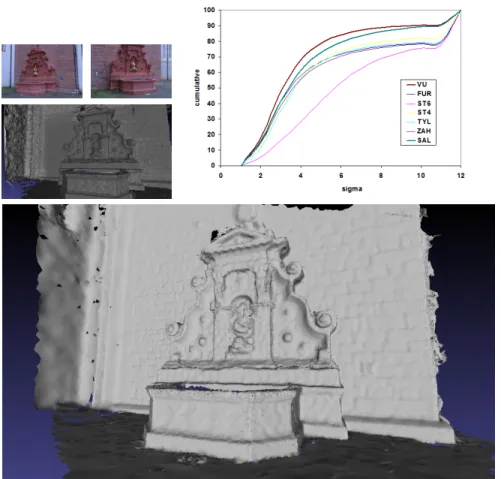
Strecha et al. [12] provide quantitative evaluations for six outdoor scene datasets. The evaluation of the reconstructed models is quantified through the cumulative error distribution, showing, for each deviation σ, the percentage of the scene recovered within an error less thanσ. The deviation is estimated with respect to the ground truth model acquired with a LIDAR system. We have tested our approach on thefountain-p11,entry-p10, castle-p19 and Herz-Jesu-p25 particularly challenging datasets. Focusing on the fountain-p11 dataset, Fig. 3 shows, two of the images, the extracted triangle soup, our reconstruction
Fig. 3: Top-left: 2 images of fountain-p11 and the extracted triangle soup. Bottom: our reconstruction (500 000 triangles). Top-right: the cumulative error distribution (SAL for our work) compared with VU [11], FUR [10], ST4 [5], ST6 [6], ZAH [23] and TYL [9].
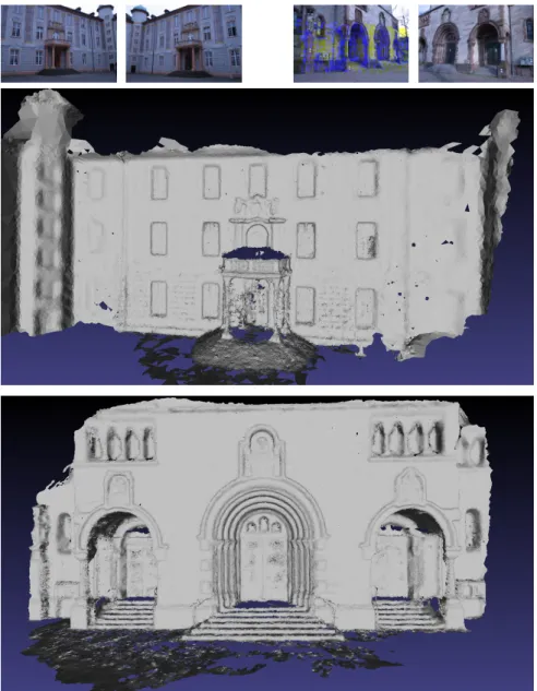
and the cumulative error distribution compared with the distributions for other reconstructed methods. The stereovision cloud has 392 000 tracks from which 35 percent were eliminated at the preprocessing step. Our algorithm has succesfully reconstructed various surface features such as regions of high curvature and shal-low details while maintaining a small number of triangles. The comparison with other methods [5, 6, 9–11, 23] shows the versatility of our method as it generates small meshes that are more accurate and complete than most of the state-of-art while being visually acceptable. Fig. 5 shows our reconstruction results for the entry-p10 and the Herz-Jesu-p25 datasets. For extended results we refer the reader to the challenge website [12].
To show the ability of our algorithm to cope with much bigger outdoor scenes and its ability to produce meshes that take into account the user budget for the
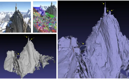
Fig. 4: On the left: two images of theAiguille du midi dataset ( cB.Vallet/IMAGINE); below: our low resolution reconstruction (270 000 triangles). On the right: our high resolution reconstruction (1 000 000 triangles). Note how most details pointed by yellow arrows are recovered in both resolutions.
size of the output mesh, we have chosen to test our method on the Aiguille du Midi dataset ( cB.Valet/IMAGINE). It includes 51 images, the extracted cloud has 6 700 000 points with lots of outliers. At the preprocessing step, 80 percent of the points were eliminated. The Delaunay refinement surface meshing is tuned through three parameters: the angular boundα controls the shape of the mesh facets, the distance d and the size parameter l govern respectively the approximation accuracy and the size of mesh elements. The reconstructions shown in Fig. 4 are obtained with αequals 20 degrees and d, l respectively set as (0.01, 0.035) and (0.002, 0.01) in unit of the bounding box half diagonal. We have tuned parametersdandlto adapt the mesh to a targeted size budget. This enabled us to reconstruct from a single extracted triangle soup output meshes of various resolutions (270 000 triangles and 1 000 000 triangles respectively in Fig. 4). Note that details such as antenas and bridges are recovered even in the coarsest model.
5
Conclusion
In this paper, we have proposed a novel 3D mesh reconstruction algorithm com-bining the advantages of stereovision with the power of Delaunay refinement surface meshing. Visual and quantitative assessments applied on various large-scale datasets indicate the good performance of our algorithm. As for ongoing
work, we want to explore the possibility to automatically pre-compute the thresh-olds such as (ξ1, ξ2, ξ3, ξ4) from the images and incorporate in the reconstruction process a scale dependent sharp edges detection and recovery procedure to build geometrically simplified models.
Acknowledgments
We wish to thank Renaud Keriven and Jean-Philippe Pons for their point cloud extraction software and the Aiguille du Midi dataset, Laurent Saboret for his precious collaboration and Christoph Strecha for his challenge and his kind help.
References
1. Ohtake, Y., Belyaev, A., Alexa, M., Turk, G., Seidel, H.P.: Multi-level partition of unity implicits. In: Proc. of ACM SIGGRAPH. (2003)
2. Kazhdan, M., Bolitho, M., Hoppe, H.: Poisson Surface Reconstruction. In: Proc. of SGP ’06. (2006)
3. Hornung, A., Kobbelt, L.: Robust reconstruction of watertight 3D models from non-uniformly sampled point clouds without normal information. In: Proc. of SGP ’06. (2006)
4. Seitz, S.M., Curless, B., Diebel, J., Scharstein, D., Szeliski, R.: A comparison and evaluation of multi-view stereo reconstruction algorithms. In: Proc. of CVPR ’06 5. Strecha, C., Fransens, R., Van Gool, L.: Wide-baseline stereo from multiple views:
a probabilistic account. In: Proc. of CVPR ’04. (2004)
6. Strecha, C., Fransens, R., Van Gool, L.: Combined depth and outlier estimation in multi-view stereo. In: Proc. of CVPR ’06. (2006)
7. Goesele, M., Snavely, N., Curless, B., Hoppe, H., Seitz, S.: Multi-view stereo for community photo collections. In: Proc. of ICCV ’07. (2007)
8. Pollefeys, M., Nister, D., Frahm, J., Akbarzadeh, A., Mordohai, P., Clipp, B., Engels, C., Gallup, D., Kim, S., Merrell, P., et al.: Detailed real-time urban 3d reconstruction from video. International Journal of Computer Vision (2008) 9. Tylecek, R., Sara, R.: Depth map fusion with camera position refinement. In:
Computer Vision Winter Workshop. (2009)
10. Furukawa, Y., Ponce, J.: Accurate, dense, and robust multiview stereopsis. In: Proc. of CVPR ’07. (2007)
11. Vu, H., Keriven, R., Labatut, P., Pons, J.P.: Towards high-resolution large-scale multi-view stereo. In: Proc. of CVPR ’09. (2009)
12. Strecha, C., von Hansen, W., Van Gool, L., Fua, P., Thoennessen, U.: On bench-marking camera calibration and multi-view stereo for high resolution imagery. Proc. of CVPR ’08 http://cvlab.epfl.ch/ strecha/multiview/denseMVS.html. 13. Hilton, A.: Scene modelling from sparse 3d data. Image and Vision Computing
23(10) (2005) 900 – 920
14. Morris, D., Kanade, T.: Image-consistent surface triangulation. In: Proc. of CVPR ’00. (2000)
15. Salman, N., Yvinec, M.: High resolution surface reconstruction from overlapping multiple-views. In: SCG ’09: Proceedings of the 25th annual symposium on Com-putational geometry, New York, NY, USA, ACM (2009) 104–105
16. Boissonnat, J.D., Oudot, S.: Provably good sampling and meshing of surfaces. Graphical Models (2005)
17. de Berg, M., Cheong, O., Overmars, M., Van Kreveld, M.: Computational Geom-etry – Algorithms and Aplications (3rd). Springer-Verlag Berlin (2008)
18. Cazals, F., Pouget, M.: Estimating differential quantities using polynomial fitting of osculating jets. In: Proc. of SGP ’03. (2003)
19. Needleman, S.B., Wunsch, C.D.: A general method applicable to the search for similarities in the amino acid sequence of two proteins. J Mol Biol48(1970) 20. Cgal, Computational Geometry Algorithms Library http://www.cgal.org. 21. Boissonnat, J.D., Devillers, O., Teillaud, M., Yvinec, M.: Triangulations in cgal
(extended abstract). In: Proc. of SCG ’00. (2000)
22. Alliez, P., Saboret, L., Salman, N.: Point set processing. In Board, C.E., ed.: CGAL User and Reference Manual. 3.5 edn. (2009)
23. Zaharescu, A., Boyer, E., Horaud, R.: Transformesh: a topology-adaptive mesh-based approach to surface evolution. In: Proc. of ACCV ’07. (2007)
Fig. 5: Top to bottom: 2 images of entry-p10 and 2 images of Herz-Jesu-p25; our reconstruction of entry-p10 (500 000 triangles); our reconstruction of Herz-Jesu-p25 (1 200 000 triangles).