News-Related Social Media Use,
Political Knowledge, and Participation in the 2016 Election
By John Roberson
Senior Honors Thesis Department of Public Policy University of North Carolina at Chapel Hill
April 26, 2019
Approved:
. .
Douglas Lee Lauen, Thesis Advisor
.
Abstract
Social media’s role in the 2016 election was one of many aspects of that election which make it unique. Record numbers of Americans were active social media users in 2015-2016, and many used the platforms not only for entertainment, but to learn about the news. Social media were also used by candidates in novel ways and to unprecedented extents, and the quality of
information distributed through social media came into question. Previous studies have shown that news-related social media use leads to increases in political knowledge and likelihood of voting, but the unique circumstances surrounding the 2016 election make generalization of those findings to that election perilous. Therefore, this thesis used national survey data from the 2016 Cooperative Congressional Election Survey to investigate the relationships between news-related social media use, political knowledge, and participation specifically in the 2016 election.
Acknowledgments
First, I want to thank my advisor, Dr. Doug Lauen. His patience during the conceptual phase of this thesis let me arrive at a final topic to which I could give my full effort, and his advice throughout the remainder of the process always kept me on the right path. I am especially grateful for his guidance and willingness to think through problems with me because the topic of my research falls outside of his typical domain. I would also like to thank my second reader, Dr. Rebecca Kreitzer, who not only is the person who first brought the Cooperative Congressional Election Survey to my attention as a potential data source, but who never failed to have valuable, actionable advice every time we spoke.
I also want to thank my family and friends for their support throughout this process, and for never telling me that I talked about my thesis too much, though I know I did. I am so grateful for my roommate and best friend, Bailey, who went through the thesis-writing experience
TABLE OF CONTENTS
INTRODUCTION... 1
1. Web 2.0, Social Media, and a Shift in the Flow of Information ... 2
2. Policy Relevance ... 3
3. The 2016 Election ... 6
4. Key Research Questions ... 8
5. Thesis Roadmap ... 9
BACKGROUND ... 10
1. Social Media Use ... 10
2. Political Knowledge ... 13
3. Political Participation ... 19
4. Putting It All Together ... 20
METHODS ... 27
1. Causal Diagram ... 27
2. The 2016 Cooperative Congressional Election Survey (CCES) ... 29
2 A. Vote Validation in the CCES ... 31
3. Modeling Social Media Behavior ... 37
4. Modeling Political Knowledge ... 44
5. Other Selected Variables for Analysis ... 48
6. Regression Models ... 50
RESULTS ... 53
1. Descriptive Analysis ... 53
2. Regression of Voting on Social Media News Use ... 59
3. Regressions of Political Knowledge on Social Media News Use ... 69
CONCLUSIONS ... 72
1. Evaluation of Hypotheses ... 72
2. Limitations of Methods ... 74
3. Implications of Findings ... 75
4. Suggestions for Future Research ... 77
REFERENCES ... 80
APPENDIX A: FACTOR ANALYSIS OUTPUT ... 92
TABLE OF TABLES
Table 1: Determinants of Political Knowledge ... 16
Table 2: Summary of Potential Confounding Variables ... 26
Table 3: Defining Three Validated Voter-Turnout Measures ... 34
Table 4: Selecting a Validated Voter-Turnout Measure ... 36
Table 5: Social Media Behavior EFA Results ... 42
Table 6: Political Knowledge EFA Results ... 47
Table 7: Descriptions of Voting Regression Models ... 51
Table 8: Weighted Descriptive Statistics of Key Variables ... 53
Table 9: Exponentiated Coefficients on Treatment and Mediating Variables, Logit Regressions of Voting on Social Media Use ... 60
Table 10: Frequency Distribution of Social Media Use Response Patterns ... 92
Table 11: Social Media Behavior Preliminary EFA Results A ... 93
Table 12: Social Media Behavior Preliminary EFA Results B ... 93
Table 13: Social Media Behavior EFA Results - No Omitted Loadings ... 93
Table 14: Frequency Distribution of Political Knowledge Response Patterns ... 94
Table 15: Political Knowledge Preliminary EFA Results A ... 95
Table 16: Political Knowledge Preliminary EFA Results B ... 95
Table 17: Political Knowledge EFA Results – No Omitted Loadings ... 95
Table 18: Full Logit Regressions of Voting on Social Media, Mediated and Unmediated, with and without State Fixed Effects ... 96
TABLE OF FIGURES
Figure 1: The Mediated Relationship Between Social Media News Consumption and Voting .. 28
Figure 2: Social Media EFA Loadings, Before and After Rotation ... 41
Figure 3: Kernel Densities of SM Factor Scores ... 43
Figure 4: Age Distributions by Model Sample ... 55
Figure 5: Distribution of Social Media Consumption by Model Sample ... 56
Figure 6: Distribution of Social Media Engagement by Model Sample ... 56
Figure 7: Distribution of Personal Knowledge Scores by Model Sample ... 56
Figure 8: Distribution of General Knowledge Scores by Model Sample ... 56
Figure 9: Distribution of Educational Attainment by Model Sample ... 57
Figure 10: Income Distribution in Analytical Sample ... 57
Figure 11: Ideological Distribution by Model Sample ... 58
Figure 12: Distribution of Party Identifications by Model Sample ... 58
Figure 13: Party IDs of Self-Reported Ideological Moderates ... 59
Figure 14: Odds Ratios Across Mediated Models of Voting (Comparing Methods for Calculating Political Knowledge) ... 61
Figure 15: Predictive Margins of Consumption on Voting, by Level of Active Engagement .... 62
Figure 16: Contrasts of Predictive Margins of PersonalKnowledge on Voting ... 64
Figure 17: Heatmaps of Statewide Turnout and State-Level Contrasts in Predicted Turnout by Level of Social Media News Consumption ... 65
Figure 18: Scatterplot of Statewide Turnout against State-Level Contrasts in Predicted Turnout by Level of Social Media News Consumption ... 66
Figure 19: Odds Ratios Across Split Models of Voting by Party ID (Comparing Models Limited to only Democrats and only Republicans) ... 67
Figure 20: Predictive Margins of Social Media News Consumption on Voting by Level of Active Engagement, across Separate Models for Democrats and Republicans ... 68
Figure 21: Predictive Margins of Social Media News Consumption on Personal Political Knowledge, by Level of Active Engagement ... 69
Figure 22: Predictive Margins of Age on PersonalKnowledge Score ... 70
Introduction
Social media is pervasive in many Americans’ daily lives in 2019. To some, it is a way to connect with old friends; to others, a way to catalog their daily experiences; and to many others, something different. One marked change in social media over the last decade is the development of social networking sites as platforms for the dissemination of news. Traditional news outlets have inserted themselves into the social media sphere and are one source of the news information that is spread across social networking sites, but such sites are also part of Web 2.0 at their core – and as such, any site member is empowered to be a source of information as well, with varying degrees of influence based on the size of their networks. People and media companies share all kinds of news over social media, but whenever “news” is referred to in the rest of this thesis, it should be assumed that the term refers to political news specifically.
1. Web 2.0, Social Media, and a Shift in the Flow of Information
Until the 1980s, information mainly was spread one of a few ways: through mass media, through education, or by word of mouth. In that traditional media context, word-of-mouth
information spread was limited, and information flowed in society unidirectionally, flowing from a few mass media producers to mass consumers (Mandiberg 2012, 1). Starting in the 1980s, technologies like photocopiers, home video cameras, and home computing began allowing one person’s information to reach more people without going through mass media (1). Soon after that came a boom in home computing, which brought mass access to the internet and dramatically increased people’s connectivity with the outside world. Still, that connectivity was limited.
It can be said that the internet so far has developed through two eras (and is arguably about to enter a third). A 2012 blog post from a web design studio provides an oversimplified, but useful way to distinguish the eras: in computer science language, Web 1.0 was the “readable” era of the internet, Web 2.0 is the “writable” phase, and, while not really realized yet, Web 3.0 will be the “executable” phase of the internet (WittyCookie 2012). In more detail, “Web 1.0,” was mostly a one-way street. Sites made information available to users, but users had little to no opportunity to return the favor. In Web 2.0, the internet is a two-way street: sites provide users with information, users make use of it and provide information back to the sites, sites update their services based on the received data, and the cycle continues (O’Reilly 2007). Importantly, this process introduced the possibility of not only making one user’s data available to the website, but to other users of the site as well – the birth of social media (Mandiberg 2012, 2).
Buckingham, a giant of turn-of-the-century media literacy scholarship, describes this very clearly, writing about the general consensus that
the interactive, participatory possibilities of digital media are believed to transcend the limitations of hierarchical, top-down ‘mass’ media and hence to undermine what are seen as the authoritarian ‘knowledge politics’ of traditional pedagogy. The potential they offer for learners to become creators of knowledge – rather than merely ‘consumers’ has been seen by some as little short of revolutionary. (Buckingham 2015, 9)
Jay Rosen (2007) describes a similar phenomenon, writing a fictional open letter to media producers in the voice of “the people formerly known as the audience.” In that letter, he tells mass media “You don’t own the eyeballs. You don’t own the press, which is now divided into pro and amateur zones. You don’t control production on the new platform, which isn’t one-way. There’s a new balance of power between you and us” (15).
2. Policy Relevance
“Welcome to the second decade of the 21st century,” Ernest Morrell writes in 2012, “where information has been globalized, digitized, and sped up to move at the speed of thought” (300). The Pew Research Center estimates that nine in ten Americans use the internet in 2018, up from only half of the population in 2000 (Pew 2018a). There are certainly exceptions, groups that are less connected than the average (primarily older, rural Americans), but even those disparities are rapidly disappearing (Pew 2018a).
Certain social media platforms are more popular than others. By far the most popular is Facebook: 68% of Americans report using that platform, compared to 35% using Instagram, 29% using Pinterest, 27% using Snapchat, 25% using LinkedIn, and 24% using Twitter (Smith & Anderson 2018, 2). Facebook has been the most popular site in every Pew survey since the Center began asking about respondents’ use of specific social media sites in 2012, always being used by roughly three times as many people as the next-most popular site (2).
These people not only “use” the sites; most use them daily. 74% of Facebook users report using the site at least once a day, and two thirds of those report using it more than once a day. That amounts to over a third of Americans using Facebook “several times a day,” a figure that did not change significantly from 2016 to 2018 (4-5). The shares of Snapchat, Instagram, and Twitter users who use those sites daily are smaller than for Facebook, but still significant: roughly 60% for Snapchat and Instagram and 46% for Twitter (4).
Additionally, Americans do not silo themselves onto only one of these platforms. Just shy of three-quarters of Americans use more than one platform, and the median American uses three (5). Lastly, although more people would find it “not hard to give up” social media than would find it “hard” (59% versus 40%), the share of users who would find it hard has grown over recent surveys, from 28% in January 2014 (6).
All of this social media use is not purely for entertainment. Before the 2008 presidential election, political organizing and news-sharing over the most popular social media site,
the realm of politics to a budding form of political communication” (632). Contemporary traditional media outlets and scholars alike were struck by the role of social media (namely, Facebook) in the election; Woolley, Limperos, and Oliver (2010) highlight one CNN headline that questioned “Will the 2008 presidential election be won on Facebook?” (632).
Since 2008, receiving news content via social media has been on the rise. A 2017 Pew Research Center study found that two-thirds of Americans get at least some of their news on social media, with one in five Americans doing so “often” (Shearer & Gottfried 2017, 2). Much of this growth was driven by an increase in older, less-educated, and non-white Americans getting news from social media (2). For example, over half of Americans aged 50+ reported getting at least some of their news from social media sites for the first time since the question first asked in Pew surveys in 2013 (2, 14-15). For Americans under the age of 50, the share of people who got news via social media was over 75% (2).
Any government has an intrinsic interest in knowing how information spreads though its society, and that interest is even stronger when the outcome in question (civic participation) is the foundation of the system of government. With over 90% of Americans online and consuming massive amounts of information each year, it is important to understand how that information might affect their decision to vote.
into the hands of large media companies, and increased national preference for more attractive, gregarious candidates (Lang & Lang 2002, Bagdikian 1983). The introduction of internet media brought the novel concern of echo chambers; when people are given a wide set of possible news sources to choose from, scholars were concerned that people would self-select into clusters of people already more like themselves (Sunstein 2007). Now, in the social media age, a new concern has arisen, in addition to the existing ones, which deals with the extent of the average person’s influence on others: most people can make and share content in the blink of eye, some with a similar reach to many traditional media sources just half a century ago (Morrell 2012; Gil de Zúñiga et al. 2014; Allcott & Gentzkow 2017).
3. The 2016 Election
The 2016 election was exceptional in many regards, and since November 2016,
academics have worked to understand that election and the forces that shaped it. A plethora of perspectives on that election have been put forward, and the field of thought only continues to expand. Daniel Kreiss (of UNC’s Media and Journalism School) reviewed three books that lay out three of the leading perspectives on the 2016 election: that hackers (foreign and domestic) had great potential to set the national press agenda (Jamieson 2018); that changing
demographics, a fractured Republican Party, and “explicit racial appeals” made by candidate Trump combined to radicalize the election and activate key voting blocs (Sides, Tesler, & Vavreck 2018); and that “Fake news entrepreneurs, Russians, the Facebook algorithm, and online echo chambers” led to a “crisis of disinformation and misinformation” primarily in the right media ecosystem (Benkler, Faris, & Roberts 2018, 11, 15). Benkler, Faris, and Roberts (2018) provide evidence of meaningful differences between left- and right-wing media
the left includes not only left-slanted media but centric media and slanted media that nonetheless adhere to journalistic norms, while the right-slanted “ecosystem is both more isolated from the center and there are few journalistic breaks on falsity” (Kreiss 2019, 3).
One common thread through each of these perspectives is social media. Hackers, “fake news entrepreneurs,” foreign interests, and simple partisans populated echo chambers, which directly influenced social media users and also often served as source material for (mostly right-wing) which picked up the content in a “propaganda feedback loop.” Social media also did not only benefit the non-traditional, populist candidate who ultimately won the US presidency, it also played a significant role in the achievements of an unsuccessful populist candidate (Bernie Sanders) in the Democratic primary (Groshek & Koc-Michalska 2017). The full extent of social media’s impact in 2016 continues and will continue to be hashed out, but it appears that there is consensus that it did have an important effect.
methodology. As already mentioned, making the distinction between “real” and “fake” news is beyond the scope of this thesis. Nonetheless, knowing the extent to which people’s voting is affected by any news they consume over social media – valuable for policymakers and social media providers in its own right – can also give insight to the possible extent of any effect of “fake” news that might have been consumed as part of that.
4. Key Research Questions
In a media environment where Americans can get news not only from television, the newspaper, or talk radio, but also across social media, where it may be more or less filtered, personalized, biased, or detailed, what effect does that news have on Americans’ likelihood to participate in the political process? And importantly, does getting news information from social media make people more knowledgeable about politics, which one would hope that people participating in the political process would be?
Based on previous work in this field, the following hypotheses were formulated:
H1: Consuming news through social media was positively related to voting in 2016. H2: The effect of social media news use on voting in 2016 was partially mediated by an increase in political knowledge.
H3: News-related social media use will have affected Democrats and Republicans differently in 2016.
Additionally, I formulated two further hypotheses dealing with questions of measurement – the reason for this consideration is explained in Chapter Two:
H4: Measures of political knowledge which are limited only to actual attempted answers will be subject to less bias on the basis of sex.
5. Thesis Roadmap
This thesis is organized into four remaining chapters. In the next chapter, I examine past research, with a primary focus on uncovering potential confounding factors that affect two or more of: consumption of social media news content, political knowledge level, and likelihood to vote. I also review a few papers that have undertaken research questions similar to those posed by this thesis. In Chapter Three, I construct a causal diagram to explain the relationships between social media use, political knowledge, likelihood to vote, and the confounds uncovered in
Chapter Two. Then, I introduce the data used, the 2016 Cooperative Congressional Election Survey (CCES) Common Content. I review preprocessing steps taken and explain two exploratory factor analyses that were performed to obtain scores for social media use and
Background
In order to isolate the relationship between social media news use and voting, all plausible factors linking the two must be uncovered. After adding in political knowledge, all plausible factors linking it to either or both previous two must be explored as well. In this chapter, I undertake that exploration in three parts, documenting the predictors of each variable independently. At the end of the chapter, I review the literature that has previously investigated the places where those predictors overlap.
1. Social Media Use
Previous scholarly work that attempts to predict social media use falls into three main categories: psychological, network-based, and demographic. Because the CCES does not contain any psychological or social-network questions, the literature in those two categories is of limited assistance to this thesis. Nonetheless, I briefly review the highest points of the psychological papers below and extract a few useful notes. Then, I review in greater depth the papers that examine social media use from a demographic perspective.
Psychologists generally agree that personality predicts a considerable amount of social media behavior (Moore & McElroy 2011; Correa, Hinsley, & Gil de Zúñiga 2010; Ross et al. 2009). When discussing “personality,” contemporary psychologists frequently use the Five Factor Model to provide structure to their work, according to Moore and McElroy (2011, 268). The Five Factor Model delineates personality along five axes: extraversion, agreeableness, conscientiousness, emotional stability, and openness to new experiences.
employ exploratory factor analysis to create social media scales, which supports the methods of this thesis. Nonetheless, habits must be formed, and Khang, et al. (2014) offer little to explain who develops social media use habits. The Five Factor personality model might explain how people enter into social media habits, but demographic factors may explain part of it as well. Scott et al. (2017), which is explored below as part of the category of papers using demographic predictors of social media, focuses in particular on the characteristics of those social media users who “habitually engage” (312).
Moore & McElroy (2011) of the psychological category present one finding that is useful in establishing explanatory variables that will be included in this thesis: they find evidence that gender is a strong predictor of Facebook usage and content, and they suggest that it should be controlled for in future work (272). Demographically-focused papers that are cited below extend this effect from Facebook to all social media platforms.
However, as stated before, the majority of the psychological school’s findings do not factor into this thesis. This is ultimately a constraint imposed by the observational design of this thesis; the CCES simply does not ask any questions that could be used to evaluate respondents’ personalities in any robust way. It does ask personal opinion questions, e.g. what the respondent thinks government priorities should be, but none would translate cleanly into psychological models. Additionally, demographic controls will not control for personality; the most predictive personality traits, primarily extraversion, have been found to be relatively randomly distributed among demographic groups (Goldberg, et al. 1998, 399). Ultimately, differences in personality must be left in residuals in this thesis’ analysis.
al. 2017, Duggan & Brenner 2013, Lenhart, et al. 2010). This thesis relies mostly on the work of Scott et al. (2017), which attempted to create profiles of social media users among “emerging adults,” people aged 18-26. Their work contributes several explanatory variables for social media use, as well as introduces a framework for considering “active” social media use, a distinction similar to the consumption versus active engagement dynamic in question in this thesis.
In their methods, Scott et al. (2017) distinguish between two dimensions of social media use: frequency and engagement (312). “Frequency,” which according to Scott et al. (2017) is the focus of “the vast majority” of previous studies in the field, entails minutes of use, frequency counts of checking feeds, and so on. “Engagement,” on the other hand, entails responding to other users, (re)posting content, and filtering content by blocking, unfriending, or unfollowing. This “participative,” habitual engagement through social media is the active social media behavior that this thesis uses to distinguishes from basic social media news consumption.
In their results, Scott et al. (2017) find that gender, race, and education are all statistically significant predictors of social media use, though their effects are split between frequency and engagement (316, Tables 5-6). Scott et al. (2017) find that women make up a statistically-significantly greater portion of high-frequency users than low-frequency users, but find that – among people who log on at roughly equal frequencies – gender did not affect the extent to which they engaged with content by interacting with other users, posting, and so on. However, Scott et al. (2017) did find that engagement was associated with both race and education, with highly-engaged users tending to be white and more highly-educated.
age-unlimited sample than in a sample limited to people in early young adulthood. Therefore, both age and income could very possibly be significant predictors of social media use in the wider American public even though Scott et al.’s (2017) findings suggest otherwise.
Evidence to that fact is provided by multiple surveys conducted by the Pew Research Center. Smith and Anderson (2018) find “substantial differences in social media use by age” (3). Specifically, they find that social media use and age are negatively related: the older someone is, the less likely they are to use social media. 88% of those aged 18-29 use some form of social media, compared to 78% among 30 to 49 year-olds, 64% among 50 to 64 year-olds, and 37% among those aged 65 and over. Shearer and Gottfried (2018) find that 45% of American adults over the age of 50 got news from social media sites in a survey conducted in 2016, while 78% of Americans ages 18-49 got news from social media. Shearer and Gottfried’s (2018) findings also support education as a predictor of social media news use: 60% of Americans with some college experience or less education reported getting news from social media sites in that same survey, compared to 68% of college graduates and higher who reported doing so.
2. Political Knowledge
civic questions; those are explored in greater detail below. Factual questions are less common, perhaps due to their limited “staying” power. For example, the 2007 Pew survey asked
respondents to estimate the number of U.S. troops who had been killed in Iraq at the time1 and to identify the subject country of “many recent news stories about tainted food and dangerous toys2” (6-8). Such questions are useful for evaluating knowledge of “hot topics,” but because hot topics by definition come and go, using them to evaluate trends is, relatively, more difficult than identification and civic knowledge, whose questions remain essentially constant.
Civic questions ask respondents about structures, rules, and history of American
government. For example, a 2018 Pew survey categorized respondents as having either “High,” “Medium,” or “Low” civic knowledge based on their answers to four questions: who breaks tied votes in the U.S. Senate, how many votes are needed to end a filibuster in the Senate, which amendment to the Constitution sets presidential term limits, and what the Electoral College is (Pew 2018b, 117). A 2014 survey by the Annenberg Public Policy Center (APPC) asked similar questions, such as the vote threshold for presidential veto overrides, the names of the three branches of federal government, and the degree of federal and legislative oversight over the Supreme Court (APPC 2014, 1). Performance on these questions varies. Around a third of Americans could name all three branches of government in the 2014 APPC survey, but also around a third could not name even one (1). Only a quarter of Americans knew that two-thirds of both the House and Senate must vote to override a presidential veto (1). On the Pew survey, only 23% of Americans answered all four questions correctly; 44% answered two to three questions correctly, and 32% were correct on one or none (Pew 2018b, 117).
1 Around 3,500
Identification questions ask more contemporary questions about the state of politics: for example, can the respondent correctly identify which party is in control of a given legislative body? Brennan cites such a statistic in his book, claiming that “citizens generally don’t know which party controls Congress” (Chapter 2, 2). Numerous surveys put this claim to the test, and the results are mixed. The 2014 APPC survey supported Brennan’s claim, finding that 38% of Americans correctly identified the party in control of the House3 at the time; the same percent did so for the Senate4,5 (APPC 2014, 2). A 2018 Pew Research Center study contradicted Brennan’s claim, however: 82% of its survey respondents correctly identified the Republican majority in the House and 83% identified the Republican majority in the Senate. 75% correctly identified both (Pew 2018b, 108). There are many potential explanations for this difference, including difference in time frame (2014 vs. 2018) or sampling bias. It is unlikely for such a large difference to be the result of change over time, but the changed nature of politics after the 2016 election may contribute to the difference.
When asked to identify the party of their personal Representative in Congress, Americans typically answer correctly about half the time. A 2017 study found that 56% of respondents claimed to know the party of their district’s current member of Congress (Freiling 2017). It is worth noting that their claim was not validated; the 56% figure represents claims of knowledge, not verifiable knowledge. Therefore, those figures should be taken with a grain of salt.
When it comes to predictors of political knowledge, Brennan uses identification-type questions (as opposed to civic or factual questions). He identifies eight specific axes along which
3 The Republicans
4 The Democrats
such political knowledge varies, which are summarized in Table 1 below. According to his findings, political knowledge is significantly associated with many fundamental demographic factors, ranging from the relatively more-malleable, e.g. education and geographic region, to the immutable, e.g. age and race.
Table 1: Determinants of Political Knowledge
Characteristic Knowledge Positively Correlated With… Knowledge Negatively Correlated With…
Education Having a college degree Having a H.S. diploma or less
Income Earning above-average income; also being in top 25% of income earners
Earning below-average income; also being in the bottom 25% of income earners
Region of the US Living in the West Living in the South
Partisanship Being or leaning Republican Being a Democrat or leaning Independent Age Being middle-aged (35-54) Being any other age
Race - Being black
Gender - Being female
SOURCE: Brennan “Against Democracy” 2016, Chapter 2, Page 7
A 2018 Pew Research Center survey supports several of Brennan’s claims (Pew 2018b, 110). It found a positive, linear relationship between educational attainment and “civic
knowledge,” suggesting that someone with a postgraduate degree is almost four times more likely to have “high” civic knowledge than someone with a high school diploma or less. It also found that age was associated with civic knowledge, though it observed a positive, linear relationship in contrast to the parametric relationship posited by Brennan (108).
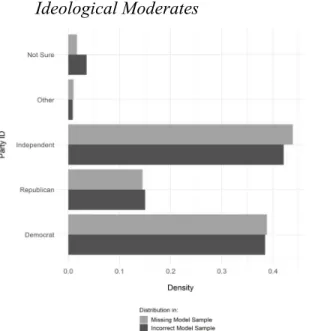
civic knowledge as Republicans; the same was true for having medium civic knowledge, as well as low (109). Instead, it found that the respondent’s ideology was a significant predictor. People who identified farther from the center within their party were more likely to have high civic knowledge (e.g., conservative Republicans were more knowledgeable than moderate or liberal Republicans) (110).
An important note must be made regarding common measures for political knowledge. First, in his book, Brennan raises concerns about the fundamental accuracy of approximations of people’s knowledge levels – not only self-reported ones like in Freiling (2017), but also
calculated ones like those used in Pew (2018b) and this thesis. Naturally, people may simply be wrong about knowing something, as is the concern in Freiling (2017). More critically, on calculated political knowledge measures, such as whether someone correctly identifies the party in control of a legislative chamber, some error can be introduced due to guessing; there is some non-zero, relatively significant change that someone simply guessed the correct answer (Brennan 2016, chapter 2, page 3). This is of concern for this thesis, as the political knowledge measure that was used in analysis is a calculated political awareness measure.
has been found to persist even after controlling for factors such as age, race, education, income, political engagement, and employment (Garand, Cuynan, & Fournet 2004).
One explanation for this persistent effect has been the nature of questions asked. Many authors have found that broad questions about “national-level politics and the rules of the game” favor men (Miller 2018, 177). In a 2011 paper, Kathleen Dolan finds that asking gender-relevant questions about politics, e.g. the percent of women in Congress, leads the long-reported gender differences in political knowledge to essentially “disappear.” Other topics on which women tend to perform equally with or better than men include identifying candidate positions on abortion and naming the head of the local school board (Delli Carpini & Keeter 1996, Shaker 2012).
Miller (2018) references literature providing two theoretical explanations for women’s lower performance on national, institutional questions but higher performance on
gender-relevant or local questions. First, Dolan (2011) found that people are more likely to pay attention to politicians who are descriptively more like them – and because there are far fewer women in national public office than men, women may pay less attention to national politicians, because they relate to them less. Second, Stolle and Gidengil (2010) found that women benefit more frequently from government services and are employed in government more frequently than men, yet questions gauging knowledge of government services are almost never included in traditional political knowledge questionnaires.
expect that these questions may be less gender-biased. Her research finds that there is no statistical difference between the rate at which men and women correctly identify the majority party in the respondent’s home state (Table 3) – a more local identification, like the four personal representation identification questions. This topic is further explored in Chapters Three and Four when this thesis’ specific knowledge measures are created and explored in descriptive analysis.
Fortin-Rittberger (2016) offers an additional step that can be taken to account for some of the gender bias in survey-response based political knowledge scores; her findings suggest that calculating scores as a proportion of correct responses out of only valid responses removes a nontrivial amount of the gender difference in political knowledge (Table 2). Considering respondents’ accuracy only if they affirmatively answer removes a substantial amount of gender’s effect on knowledge, by accounting for the gendered difference in likelihood of guessing versus abstaining from answering (393). Such a metric will be used in this thesis’ analysis. Nonetheless, gender will still be controlled for, because of its effects on social media and on voting, as well as because traditional-type political knowledge questions must be used.
3. Political Participation
The final set of predictors to identify are those of the outcome: voting. This section relies mostly upon the work of the MIT Election Data and Science Lab, which used data from the United States Election Project and the Census Bureau to calculate nationwide 2016 voter turnout by demographic groups. Their analysis begins by touching on over-reporting bias in survey-based voter turnout rates, which is addressed in this thesis as well, in Chapter Three.
with more than a high school degree voted in 2016, while only 44% of people with a high school degree or less did. Another wide gap is found when stratifying by income: people in families with income of more than $50,000 were 69% likely to vote, while people in families with income of less than $50,000 were 50% likely to vote. Age also was a significant predictor of voter
turnout; those aged 60+ voted at a rate of 72%, while those aged 31 to 60 voted 62% of the time and those aged 18 to 30 voted only 44% of the time. Married people voted 18 percentage points more frequently than unmarried people (69% versus 51%) and women voted five percentage points more frequently than men (63% versus 58%). Finally, white people were the most likely racial/ethnic category to vote, at 65%, followed by black people at 60%. Hispanic, Asian-American, and “all other” people voted at roughly 46%. All these turnout rates also varied by state. I speak in more detail about state-by-state turnout in Section 2.A below, but speaking generally, state turnout rates in 2016 ranged from 42% to 74%, with a mean of 61% and a standard deviation of 6%.
4. Putting It All Together
The three previous sections have reviewed literature that describes the individual predictors of each of the three larger concepts at hand in this thesis: social media (news) use, political knowledge, and political participation. This section reviews the existing literature that has connected two or more of those. Much of that work comes, in one way or another, from Homero Gil de Zúñiga of the University of Vienna. After reviewing that literature, the chapter concludes with a summary table of potentially confounding variables in analysis.
participation. Kenski and Stroud (2006) found that internet access and exposure to online
political content were statistically significant, though substantively limited, predictors of political knowledge and participation. In addition, they found that sex, age, race, education, income, and partisanship – both direction and strength – were predictors of both outcomes (knowledge and participation) (Table 3).
Shah, Cho, Eveland, and Kwak (2005) looked at information seeking, which is slightly different from Kenski and Stroud’s exposure. Additionally, while Kenski and Stroud (2006) control for gender, race, education, and income, Shah et al. (2005) do not use any demographic controls in their models. Shah, et al. developed three types of structural equation models, one cross-sectional, one with fixed effects, and one auto-regressive. Because this thesis does not deal with panel data, the cross-sectional model is most comparable and will be the most discussed, though the patterns in Shah et al.’s findings do not differ greatly among the three models (551).
In their model, Shah et al. measure three types of information seeking: searching online, reading the newspaper, and watching TV. They also qualify two types of political expression: “interpersonal political discussion,” i.e. talking about politics with friends, family, neighbors, coworkers, etc., and “interactive civic messaging,” e.g. emailing a politician or writing a letter to the editor (541). Finally, they measure civic participation as self-reported frequency of
volunteering, working on community projects, attending community meetings, or doing otherwise charitable work (540).
the newspaper is found to have a direct effect on civic participation (546). Nonetheless, the indirect effect of online information seeking on civic participation through the two types of political expression remains.
The model structure and findings of Shah et al.’s paper are both very informative for this thesis. Nevertheless, the connections are not perfectly lined up. Given the time-frame of the paper’s analysis, the 2000 election, the types of online activity measured here are starkly different from the online social media news use at hand in this thesis. In 2000, if people wanted information about politics, they truly had to seek it out, which is why Shah et al. term it
“information-seeking” in their paper. That type of behavior is also fairly similar to reading the newspaper, which requires a conscious choice to obtain the information and then be able to read it. The same could be said of watching TV news, though the comparison is less strong.
The social media news use that is being studied in this thesis requires not nearly as much “seeking-out” of the information. People may encounter news items on their social media feeds because they follow an outlet’s page, because a personal connection shared it, or even because it was advertised. The amount of effort required to encounter news on social media in 2016 was very different from the threshold set in Shah et al.’s analysis.
Additionally, the civic participation outcomes in Shah et al.’s paper are truly “civic,” rather than political – i.e., Shah, et al. do not look at voting. Rather, they look at more localized community engagement, like going to meetings and volunteering for nonprofits.
defined as “resources that can be accessed or mobilized through ties in [one’s social] network” (Lin 2008, 51). Online political participation in GZJV (2012) includes making donations, emailing politicians, and subscribing to a political listserv (324). The remaining two outcomes split the civic behaviors used as outcomes in Shah et al. (2005) above: GZJV’s (2012) “civic participation” outcome includes raising charitable moneys, attending neighborhood meetings, and being a conscious consumer, and their “offline political participation” outcome includes voting, putting up signs, and attending a rally (324).
Informing the methodology of this thesis, GZJV (2012) perform four sets of hierarchical regression analyses, one for each set of outcomes. They find that
after controlling for demographic variables, traditional media use offline and online, political constructs (knowledge and efficacy), and frequency and size of political discussion networks, seeking information via social network sites is a positive and significant predictor of people’s social capital and civic and political participatory behaviors, online and offline. (319)
Specifically, they find that getting news from social media was a statistically significant
predictor of offline political participation at the p < 0.001 level. Additionally, GZJV (2012) find that age, education, and getting news from non-social media sources are all also statistically significant predictors of offline political participation.
more intense processing of information may be required for knowledge to be gained. That fact notwithstanding, the effect was still non-trivial, which supports the focus of this thesis.
Jung, Kim, and Gil de Zúñiga (2011) offer a few additional helpful findings for this thesis. They confirmed the causal order of news use political knowledge voting, by running their model with each possible ordering of variables (421). They also hypothesized that “attitude strength” might be a confound that was not included in their analysis (424), which informs the use of party ID and ideology as confounds in this thesis.
Lastly, the measure used for political knowledge by Jung, Kim, and Gil de Zúñiga (2011) dealt with only “general” political knowledge – who is the current Speaker of the House, who is the current British Prime Minister, which state is Sarah Palin the governor of, and so on (418). In light of the discussion in the Political Knowledge section above, this measure may be
problematic for several reasons. In their conclusions, the authors note that other types of knowledge should also be investigated, including candidates’ issue stance knowledge, which “may be more relevant than general political knowledge in an election context” (425). As will be seen in Chapter Three, this thesis uses two measures of knowledge in analysis: “General” and “Personal.” While both types ask respondents to identify the party of something (a legislative chamber or an elected official, respectively), knowledge of one’s own representatives in government (“PersonalKnowledge”) represents a slightly different dimension of political knowledge than the general identification questions used in Jung, Kim, and Gil de Zúñiga (2011). It may also be less subject to the widely-reported on gender bias in national and
measure as a simple sum of correct answers (418), in contrast to this thesis, which calculates knowledge as the proportion of correct answers out of attempted answers.
One variable that was used in Jung, Kim, and Gil de Zúñiga (2011) that is not in this thesis is internal political efficacy. The authors found that, in addition to political knowledge, internal political efficacy was found to be a strong mediator of the relationship between news use and political participation. In other words, based on the authors’ findings, getting news from social media makes people feel more capable of influencing the political process, which leads them to do so (422). The CCES contains no variables that could be used to approximate political efficacy, so unfortunately, it was not considered in analysis.
Finally, another paper co-authored by Homero Gil de Zúñiga investigates the distinction between news consumption and active engagement. Weeks, Ardèvol-Abreu, & Gil de Zúñiga (2017) use the terms “opinion leaders” and “prosumers” to refer to people in their study who actively commented on, forwarded, or created news content on social media. The study focused on those people’s self-perceptions and whether seeing oneself as an “opinion leader” makes one more likely to try to influence others’ politics. They found that people who are more actively engaged with politics on social media do have outsized effects on other people’s political attitudes and behavior, which grants policy relevance to RQ2 (15). That influence was corro-borated by Turcotte et al. (2015), which found that people trusted a news story’s source more when they believed the story had been posted by one of their real-life Facebook friends. The effect was even greater when the participant perceived the friend as an opinion leader.
control variables that should be included in regression analysis. For clarity, I have summarized this chapter’s findings regarding control variables in Table 2 below, which indicates which of the three main variables (social media use, political knowledge, and voting) each potential confound is related to, and which sources in the literature provide evidence of that relationship.
In addition to giving legitimacy to the methods of this thesis in those parts held common, some of the literature cited in this chapter shows the novelty of the methods of this thesis. First and foremost, no paper has looked at social media news use, political knowledge, and voting in the specific context of the 2016 election. Given the nature of that election, there is ample reason to believe that people may have had a different relationship to social media than in previous political contexts. Additionally, the knowledge measure used in this thesis differs from that used in previous work and may be less gender-biased than knowledge measures used in previous work relating social media news use, knowledge, and voting.
Table 2: Summary of Potential Confounding Variables
Characteristic Using Social Media Political Knowledge Likelihood of Voting
Education 1,2,7 5,6,11 7,8,11
Income 1,10 5,11 8,10,11
Region of the US 5
Political Attitudes 10 6,10,11 10,11
Age 2,3,7,10 5,6,11 7,8,10,11
Race 1,2 5,11 8,11
Gender 1,4 5,9,11 8,11
Marital Status 8
Other News Use 7 7 7
State of Residence 5
Methods
Drawing on the theoretical foundations established in the previous chapter, this chapter establishes statistical models that might provide answers to the two research questions of this thesis. The chapter begins by building a causal diagram to relate social media news use, political knowledge, and voting, using the potential confounding variables uncovered in the previous chapter. Then, an overview of the data source is provided, and some of its strengths and limitations are discussed. Next, variables are operationalized, which includes two exploratory factor analyses. Finally, the operationalized variables are combined with the causal diagrams to construct two sets of regression analyses.
1. Causal Diagram
Based on the predicted confounding variables identified in Chapter Two and summarized in Table 2 above, a causal diagram relating social media news content, political knowledge, and likelihood of voting was constructed. That diagram is included as Figure 1 below. Any
characteristic that, based on the literature, was expected to influence two or more of the main variables was included as a potential confound in the graph.
It should be noted that there are many relationships between the confounding variables that have not been included in this diagram, for clarity. For example, age, sex, and race, are all strong predictors of both education and income, and education and income are themselves related as well. If one or more confounding variables did not have a direct effect on the outcome, i.e. did not have an arrow drawn from itself to voting, it would be necessary to chart each of these relationships in order to find and close the correct biasing pathways using Pearl’s backdoor criterion (Pearl 1998, 255-259). However, each confounding variable has, based on the literature, a direct effect on both the treatment and the outcome. Therefore, all confounding variables that can be controlled for will have to be controlled for, making their inter-relationships, for charting
purposes, moot.
Additionally, it should be noted that there are some predicted confounds in this
relationship which cannot be controlled for – most importantly personality. Also omitted from this diagram are predictors which have not been theorized to be confounds – those variables from Table 2 above which are theorized to affect only one of: treatment, mediator, and outcome.
2. The 2016 Cooperative Congressional Election Survey (CCES)
As mentioned previously, this thesis uses data from the 2016 Cooperative Congressional Election Survey (CCES). The CCES is unique among political surveys for several reasons. Chief among them for this thesis is that it asks respondents about their active online news-related activity – whether they read or watch political news content, share political information, put their own opinions out online, and so on. Other surveys, such as the American National Election Survey and ones conducted by the Pew Research Center, are superior on more traditional
questions of media literacy (i.e. access to, frequency of, and attitude towards internet use), but do not include questions relating to active engagement with political news material.
The CCES is a national project, the collaborative product of sixty teams across the country. In 2016, each team surveyed roughly 1,000 people in two waves, pre-election (September 28 to November 7, 2016) and post-election (November 9 to December 14, 2016). Survey respondents were asked questions from three pools, which constitute three tiers of content: Common Content, Group Content, and Team Content. Teams and groups of teams have access to their unique content, while the Common Content is made publicly available through the Harvard Dataverse (Ansolabehere & Schaffner 2017). The Common Content data are the source for this thesis, and they include basic sample identifiers, including weights; demographic
information, including ideology and voter registration status; pre-election questions; post-election questions, including vote-validation data; and contextual data, including candidate and incumbent information.
understanding of YouGov’s privacy policy, which includes anonymization of any individual data provided to clients, such as the researchers behind the CCES (YouGov.com).
To gather the sample, YouGov used a matched random sample methodology for data collection. This method matches individuals in a sampling frame to a researcher-provided target population, using the same theoretical foundations as stratified sampling. First, both the target population and YouGov’s member base are broken into the same mutually exclusive and
exhaustive strata. For the 2016 CCES, over 150,000 YouGov members were pooled to construct these strata. Potential respondents were then recruited out of each YouGov stratum through simple random sampling until the proportion of each sample stratum within the total sample population matched its equivalent’s frequency in the target population (Ansolabehere, Schaffner, & Luks 2017, 12). The sample for the 2016 CCES was later limited again to those respondents who completed both the pre- and post-election waves of questions, after which point weights were applied. The final product is a nationally-representative sample of 64,600 respondents.
YouGov’s online sampling methodology is advantageous because of the large sample size it makes possible. This large sample size enables, among other things, state-level validation of the CCES sample, by comparing CCES two-party vote share predictions to actual state-level results. Graphs comparing the CCES estimate and actual two-party vote share in the presidential, senate, gubernatorial, attorneys general, and secretaries of state elections are included on pages seventeen to twenty-one of the 2016 CCES guidebook. They show that CCES estimates are a very good approximation of actual electoral outcomes, with over 95% confidence of a match between estimate and actual outcome in most cases (Ansolabehere, Schaffner, & Luks 2017, 17).
The main drawback of CCES data is YouGov’s digital sample frame. All survey
meaning the sample is likely to be biased towards people who use social media. The primary authors of the CCES acknowledge this limitation in CCES documentation when enumerating assumptions necessary to confirm the representativeness of the CCES sample (Ansolabehere, Schaffner, & Luks 2017, 12-13).Specifically, they reiterate the “common support” assumption, which holds that the range of values in variables used for sample matching must be plausibly the same for people included in the survey sample as for people not included in the sample frame. Because the survey is executed via computer, this excludes any variable measuring computer use from being a matching variable, because there cannot be anyone in the survey sample who never uses a computer. Because of that fact, it cannot be said with certainty that the survey sample and the target population (the US population, in this case) are the same on such metrics. However, there is nothing that can be done quantitatively to correct for this, and it can only be noted as a limitation.
2 A. Vote Validation in the CCES
A second problem spot – to avoid calling it a limitation – in the CCES is vote validation. Several research teams have independently identified discrepancies relating to validated vote calculations that can be performed using the CCES (Grimmer, et al. 2017; Agadjanian 2018a; Agadjanian 2018b; Ansolabehere & Hersh 2012). The problem is not limited to just the CCES, though; most surveys dealing with voting behavior consistently over-estimate voter turnout rates (Cuevas-Molina 2017, 1). Political scientists have postulated several explanations for this, including sample selection bias, a social-desirability effect, and a combination of the two
there is a societal norm of voting, and people are reluctant to admit to not having done so, even in anonymous survey interviews. These may not only independently bias surveys’ voter turnout metrics, but also interact, according to Bernstein, Chaha, and Montjoy (2001), who predict that “people who are under the most pressure to vote are the ones most likely to misrepresent their behavior when they fail to do so” (24). If people have self-selected into a political survey and therefore care more about politics, but for whatever reason(s) did or could not vote, they may be even more likely to make false claims than someone to whom politics is less important.
Whatever its causes, the effect is “non-trivial” in essentially all national surveys that deal with voting, and must be addressed (Cuevas-Molina 2017, 1). To do so, survey makers now use publicly-available voter registration records and privately-sold voter lists in order to validate people’s reported voting behavior. Before releasing a data set, teams can match as many survey respondents to official voter records as possible, in order to confirm or contradict their self-reported voter registration status and voting history (Ansolabehere & Hersh 2012, 437). More than roughly ten years ago, researchers were limited in the extent to which they could do this, given irregularities in availability and quality of data. The CCES was the first project to perform fifty-state vote validation, in 2012 (439). Historically, even after performing vote validation, the CCES still overestimates voter turnout; Agadjanian (2018b) shows that the CCES overestimated national voter turnout in 2012 and 2014 by 6 and 14 points, respectively. These calculations were performed using CCES’ validated turnout and voting-eligible for highest office turnout from the United States Election Project (Agadjanian 2018b; data available through McDonald n.d.).
altogether; whether someone says they voted is a decent indicator of political interest and using such a measure avoids the risk of creating false-negatives. However, doing so would also hamstring any causal claims that might be made; any findings would not relate to a person’s actual likelihood of voting, but rather only to their likelihood of saying they voted.
Because of that limitation, it was decided that this thesis would use a validated vote measure. Therefore, a choice had to be made between the three validated vote measures outlined by the CCES authors. Those measures make use of information made available by a
collaboration between the CCES team and Catalist, a political data firm. Researchers compared 2016 CCES respondents to a national database of registered voters prepared by Catalist, which resulted in 45,117 (69.84%) of those who completed both waves of the CCES survey being matched to a state’s voter file. 19,483 (30.16%) were not.
The three vote validation measures suggested by the CCES authors are explained in more detail in Table 3. The first method, VV1, maintains the largest sample size, by making a non-voter out of anyone who was not affirmatively matched as a registered 2016 non-voter. This method relies on the accuracy of both government voter file data and CCES survey responses for matching, making its definition of non-voters the least rigorous. While this will unfortunately result in some false-negatives, the CCES authors point out that the most common reason that respondents couldn’t be matched was that they were in fact not registered to vote; rates of self-reported non-registration/non-voting were “much higher” among those not matched to a voter file than among those matched (Ansolabehere, Schaffner, & Luks 2017, 126).
significantly (dropping 30% of the original data set), though it has the benefit of reduced likelihood of false negatives.
Finally, while VV1 and VV2 employed in their classifications only the variables for being matched to a voter registration and for having cast a verified 2016 vote, VV3 also employs self-reported registration and voting behavior. Among respondents who could not be matched to a voter file, VV3 takes self-reported non-registered and/or non-voting people at their word. The CCES authors justify this assumption on the grounds that “self-reported non-voters are honest about their non-participation because there is no incentive to go against the democratic norm of participation” (126 – emphasis added).
Table 3: Defining Three Validated Voter-Turnout Measures
Measure Voters Non-Voters Treated as Missing
VV1
*Matched to voter registration and vote confirmed as cast
*Matched to voter registration and vote confirmed as not-cast *Not matched to any voter registration
None
VV2
*Matched to voter registration and vote confirmed as cast
*Matched to voter registration and vote confirmed as not-cast
*Not matched to any voter registration
VV3
*Matched to voter registration and vote confirmed as cast
*Matched to voter registration and vote confirmed as not-cast *Not matched to any voter registration and self-reported not being registered to vote *Not matched to any voter registration and self-reported not casting a vote
*Not matched to any voter registration and self-reported not having cast a vote
Each validation method has its advantages and disadvantages, with none being clearly strictly-dominated or dominant on qualitative considerations. Empirics help to decide which measure to use in analysis. Table 4 compares state-level CCES predicted turnout using each of the three measures to actual turnout. Comparisons are made to two different statistics for “actual turnout” from the United States Election Project: turnout among the voting-age population (VAP) and among the voting-eligible population (VEP).
Both the VAP and VEP comparisons are included, for separate purposes: Alexander Agadjanian (2018b) used the VEP in his comparisons, but VAP turnout is a better analogue for some estimates of CCES turnout, when respondents are not limited to eligible voters. Whether the CCES sample is more like the voting eligible or voting age population changes depending on the VV method used. When using VV1, the sample is more similar to the VAP, because non-matched respondents are considered simply non-voters, rather than excluded as missing; voting non-eligible people are still included as the sample, as non-voters, rather than excluded
completely. For VV2, the sample is more like VEP, because the sample is limited only to matched registrants, meaning that no voting-non-eligible people can be in the sample. For VV3, neither VAP nor VEP is a great match, because VV3 uses includes some non-matched
respondents in the sample, but not all.
Table 4: Selecting a Validated Voter-Turnout Measure
Turnout Measure: VV1 VV2 VV3 VV1 VV2 VV3
Compared to
Turnout Among: Voting Age Population Voting Eligible Population
Average Percent Error (%) 8.38 42.15 28.41 9.31 32.07 19.36
Average Bias (%-Pt. Diff) 0.91 22.98 15.41 -3.25 18.83 11.26
Average |Bias| 6.65 31.05 21.49 0.56 24.96 15.40
SOURCE: Actual Turnout Data from McDonald (n.d.): www.electproject.org/2016g
Agadjanian’s (2018b) findings also appear to support the selection of VV1 as the voter-turnout measure of choice. Agadjanian’s figures report that 2016 CCES state-level voter-turnout estimates are off from VEP turnout by an average of -4 percentage points. This is quite close to the -3.25 average bias figure that was calculated for VV1 as compared to the same actual turnout measure (VEP). The two average bias estimates are not exactly equal, which is of some concern, but it may be due to a difference between the 2016-only CCES data set (used in this thesis’ analysis) and the 2006-2016 CCES Cumulative File (used in Agadjanian’s analysis).
3. Modeling Social Media Behavior
The next step to prepare the CCES data for analysis was to devise measures for the two types of news-related social media behavior described in RQ1 and RQ2: consumption and active engagement. To create those measures, explanatory factor analysis (EFA) is performed on five variables from the CCES.
As introduced above, the CCES is unique in that it asks respondents above their active social media posting, not just their social media use. Also distinctive about these questions is that they ask the Yes/No question of whether respondents engaged in a given activity in the last twenty-four hours, rather than how frequently they may have done so over a given period of
time, such as the last week. Framing questions this way should increase the accuracy of the measure. People are notoriously poor estimators, including when it comes to their own behavior (Brennan 2016). Asking respondents to remember only whether they did something at all over the last twenty-four hours of their lives, rather than summarize the frequency of doing so over the last week, or month, theoretically increases the odds that they provide an accurate answer.
All five questions used to create social media scores were asked in the pre-election wave. Respondents were first asked whether they had used social media in the past twenty-four hours. 19,286 respondents had not. The 45,314 respondents that answered in the affirmative were asked a follow-up question which asked whether they did each of the following on social media in the last twenty-four hours:
1. “Posted a story, photo, video or link about politics” 2. “Posted a comment about politics”
3. “Read a story or watched a video about politics” 4. “Followed a political event”
Given the five variables, the total number of possible response patterns is 32. The relatively small size of this set of possible response patterns (Bartholomew, Knott, & Moustaki 2011, 84) allows it to be displayed as a frequency distribution (included in the Appendix as Table 10). Brief examination of this distribution allows some insights. The most frequent
response pattern, at 22.69% of social media users, is a respondent having read or watched a story about politics in the past twenty-four hours but not having engaged in any of the remaining four activities. The next two most frequent patterns are markedly less than the most frequent
response. These second and third-most frequent response patterns are also the two extremes: having engaged in none of the activities in the past twenty-four hours and having engaged in all of them. Having engaged in none of the activities is roughly 5 percentage points less frequent than the most frequent pattern, coming in at 17.45% of social media users, and the jump from none to all is even more drastic, with only 10% of social media users engaging in all six activities (a difference of roughly 7.5 percentage points).
With an understanding of the pattern of people’s responses, the next step was to attempt to analytically differentiate between the two types of social media news use, consumption and active engagement. Factor analysis allows that difference to be teased out specifically within the analytical sample of this thesis.
EFA works by testing a range of hypotheses regarding the relationships between the observed variables, narrowing the set of hypothetical relationships to find which variables tend to “go together” (Yong & Pearce 2013, 80). The final output of EFA is the smallest set of factors that accounts for the highest amount of correlation amongst the observed variables (80). Ideally, each variable will be highly correlated with one factor and not strongly correlated with any other. The correlation of each variable with each factor is called a “loading,” and the table of each variable’s loading onto each factor is called a “pattern matrix.” Hair et al. (1998) provide thresholds for practical significance of factor loadings: ≥ 0.3 = “minimal,” ≥ 0.4 = “more important”, and ≥ 0.5 = “practically significant” (111). The “communality” of a variable in a factor analysis is the sum of its squared loadings, and can be interpreted as the proportion of total variation in that variable that is explained by the factors.
The factor analysis below was performed in Stata/IC 15.1, as was all other analysis. Stata’s factor command was used to perform EFA, using the iterated principal-factor option (IPF) based on the recommendation of Habing (2003). Whereas other methods for fitting factor analysis models use the same initial estimate of each variable’s communality throughout each successive attempted model fit, the iterated principal factor method recalculates the
communalities with each new fitted model (Habing 2003, 5). Habing (2003) recommends IPF so long as the final model has neither impossible communalities (greater than one) nor negative error variances (5). As is seen below, neither is the case in this model.
al.’s (1998) thresholds, these loadings are of less than even “minimal” practical significance. On those grounds, further analysis is limited to only the first two factors.
After limiting the EFA to only two factors, Stata returns an improved pattern matrix with more-significant loadings (included in the Appendix as Table 12). Posting, commenting,
forwarding, and following all have practically significant loadings onto at least one factor, and reading/watching is slightly more than minimally significant. However, another potential
problem remains: multiple variables load relatively-significantly onto more than one factor. This will make interpretation of the factors more difficult, and according to Habing (2003), should be avoided if possible.
To correct this, the factors can be rotated. Dr. Maike Rahn of TheAnalysisFactor.com provides a very intuitive explanation of factor rotation. As Dr. Rahn describes it, the two factors are axes along which each variable is positioned. When Stata conducts the initial EFA, it isolates the first factor (axis), holds that constant, then finds the second. Once these two factors (axes) have been found, however, they do not always result in the best possible fit of the data. Rotating the axes can make them fit the variables better. A side-effect of rotation is that it ideally aligns each variable primarily with only one factor, thereby making the factors more easily
interpretable.