TRANSACTIONS ON ENVIRONMENT AND ELECTRICAL ENGINEERING ISSN 2450-5730 Vol 3, No 1 (2019) ©Vishnu Sidaarth Suresh
Abstract—Load flow studies are carried out in order to find a steady state solution of a power system network. It is done to continuously monitor the system and decide upon future expansion of the system. The parameters of the system monitored are voltage magnitude, voltage angle, active and reactive power. This paper presents techniques used in order to obtain such parameters for a standard IEEE – 30 bus and IEEE-57 bus network and makes a comparison into the differences with regard to computational time and performance of each solver. The objective being to first understand the working of each solver and then come to conclusions regarding the best one keeping in mind the network size and complexity so that it can extended to bigger networks for analysis. The methods are evaluated in this study using Matpower which is a tool meant for academical purposes and not intended for on-line use.
Index Terms—Load flow, IEEE 30 bus, IEEE 57 bus Numerical methods.
I. INTRODUCTION
HE load flow problem is an important tool for the operation and control of power systems. It gives the system operator information regarding active power, reactive power demand and consumption, voltage magnitude and voltage angle at every bus within the system which enables the operator to execute an appropriate schedule for dispatch of power. This information is also useful while planning expansion of power systems and helps maintain power system stability [1].
There are many techniques in-order to address the load flow problem [2-4], the techniques are numerical methods that are used to solve non-linear equations in order to obtain the steady state parameters of the system. In [5] network design and load flow analysis were carried out using ETAP and the resulting conclusions were taken as considerations for future expansion of power systems. In [6] load flow studies are performed using Newton-Raphson and decoupled load flow methods and a comparison is made amongst systems with and without unified power system controllers. [7] used ‘Distflow’ for comparison of different numerical methods based solvers for the load flow problem. [8] uses a power system analysis toolbox called ‘Mipower’ to study the performance of Gauss-Seidel method on an IEEE-3 Bus system. [9] presents a unique
Vishnu Suresh, PhD candidate – Wroclaw University of Science and Technology, Faculty of Electrical Engineering, Wybrzeze Wyspianskiego 27,50-370 Wroclaw, E-mail: vishnu.suresh@pwr.edu.pl.
.
power flow iterative algorithm and it is applied to a modified IEEE – 30 consisting of two wind farms in order to validate the model. [10] provides a novel method called Nonsy load flow in which the study has conducted load flow analysis using data that is unsynchronized and is obtained from diesel generators and the main substation in their network. Once this data is obtained other parameters of the network are solved using backward/forward sweep methods. This study makes a comparison of the performance of the methods using Matpower applied to two standard IEEE test bus cases.
Matpower is a useful toolbox in Matlab to solve the load flow problem, it is developed by the power system engineering research center at Cornell University [4]. It is intended for academical use and understanding the different methods for solving load flow problems.
In this paper we compare solving of the load flow problem for a standard IEEE-30 and 57 bus test cases using Gauss-Seidel, Newton-Raphson and Fast decoupled load flow (FDLF) techniques in Matpower and come to conclusions regarding the characteristics of each method. The reason for taking two test cases is to understand how the performance of the solvers varies with increased network size and complexity. Moreover, such a comparison would enable the choosing an appropriate solver for analysis of city sized networks.
The version of Matpower used is 7.0b1, installed in Matlab 2018b in a Windows 10 64-bit system with an i5 core processor. The computational time in this study indicates the overall time take to obtain the solution whereas performance of each solver indicates the time taken per iteration and computational burden refers to the memory that is needed to run each solver. Convergence is defined as a property of a solver to reach the solution vector, It represents the ability of a function to approach a limit as terms in the series increases.
The IEEE-30 bus test case system has a total of 6 generators, 24 loads, transmission lines at 1kV, 11kV, 33kV and 132kV along with capacitor banks at certain buses for reactive power compensation. The IEEE-57 bus test case system has a total of 7 generators, 50 loads, transmission lines along with capacitor banks at certain buses for reactive power compensation. The test systems serve as a representative model to carry out power system studies and load flow analysis. The load flow problem involves solving for 4 parameters at every bus: active power(Pi), reactive power (Qi), voltage magnitude (Vi) and voltage angle (i ) where i =
1,2,…..,n denotes the number of buses and if there are n buses then the total number of variables to be ascertained are 4n, but power flow studies usually assume bus types which usually
Comparison of Solvers Performance for Load
Flow Analysis
Vishnu Suresh
keeps 2 out of 4 variables as constants, thereby reducing the number of variables to be solved to 2n. The bus types are summarized below [2, 3]:
PQ bus/Load bus: In this type of bus the total active power (Pi) and reactive power (Qi) at the bus are known, and is calculated as a difference between the active and reactive power injected and consumed in a bus. Hence, the variables to be determined include voltage magnitude (Vi) and voltage angle (i).
PV bus/Voltage controlled bus/Generator bus: This type of bus is usually preferred for power generating sources. Here, the total active power injected and consumed is known (Pi) and the voltage magnitude is maintained at a particular value by means of reactive power injection. Hence, the unknown variables are total reactive power at the bus (Qi) and voltage angle (i). Swing bus/Slack bus/ Reference bus: In this type of bus
the voltage magnitude (Vi) and the voltage angle (i) are known and the active power (Pi) and reactive power (Qi) are unknown. The slack bus is in-fact a fictitious concept that is created by a power system analyst in order to study the system [2]. In any load flow study, the total active and reactive power (complex power) at every bus is not known since the net complex power flow within the system is unknown including the total loses along transmission lines. Therefore, it is a convention to choose the largest generator in a system to be the slack bus as it is understood that it is capable of producing active and reactive power according to the needs of the system. There is usually only one such bus chosen in a system as a reference.
In the IEEE test bus cases, the largest generator is chosen as the slack bus and the other sources are chosen as PV buses whereas the loads are modeled as load buses. Once the buses are decided the equations to solve are (1). 𝑃𝑖= |𝑉𝑖| ∑𝑛𝑘=1|𝑉𝑘||𝑌𝑖𝑘|cos(𝜃𝑖𝑘+𝑘−𝑖) (1)
𝑄𝑖= −|𝑉𝑖| ∑𝑛𝑘=1|𝑉𝑘||𝑌𝑖𝑘|sin(𝜃𝑖𝑘+𝑘−𝑖) (2)
Where, i = 1,2,…..,n. Yik – represents self and mutual admittances, between buses i and k and forms the bus admittance matrix Ybus that is crucial to obtain the load flow solution.
In order for static load flow equations to match reality as close as possible it is important to incorporate limits pertaining to all components in the network. The constraints are described as follows:
Voltage magnitude constraints
|𝑉𝑖|𝑚𝑖𝑛≤ |𝑉𝑖| ≤ |𝑉𝑖|𝑚𝑎𝑥 (3)
Voltage angle constraints
|𝑖— 𝑘| ≤|𝑖— 𝑘|
𝑚𝑎𝑥 (4)
This difference with regard to difference of angle during transfer of power between buses i and k is important for system stability.
Constraints of sources to generate active and reactive power
(𝑃𝑔𝑖)𝑚𝑖𝑛 ≤ 𝑃𝑖 ≤ (𝑃𝑔𝑖)𝑚𝑎𝑥 (5)
(𝑄𝑔𝑖)𝑚𝑖𝑛 ≤ 𝑄𝑖 ≤ (𝑄𝑔𝑖)𝑚𝑎𝑥 (6) Pgi and Qgi are the active and reactive power generated at bus i
II. NUMERICAL SOLVERS
A. Gauss-Seidel method
This method is used to solve a set of non-linear algebraic equations. It is an iterative method and begins with an assumption of a solution vector. The assumption is made with regard to practical considerations. Revised value of a variable is obtained by substituting in one of the equations in (1) the remaining present variables of the solution vector. Then the solution vector is immediately updated with this new revised variable. This process is done for all variables in the solution vector in one iteration. The iterations continue until a certain degree of accuracy of the solution vector is obtained. The Gauss-Seidel method is very simple in terms of its usage to solve non-linear equations, also it is not necessary to store data from previous iterations to go to the next iteration. On the other hand, this method is very sensitive to the initial assumption of the solution vector, hence the speed of convergence depends on the closeness of the solution vector to the actual solution. In certain cases when the assumption is highly inaccurate the method might fail to converge [2, 3].
The application of this method to the power system is as follows:
1. First, the load demand (Pdiand Qdi) are obtained at all buses, then keeping relevant constraints in mind the active and reactive power generations (Pgi and Qgi) are allocated at all generating stations and since the largest generating station is kept as a reference bus the active and reactive power generation at this bus is allowed to change during the iterations.
2. The bus admittance matrix Ybus is assembled with the available line and shunt admittance data
3. To begin the iterative process a flat voltage start is assumed and all buses are set to a voltage magnitude and angle of 10o
. Then the voltages at every bus is recalculate by a rearranged version of equation (1) and the iterations continue until an acceptable accuracy is obtained.
𝑣𝑖𝑝+1− 𝑣𝑖𝑝< ℇ
4. Once the voltage values of all buses are known then active and reactive power at the slack bus is obtained. 5. The last step of the process involves calculating the
losses of the system using the line and shunt admittance data along with the known voltage values. These steps describe the method to obtain all parameters for PQ buses since it begins with an assumption of active and reactive power demand and consumption at every bus. For PV buses the iterative method is different with regard to the assumptions made at the beginning of the iterative process, the detailed procedure is described in [3].
B. Newton-Raphson method
This is a powerful tool for solving a set of non-linear equations, the advantages of this method are that it is not sensitive to the assumption of the solution vector made. The
solution in this case converges in most cases as compared to the Gauss-Seidel method and it is done in a fewer number of iterations. The drawback of this method is increased computational burden and the need of additional storage space since it involves calculation of Jacobian matrices and storage of values of previous iterations.
At any iteration, the function is approximated by a tangent hyperplane and the problem is linearized into a Jacobian-matrix equation [3]. The Jacobian Jacobian-matrix consists of slopes of the tangent hyperplanes.
F(X) =—J. ΔX (7) The problem is solved for the correction ΔX - the correction solved is then added to the previous value of X, so the new updated value is closer to the solution and this iteration process continues until an acceptable accuracy is obtained and the correction values in subsequent iterations are very small.
The application of this method to the power system will be as follows:
1. For a PQ bus for which the values of active and reactive power are known (Pi and Qi), an initial assumption of the solution for Vi and i is made. Substituting these values in equation (1) the calculated values for Pi and Qi are obtained then the corrected values are calculated.
𝛥𝑃𝑖= 𝑃𝑠𝑝𝑒𝑐𝑖𝑓𝑖𝑒𝑑−𝑃𝑐𝑎𝑙𝑐𝑢𝑙𝑎𝑡𝑒𝑑 (8)
𝛥𝑄𝑖 = 𝑄𝑠𝑝𝑒𝑐𝑖𝑓𝑖𝑒𝑑− 𝑄𝑐𝑎𝑙𝑐𝑢𝑙𝑎𝑡𝑒𝑑 (9)
These values ΔPi and ΔQi correspond to F(X) in (6) and the corrected values for Viand i can be obtained by solving (6).
2. At the slack bus the values of voltage magnitude and angle Vi and i is fixed. Hence, there would be no equations pertaining to the slack bus in the Jacobian. 3. Once the corrected values ΔViand Δi are obtained, the
next iteration is carried out by adding these corrected values to the previous values of Viand iand step 1 is repeated. This process continues until the corrected values are very small pertaining to an accuracy that is acceptable.
4. PV buses have constant voltage magnitude and active power at every bus and the iterative process is carried out to obtain values for reactive power and voltage angle.
C. Fast decoupled load flow methods.
In transmission systems there is always an interdependence between the voltage angle and active power (-P) and between voltage magnitude and reactive power (V-Q). Hence, the coupling amongst -P and V-Q is weak and this can be exploited in order to make the load flow problem simpler and reduce the computational burden on processing software. This can be done by solving the -P and V-Q problems separately, that is to have two small submatrices for the variables and it is the basis for the decoupled load flow methods. The Jacobian that is formulated in the Newton-Raphson method as mentioned above is simplified by eliminating the elements with weak coupling and it is usually about half of the elements that are eliminated in this manner. This could affect the true convergence of the solution but there is a trade-off between
solution accuracy and reduced computational burden which is acceptable [2, 3].
III. LOAD FLOW ANALYSIS
Load flow analysis will be carried out for all three methods mentioned above on IEEE-30 bus and IEEE-57 bus test cases and the results of each will be discussed in-order to understand the advantages and disadvantages of both.
A. IEEE-30 bus
The summary of load flow analysis of the ieee-30 bus test case, including the total amount of active and reactive power generated, consumed and line losses using Gauss-Seidel, Newton-Raphson and FDLF methods are presented in Figures 1-3 respectively. The Gauss-Seidel method was able to arrive at the solution in 492 iterations and 0.45 seconds.
The Newton-Raphson method was able to arrive at the solution in 2 iterations and 0.14 seconds.
The FDLF method was able to arrive at the solution in 7 P-iterations and 6 Q-P-iterations with a total of 13 P-iterations and in 0.16 seconds. This method takes advantage of the weak coupling between -P and V-Q, hence the equations for both set of variables are solved separately and the number of iterations for the solution also differ.
Figure 1. System summary and load flow analysis using Gauss – Seidel numerical method.
Figure 2. System summary and load flow analysis using Newton-Raphson numerical method
Figure 3. System summary and load flow analysis using Fast decoupled load flow method
B. IEEE-57 bus
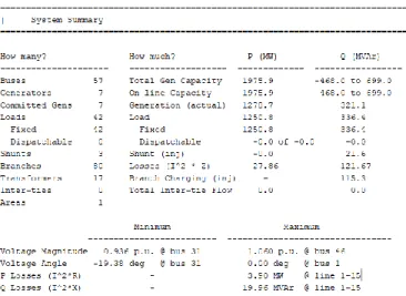
To study the effects of increasing the network size on the performance of numerical solvers, the IEEE-57 bus test case is used and the results are compared with those obtained from the IEEE-30 bus test case. Figures 4-6 represent load flow summary, including the total amount of active and reactive power generated, consumed and line losses using the all 3 methods respectively. The Gauss-Seidel method was able to arrive at the solution in 518 iterations and 0.59 seconds
Figure 4. System summary and load flow analysis using Gauss – Seidel numerical method
Figure 5. System summary and load flow analysis using Newton-Raphson method
Figure 6. System summary and load flow analysis using Fast decoupled load flow method.
The Newton-Raphson method was able to arrive at the solution in 3 iterations and 0.15 seconds.
The FDLF method was able to arrive at the solution in 7 P-iterations and 7 Q-P-iterations with a total of 14 P-iterations and in 0.17 seconds. This method takes advantage of the weak coupling between -P and V-Q, hence the equations for both set of variables are solved separately and the number of iterations for the solution also differ.
C. Convergence of methods
Figure 7. Convergence of Gauss-Seidel method (IEEE-30 bus) Figure 7 describes the convergence of the Gauss-Seidel method (IEEE-30 bus) and in-comparison with Figure 8 it can be inferred that the slope of convergence is quite gradual in this method and the number of iterations are much higher when compared to the Newton-Raphson and FDLF methods (IEEE – 30 bus) as seen in Figure 8. Figure 8 which describes the convergence of Newton-Raphson and FDLF methods, it can be seen that the Newton-Raphson method takes lesser number of iterations, and from Figure 3 the time taken by the FDLF method is 0.16 seconds compared to 0.14 seconds for the Newton-Raphson method from Figure 2, hence it can be concluded that the per iteration is much higher in the Newton-Raphson method when compared to the FDLF method. This is because the assumptions taken in the FDLF method reduce the computational burden hence accelerating the iterative process. It should also be noted that there is no significant improvement in the overall time taken for the load flow analysis between Newton -Raphson and FDLF methods.
Figure 8. Convergence of Newton-Raphson and FDLF method (IEEE-30 bus)
Figure 9 represents the convergence of the Gauss-Seidel method (IEEE-57 bus) to the solution. It can be noticed that the convergence is gradual and it takes a total of 518 iterations for the method to finish. Figure 10 represents the convergence of the Newton-Raphson and FDLF (IEEE – 57 bus) methods. It can be noticed that the convergence in Figure 10 is much steeper and the solution is obtained in 3 iterations for the Newton-Raphson method and 14 iterations (7 – P iterations and 7 – Q iterations) for the FDLF method.
Figure 9. Convergence of Gauss-Seidel method (IEEE-57 bus)
Figure 10. Convergence of Newton-Raphson and FDLF method (IEEE-57 bus)
IV. CONCLUSIONS
A. Results
TABLE I
LOAD FLOW RESULTS FOR IEEE – 30 BUS Characteristics Gauss-Seidel
Newton-Raphson
FDLF Iterations 492 2 7 P-iterations
6 Q-iterations Total – 13
Time 0.45 0.14 0.16
Time/iteration 0.0009 0.07 0.0114 Convergence Gradual Steep Steep Computational
burden
Low High Higher than Gauss-Seidel,
Lower than Newton- Raphson
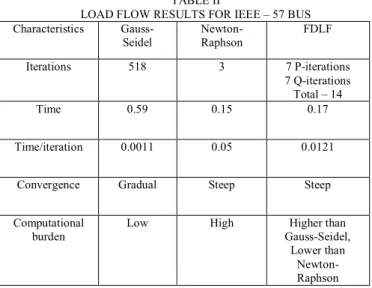
TABLE II
LOAD FLOW RESULTS FOR IEEE – 57 BUS Characteristics
Gauss-Seidel
Newton-Raphson
FDLF Iterations 518 3 7 P-iterations
7 Q-iterations Total – 14
Time 0.59 0.15 0.17
Time/iteration 0.0011 0.05 0.0121 Convergence Gradual Steep Steep Computational
burden Low High Gauss-Seidel, Higher than Lower than
Newton- Raphson
B. Discussions
The comparison of different methods to solve the load flow problem yields the following results, the Gauss-Seidel method takes less time to perform one iteration when compared to the Newton-Raphson method, this is because of the fewer number of arithmetic operations involved in completing an iteration, as the calculation of the Jacobian which is an inherent part of the calculations for the Newton- Raphson method. The Newton-Raphson method has a faster rate of convergence because of its quadratic convergence characteristics. The technique is said to ‘home-in’ to the solution.
For the Gauss-Seidel method the number of iterations increase with the network size i.e. higher the number of buses in the network, the longer it takes for the method to find a solution, this evident from the fact that it takes 518 iterations and 0.59 seconds for the IEEE-57 bus test case to find a solution compared to 492 iterations and 0.45 seconds for the IEEE-30 bus test case. The relationship is not as proportional in the Newton-Raphson method as the time taken for the IEEE-57 test bus case with this method is 0.15 seconds and 3 iterations whereas for the IEEE-30 bus case it is 0.14 seconds and 2 iterations representing only a marginal increase in the computational time. This conclusion holds also for bigger networks with a much higher number of buses [2,3].
The Gauss-Seidel method is relatively easier to implement and does not require a lot of memory, whereas the Newton-Raphson method is complex to implement and does require higher memory and processing capacity.
The Gauss-Seidel method is very sensitive to the selection of the slack bus, In some cases the method is also known to not converge to a solution hence, making the first step of choosing a solution vector very crucial. Inversely, the Newton-Raphson method is not so sensitive to the selection of the slack bus and almost always converges to a solution.
The FDLF method in both cases (IEEE – 30 and 57 bus test cases) takes more iterations and more time to arrive at the solution. It is important to remember that the FDLF method takes into account certain assumptions while searching for the solution making it as fast as the Newton-Raphson method with the advantage of reduced computational needs such as memory and processing capability.
It can be hence concluded that both Newton-Raphson and FDLF methods are efficient and can be extended to bigger and more complex networks but the computational advantage that the FDLF method provides can lead to cost savings. Therefore, the selection of a methods depends on the overall finances involved in solving load flow issues along with speed and accuracy.
Therefore, this paper has described and compared the application of 3 methods in solving the load flow problem for 2 standard IEEE bus test cases and conclusions arrived at commensurate with the objective.
Future study in this regard is to extend the analysis to networks containing renewable energy sources that are unpredictable in their output which makes the load flow problem more complicated and to include time series analysis. The methods can also be executed on other tools and make a comparison as to which tools are most efficient for performing load flow analysis
REFERENCES
[1] Afolabi, O. A., Ali, W. H., Cofie, P., Fuller, J., Obiomon, P., & Kolawole, E. S. (2015). Analysis of the Load Flow Problem in Power System Planning Studies. Energy and Power Engineering, (7), 509–523. https://doi.org/10.4236/epe.2015.710048
[2] Stott, B. (1974). Review of Load-Flow Calculation Methods. Proceedings of the IEEE, 62(7), 916–929. https://doi.org/10.1109/PROC.1974.9544G. O. Young, “Synthetic structure of industrial plastics,” in Plastics, 2nd ed., vol. 3, J. Peters, Ed. New York: McGraw-Hill, 1964, pp. 15–64.
[3] D. P. Kothari and I. J. Nagrath, “Power System Engineering,” 2nd Edition, Tata McGraw Hill, New Delhi, 2007.
[4] R. D. Zimmerman, C. E. Murillo-Sanchez, and R. J. Thomas, \Matpower: Steady- State Operations, Planning and Analysis Tools for Power Systems Research and Education," Power Systems, IEEE Transactions on, vol. 26, no. 1, pp. 12{19, Feb. 2011. DOI: 10.1109/TPWRS.2010.2051168
[5] Prabhu, J. A. X., Sharma, S., Nataraj, M., & Tripathi, D. P. (2016). Design of electrical system based on load flow analysis using ETAP for IEC projects. 2016 IEEE 6th International Conference on Power Systems, ICPS 2016, 1–6. https://doi.org/10.1109/ICPES.2016.7584103. [6] Model, U. M. (2000). Power Flow Analysis of Power System With Upfc, 00(c), 2–5. Dept. of Electric Power & Automation Engineering Tianjin University, Tianjin (300072)
[7] G.M. Gilbert, D.E. Bouchard, A. Y. C. (2010). Comparison of load. International Journal of Engineering and Advanced Technology, 850– 853. Department of Electrical and Computer Engineering Royal Military College of Canada Kingston, Ontario
[8] Kaur, S., Singh, A., & Khela, R. S. (2015). Load Flow Analysis of IEEE-3 bus system by using Mipower Software. International Journal of Engineering Research & Technology (IJERT), 4(03), 9–16.
[9] Phan, T. T., Nguyen, V. L., Hossain, M. J., To, A. N., & Tran, H. T. (2016). An unified iterative algorithm for load flow analysis of power system including wind farms. In L-S. Lê, T. K. Dang, J. Küng, N. Thoai, & R. Wagner (Eds.), 2016 International Conference on Advanced Computing and Applications ACOMP 2016: proceedings (pp. 105-112). Piscataway, NJ: Institute of Electrical and Electronics Engineers (IEEE). https://doi.org/10.1109/ACOMP.2016.024
[10] Bahmanyar, A., Estebsari, A., Bahmanyar, A., & Bompard, E. (2020). Nonsy Load Flow : Smart Grid Load Flow Using Non-Synchronized Measurements. 2017 IEEE International Conference on Environment and Electrical Engineering and 2017 IEEE Industrial and Commercial Power Systems Europe (EEEIC / I&CPS Europe), (646568), 1–5. https://doi.org/10.1109/EEEIC.2017.7977509