Multi-Objective Optimization of Green Supply Chain Network Designs for Transportation Mode Selection

Sharif University of Technology

Transactions E: Industrial Engineering www.scientiairanica.com

Multi-objective optimization of green supply chain

network designs for transportation mode selection

D.-C. Gong

_{, P.-S. Chen}

_{and T.-Y. Lu}

a. Department of Industrial and Business Management, Chang Gung University, Guishan District, Taoyuan City, 333, Taiwan, ROC.

b. Department of Industrial and Systems Engineering, Chung Yuan Christian University, Chung Li District, Taoyuan City, 320, Taiwan, ROC.

Received 10 November 2015; received in revised form 5 October 2016; accepted 29 October 2016

KEYWORDS Supply chain network design;

Green supply chain; Transportation mode; Multi-objective optimization.

Abstract. This research considers both cost and environmental protection to design a multi-objective optimization model. With multi-period customer demands, the model can solve a multi-plant resource allocation and production planning problem by focusing the decisions on supplier selection, facility selection, production batches, transportation mode selection, and distribution of the materials and commodities of a green supply network. In this paper, four transportation modes, namely, road, rail, air, and sea, have their corresponding transportation time, costs, and CO2 emissions. Based on multiple planning

periods, this research calculates the minimal total cost and total CO2 emissions based

on production and transportation capacity. Using numerical analyses, the results show that, when the budget is sucient, only production capabilities with = 1:5 and 2.0 are benecial for improving environmental protection; carbon dioxide emissions of both production capacities are not signicantly dierent. Furthermore, when the production batch size increases, total cost increases. Regarding transportation capacity, the results show that, when the budget is sucient, increasing transportation quantity limits will be slightly benecial for improving environmental protection.

© 2017 Sharif University of Technology. All rights reserved.

1. Introduction

Global climate change has become a key topic and international trends have shifted toward increased reg-ulation of greenhouse gas emissions. In addition, eco-nomic globalization has linked the environment closely

1. Supply Chain Division, Chang Gung Memorial Hospital-Linkou, Guishan District, Taoyuan City, 333, Taiwan, ROC

*. Corresponding author. Tel.: (886) 32654410; Fax: (886) 32654499

E-mail addresses: gongdc@mail.cgu.edu.tw (D.-C. Gong); pingshun@cycu.edu.tw (P.-S. Chen); zey.liu@gmail.com (T.-Y. Lu)

doi: 10.24200/sci.2017.4403

to global supply chains. Production activities consume tremendous energy, with the manufacturing and trans-portation industries producing the most carbon diox-ide. Thus, corporations that wish to reduce greenhouse gas emissions in their supply chain should begin with their manufacturing and transportation methods [1].

Beamon [2] dened a supply chain as \the network structure of raw material suppliers, manufacturers, wholesalers, retailers, and end customers involved in the production and transportation of a product formed through integration." To enable eective, long-term operations of the entire supply chain, the design of Supply Chain Management (SCM) networks frequently involves strategic policy concerns that encompass ma-terial sources, plant location selections, plant produc-tion capabilities, and inventory management [3]. SCM

networks also involve the selection of transportation routes, which include raw material supply and trans-portation modes that begin at the supply end and nish with the customers [4-6]. Melo et al. [7] divided SCM network design according to the nature of product demand and supply chain complexity into the following four categories: (a) single-stage or multi-stage supply chains; (b) single-product or multi-product supply chains; (c) single-period or multi-period planning; and (d) xed demand or random demand.

Since 2000, SCM research topics have shifted toward multiple products. Rizk et al. [8] examined the dynamic production and transportation problems in-volving multiple products using a single plant location and distribution center to plan production, transporta-tion, and inventory within a limited cycle. The study contained dierent transportation times and costs to solve the values of decision variables with the objective of minimizing cost. Similar studies include Nishi et al. [9] who used Lagrangian decomposition to solve the multi-stage supply network problems of a single plant with multiple products. Kanyalkar and Adil [10] incor-porated production capabilities and limited inventory space, and applied the heuristic method to maximize target prots. Hugo and Pistikopoulos [11] developed a multi-supplier and multi-plant production transporta-tion network model of productransporta-tion investment choices to select production technology investments that achieved the target net present value and carbon emission minimization.

In practice, product movement cannot be achieved by relying on only one transportation mode. Suitable transportation modes must be selected on the basis of product weight, dimensions, product value, and urgency. Das and Sengupta [12] investigated numerous uncertain factors involved in international corporation strategies and operations, including investment in raw materials, transit costs, duties, and changes in demand and transportation time. This two-stage mathematical solution model used prot maximization as the strate-gic dimension target to obtain supply chain network decisions (e.g., whether plants should enter production, product types, and quantity produced by each plant). The results were then used in the operations dimension to explore cost minimization inventory strategies when transportation times uctuated.

Sadjady and Davoudpour [13] discussed single-phase requirements and network planning of multiple products, and then used cost minimization to deter-mine the location of plants and distribution ware-houses and transportation modes. The Mixed Inte-ger Programming (MIP) model proposed by Sadjady and Davoudpour incorporated transportation times, carrying costs, and facility setup costs of various transportation modes and used Lagrangian relaxation to obtain solutions.

Typically, supply chain network designs do not have single objectives; decisions must frequently bal-ance dierent and even mutually exclusive objectives. Researchers have focused on multiple-objective pro-gramming problems because actual situations require fullling two or more objectives simultaneously. Mul-tiple objectives require managers to balance numerous objectives and use this balance as the basis of decision making [14-16]. For example, cost is no longer the only objective in supply chain design; other economic objectives are responsiveness and service standards. As Melo et al. [7] indicated, in addition to the sup-ply chain network design, which involves plant site selection, facility number and production capacity, and movement of raw materials and products between plants, increasing environmental social awareness has advanced environmental topics to the forefront in SCM. Unlike typical supply chain design models, which emphasize cost minimization, numerous scholars have recently introduced environmental protection concepts into SCM to ensure that both economic and environ-mental protection factors are considered [14,17]. Wang et al. [18] used investment in equipment and plants combined with costs and carbon dioxide emissions to yield innovative designs of multiple-objective supply chains. Hugo and Pistikopoulos [11] included the product Life Cycle Assessment (LCA) into decision criteria and proposed a multiple-objective MIP. Fer-retti et al. [19] used the aluminum supply chain in the aluminum industry as an example to evaluate the inuence of the economy and environment. This math-ematical model incorporated the supply capabilities of suppliers, equipment depreciation, costs, and carbon emissions during the production and transportation process. The objective was to balance minimal total cost and environmental protection requirements of producing the least amount of pollution. Cholette and Venkat [20] maintained that the design of supply chain networks had a direct correlation with energy consumption and carbon emissions. They considered the wine making industry to explore the inuence of plant and warehouse location, transportation modes, and inventory management strategies on carbon diox-ide emissions. Their results indicated that inventory management and plant location could eectively reduce carbon dioxide emissions. Paksoy [21] proposed a production-transportation MIP model for three-stage supply chain networks that considered the raw material sources, transportation quantity limitations of raw materials, and transportation modes. Paksoy added carbon emission quotas to the supply chain network plan. The results indicated that the design of supply networks could be used to reduce carbon dioxide emis-sions from industries. Chiu et al. [22] studied a 5-layer supply chain network problem with reverse logistics, which contained suppliers, manufacturers, wholesalers,

retailers, and end customers. The authors calculated total revenues and total cost of forward and reverse supply chain based on dierent scenarios and, then, applied fuzzy summation calculations to calculate the value of each scenario.

Tables 1(a) and 1(b) summarize relevant refer-ences. Studies related to supply chains are divided into: (a) supply chain types, namely, Traditional Supply Chain (TSC) in Table 1(a) or Green Supply Chain (GSC) in Table 1(b); (b) factors such as capacity, inventory, and production; (c) demands (deterministic or stochastic); (d) transportation modes (single or multiple) or product (single or multiple); (e) periods (single or multiple); and (f) other aspects.

In terms of the multi-transportation mode of the green supply chain network, Jamshidi et al. [23] considered multi-objective functions (minimal total cost and minimal gas emissions) of the green sup-ply chain problem, which contained multiple cus-tomers, distribution centers, warehouses, manufac-turers, suppliers, and transportation modes. Al-e-Hashem et al. [24] studied a stochastic green supply chain problem, which contained product, multi-transportation mode, multi-plant, multi-period, and limitations of CO2 emissions. They formulated a

two-stage stochastic optimization model and calculated its expected minimal total cost. Meanwhile, Fahimnia et al. [25] presented a green supply chain problem whose objective function was to minimize total costs. The authors considered multiple products, suppliers, manufacturers, retailers, transportation modes, and planning periods. They constructed an MIP model and applied CPLEX to obtain the optimal solution. Coskun et al. [26] studied a green supply chain network that consisted of stores, carriers, distribution centers, and manufacturers. They considered demand, capacity, and greenness expectations of manufacturers, carriers, distribution centers, and retailers to construct an MIP model and applied goal programming to solve the proposed model. Entezaminia et al. [27] integrated collection and recycling centers into a green supply chain network; its features consisted of multi-period, product, transportation mode, and multi-site factors. For the green concept, they added the limitations of CO2 emissions in both production and

transportation as constraints and added one objective function. Although the studies discussed here con-sidered transportation capacity and CO2 emissions of

each transportation mode, they did not consider the transportation time of each transportation mode in their supply chain network and nor did they investigate the impact of transportation-mode selection decisions on the green supply chain network design. Addressing this limitation is a strong motivation of the current research.

Furthermore, the dierence between Wang et

al. [18] and the current research is that Wang et al. [18] studied a supply chain network design prob-lem, namely, a one-time decision, to determine the new locations and new investment levels of factories among potential alternatives, in order to minimize total costs and CO2 emissions simultaneously. In their

model, they considered multiple products, suppliers, and customers, but they did not consider multiple transportation modes or multiple planning periods. Wang et al.'s [18] model is useful for helping companies, especially international/foreign companies, to decide on their factories' locations and investment levels prior to entering a new market, thereby creating a new supply chain network. However, the current research focuses on determining multi-period decisions about production batches produced by each factory and transportation modes used by each pair of supply chain partners. Although the objective functions (total cost and CO2 emissions) in both models (Wang et al. [18]

and the current research) are similar, the detailed items of the objective functions are dierent. In addition, the model in the current research is useful for enabling manufacturers to decide on their optimal production batch-size plans among factories and trans-portation plans (modes) for an existing supply chain network throughout the planning periods. For the constraints of both models, Wang et al. [18] considered ow conservation, supplier capacity, order fulllment, production capacity, environmental level, and non-negative and binary constraints whereas the current research considers ow conservation, supplier capacity, order fulllment, production capacity and production batch size, manufacturing and transportation time of products, transportation capacity between suppliers and manufacturers and between manufacturers and customers, and non-negative and binary constraints. Although the methodologies used by both models (Wang et al. [18] and the current research) are the same, the decisions and constraints in both proposed models are somewhat dierent, leading to dissimilar observations and conclusions in the two studies. This analysis of the two models serves as the motivation behind the current research.

This study develops a green supply network model by taking into consideration supplier selection, plant batch production, inventory management, selection of multiple transportation modes, and product delivery to customers. The purpose of the study is to investigate the impact of production (plant batch sizes) and transportation capacity (transportation modes) on the multi-period green supply chain network model. The three contributions of this research are described as follows. First, when the budget is sucient, only production capabilities with = 1:5 and 2.0 are bene-cial for improving environmental protection; carbon dioxide emissions of both production capacities are

Table 1(a). Summary of papers of traditional supply chain network models. Type Author Factors Demand Transportation

mode Product Period Other aspects

C I P D S S M S M S M

TSC Aliev et al. [4] } } } } } } } Fuzzy variables/parameters,_{and storage capacity}

TSC Rizk et al. [8] } } } } } } } Machines, production sequence,setup time, and production lead-time

TSC Kanyalkar and_{Adil [10]} } } } } } } } Shorter and longer time periods,storage space, and raw material availability

TSC Das and_{Sengupta [12]} } } } } } } }

Strategic and operational planning models, minimum breakeven level capacity, demands with normal distributions, service level, and safety stock

TSC Sadjady and_{Davoudpour [13]} } } } } } } } Capacity levels of each_{plant and warehouse} TSC Pyke and Cohen [35] } } } } } } } Batch size and reorder point TSC Melkote and_{Daskin [36]} } } } } } } Facility location

TSC Eksioglu et al. [37] } } } } } } None

TSC Farahani and_{Elahipanah [38]} } } } } } } }

Multi-objective function

(total cost and total just-in-time delivery), backorder,

and storage capacity

TSC Selim et al. [39] } } } } } } }

Fuzzied aspiration level,

workstations, overtime, backorder, storage capacity, and

transportation capacity

TSC Liang [40] } } } } } } }

Fuzzy multi-objective function (total cost and total delivery time), backorder, labor level, storage capacity, and total budget

TSC Al-E-Hashem_{et al. [41]} } } } } } } }

Multi-objective function (total cost and total

customer satisfaction), worker skill levels, subcontractor, storage capacity, and worker training

TSC Rezaei and_{Davoodi [42]} } } } } } } }

Multi-objective function (total cost, total quality level, and total service level), with/without backorder, safety stock, and storage capacity

TSC Liu and_{Papageorgiou [43]} } } } } } } }

Multi-objective function (total cost, total ow time, and total lost sales),

proportional and cumulative capacity expansions, and capacity utilization

Note: Factors: Supplier/plant capacity (C), Inventory constraints/variables (I), and Production constraints/variables (P). Demand: Deterministic (D), and Stochastic (S). Transportation mode, Product, and Period: Single (S), and Multiple (M).

Table 1(b). Summary of papers of green supply chain network models. Type Author Factors Demand Transportation

mode Product Period Other aspects

C I P D S S M S M S M

GSC Hugo and_{Pistikopoulos [11] }} } } } } }

Multi-objective function (total cost and total gas emission), capacity expansions at each time period, plant capital investment correlation, and environmental impact assessment

GSC Cruz [17] } } } } }

Multi-objective function (total cost and total gas emission), social responsibility, demand market price dynamics, and physical transaction level

GSC Wang et al. [18] } } } } } } }

Multi-objective function (total cost and total gas emission) and invest environmental level

GSC Ferretti et al. [19] } } } } } } } Pollution level of each pollutant_{and maximum allowed pollution level}

GSC Paksoy [21] } } } } } } CO2 cost, emission quota penalty,

and transportation capacity

GSC Chiu et al. [22] } } } } } } }

Minimization total prot of forward and reverse logistics; return resource constraints: most pessimistic, most likely, and most optimistic values

GSC Jamshidi_{et al. [23]} } } } } } }

Multi-objective function (total cost and total gas emission), backorder,

inventory level that consists of demands of customers with mean and standard deviation,

and production lead-time GSC Al-e-Hashem_{et al. [24]} } } } } } } } Backorder, overtime, COquantity discount function, and2limit,

transportation lead-time GSC Fahimnia et al. [25] } } } } } } Minimization of total cost, CO2

limit, and vehicle speed constraints

GSC Coskun et al. [26] } } } } } }

Multi-objective function (total income, total cost, total market penalty, total

market bonus, and total lost sales), lost sales, and

greenness expectation

GSC Entezaminia_{et al. [27]} } } } } } } }

Multi-objective function (total cost and total score of environmental criteria), recycling products, overtime, and CO2 limit

GSC This research } } } } } } }

Multi-objective function (total cost and gas emission), lot-size, transportation lead-time, and transportation capacity

Note: Factors: Supplier/plant capacity (C), Inventory constraints/variables (I), and Production constraints/variables (P). Demand: Deterministic (D), and Stochastic (S). Transportation mode, Product, and Period: Single (S), and Multiple (M).

not signicantly dierent. Second, when the produc-tion batch size increases, total cost increases. Third, regarding transportation capacity, when the budget is sucient, increasing transportation quantity limits will be slightly benecial for improving environmental protection.

2. Problem description

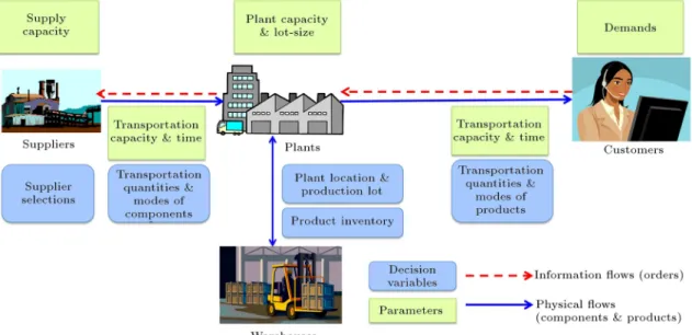
This study considers the electronics industry as the subject to investigate a three-stage multiple-product production-transportation network design that incor-porates suppliers, plants, and customers. Upstream suppliers are component or material vendors represent-ing dierent supplier locations, production capabilities, and ordering costs. Midstream plants are primarily responsible for product manufacturing. Because plant manufacturing capabilities are limited, plant selection is required to ensure sucient production and satisfy customer demand. Downstream represents demand where customers present dierent product demands at dierent times. After incorporating the transportation model, the nal model structure is shown in Figure 1. Plants are the core of the production trans-portation network. The objective of this study is to determine the optimal production batches of a product for each period, component's ordering quantity from each supplier, transported product quantity, product inventory, and transportation quantity corresponding to each transportation mode.

Plants must order components from suppliers based on product requirements. However, suppliers have an upper limit to their supply capability for each period. Suppliers are selected by considering the upper limit of transportation quantity, ordering costs,

component carrying costs, and carbon emissions for various transportation combinations.

This study only considers existing plants for plant selection. Electronic product production frequently requires multiplied amounts of xed production batch size because of production technology or equipment reasons. Thus, in a limited production situation, deci-sion selection involves whether plants should engage in production and when to setup and begin production to fulll the requirements. Because plants are in batch production, unsold products in each period are converted to inventory and sold in the following period. Consumer electronic products are usually manu-factured using core components and the general com-ponents, which can be easily substituted or are similar. This study uses the Bill Of Materials (BOMs) con-cept to describe product and component relationships. Because customer demands change in each period, so does the quantity ordered by each plant from suppliers. Thus, this study assumes that plants order components from suppliers in a lot-for-lot policy; consequently, component inventory or shortages are not considered.

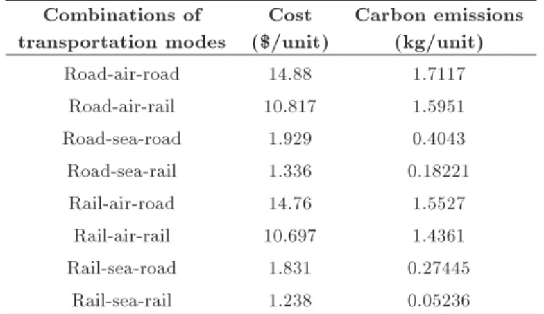
Regarding the transportation dimension, freight forwarders typically assist in the planning of trans-portation mode selection and the delivery of transport components and products. Sea and air transportation are the primary international transportation modes; road and rail are the main land transportation modes. Transportation departure points and endpoints are suppliers to plants or plants to customers. The entire transportation process (e.g., road, rail, air, or sea) can have dierent types of sequences to form compounded transportation modes. For example, a supplier in Fukushima, Japan, uses road (or rail) to ship parts to the Fukushima airport or harbor. The parts are

Table 2. Combinations of transportation modes between Fukushima and Wuhan. Combinations of

transportation modes

Cost ($/unit)

Carbon emissions (kg/unit)

Road-air-road 14.88 1.7117

Road-air-rail 10.817 1.5951

Road-sea-road 1.929 0.4043

Road-sea-rail 1.336 0.18221

Rail-air-road 14.76 1.5527

Rail-air-rail 10.697 1.4361

Rail-sea-road 1.831 0.27445

Rail-sea-rail 1.238 0.05236

then shipped by plane or ship to the Wuhan airport or harbor in China and then transported by road (or rail) to a Wuhan plant for manufacturing into the nal product.

When selecting compound transportation modes, transportation costs and carrying costs are primary considerations. Long transportation distances raise the transportation costs paid by corporations. Each type of transportation combination has its own transportation quantity upper limit. The eight possible transportation combinations, which are applied in this study, cover a range of transportation times, costs, and carbon emis-sions. Example parameters for the transportation com-binations from Fukushima (Japan) to Wuhan (China) are presented in Table 2. Generally, transportation that requires a long time (e.g., maritime shipping) has reduced unit transportation cost and unit carbon emission. These eight transportation combinations will be incorporated in the analyses in Section 4, which entail calculating and converting the transportation distances to obtain the transportation times. Each combination corresponds to the transportation time, cost, and carbon emission parameters of one specic group. The combination formation reduces the symbol complexity of the variables as described in the following sections.

3. Mathematical model and approach 3.1. Symbol denitions

Given that supply chain network, G = (N; A), is composed of numerous nodes and arcs, N represents the nodes in the network: Nodes are divided into suppliers S, plants F , and customers C; thus, N = S [ F [ C. The connection between two nodes is called an arc, and represents one shipping lane candidate for product ow. Each shipping lane consists of multiple transportation combinations. Let '(i; j) be the transportation combinations from node i to node j. For example, '(i; j) = 1 indicates that i to

j uses transportation combination 1 to transportation cargo and = f'(i; j) : (i; j) 2 Ag. If the original G(N; A) from the shipping line perspective is con-verted to the transportation combination perspective, then the supply chain network can be represented by G(N; ). Detailed parameter and variable denitions are provided in the following:

Notations: Indices:

t The index of time periods, and t = 0; 1; 2; 3; :::; T0

r The index of components, and r = 1; 2; 3; :::; R0

p The index of products, and p = 1; 2; 3; :::; P0

Sets:

The set of transportation combinations S The set of suppliers

F The set of facilities C The set of customers R The set of components P The set of products T The set of time periods Parameters:

fct

i The occurring cost when supplier i is

selected at time period t fct

j Setup cost of manufacturing products

at plant j at time period t pct

jp Unit manufacturing cost of product p

at plant j at time period t tct

'(i;j)r Unit transporting cost of component

r from supplier i to plant j using transportation combination '(i; j) at time period t

tct

'(j;k)p Unit transporting cost of product

p from plant j to customer k using transportation combination '(j; k) at time period t

hct

jp Unit holding cost of product p at plant

j at time period t

brp Amount of component r required by

one unit of product p dt

kp Amount of product p required by

customer k at time period t ust

i Supply capacity of supplier i at time

period t uft

j Production capacity of plant j at time

period t usft

'(i;j) Transportation capacity of

transportation combination '(i; j) from supply i to plant j at time period t

ufct

'(j;k) Transportation capacity of

transportation combination '(j; k) from plant j to customer k at time period t

qjp Batch size of product p at plant j

t'(i;j) Transporting time from supplier

i to plant j using transportation combination '(i; j)

t'(j;k) Transporting time from plant j to

customer k using transportation combination '(j; k)

gjp Required production capacity to make

one unit of product p at plant j r Required transportation capacity to

deliver one unit of component r p Required transportation capacity to

deliver one unit of product p

hr Unit holding cost of component r per

period during transportation hp Unit holding cost of product p per

period during transportation et

jp CO2 emissions of manufacturing one

unit of product p at plant j at time period t

et

'(i;j)r CO2emissions of transporting one unit

of component r from supplier i to plant j using transportation combination '(i; j) at time period t

et

'(j;k)p CO2emissions of transporting one unit

of product p from plant j to customer k using transportation combination '(j; k) at time period t

Decision variables: Xt

jp Batches of product p manufactured at

plant j at time period t Xt;t+t'(i;j)

'(i;j)r Transportation quantities of

component r using transportation combination '(i; j) from supplier i at time period t to plant j at time period t + t'(i;j)

Xt;t+t'(j;k)

'(j;k)r Transportation quantities of product

p using transportation combination '(j; k) from plant j at time period t to customer k at time period t + t'(j;k)

Yt

i = 1; If supplier i takes orders at time period

t; Yt

i = 0, otherwise

Yt

j = 1; If plant j operates at time period t;

Yt

j = 0, otherwise

Dependent variables: It

jp Inventory of product p kept at plant j

at time period t 3.2. Mathematical model Objective function 1:

Minimize cost X i2S X t2T fct iYit+

X

j2F

X

t2T

fct jYjt

+X j2F X p2P X t2T pct

jpqjpXjpt

+ X

'(i;j)2

X

r2R

X

t2T :t+t'(i;j)T0

tct

'(i;j)rX'(i;j)rt;t+t'(i;j)

+ X

'(j;k)2

X

p2P

X

t2T :t+t_'(j;k)T0

tct

'(j;k)pXjkpt;t+t'(j;k)

+ X

'(i;j)2

X

r2R

X

t2T :t+t'(i;j)T0

hrt'(i;j)X_'(i;j)rt;t+t'(i;j)

+ X

'(j;k)2

X

p2P

X

t2T :t+t_'(j;k)T0

hpt'(j;k)X'(j;k)pt;t+t'(j;k)

+X j2F X p2P X t2T hct jpIjpt :

(1) Eq. (1) consists of ordering cost charged by sup-pliers, setup cost at plants, production cost at plants, transportation cost of components and products, hold-ing cost while transporthold-ing components and products, and holding cost at plants.

Objective function 2:

Minimize CO2emissions:

X

j2F

X

p2P

X

t2T

et

jpqjpXjpt

+ X

'(i;j)2

X

r2R

X

t2T :t+t'(i;j)T0

et

'(i;j)rX'(i;j)rt;t+t'(i;j)

+ X

'(j;k)2

X

p2P

X

t2T :t+t'(j;k)T0

et

'(j;k)pX'(j;k)pt;t+t'(j;k):

(2) Eq. (2) represents CO2 emissions incurred by

produc-tion at plants, transportaproduc-tion from suppliers to plants, and transportation from plants to customers.

Subject to: X

j2'(i;j)

Xt;t+t'(i;j)

'(i;j)r ustiYit; 8i 2 S; 8r 2 R;

for ft : t + t'(i;j) T0g; (3)

( X

i2'(i;j):t t'(i;j)0

Xt t'(i;j);t

'(i;j)r )=brp= qjpXjpt ;

8j 2 F; 8r 2 R; p 2 P; 8t = T; (4)

I0

jp= 0; 8j 2 F; 8p 2 P; (5)

It 1

jp + qjpXjpt

X

k2'(j;k):t+t'(j;k)T0

Xt;t+t'(j;k)

'(j;k)p =Ijpt ;

8j 2 F; 8p 2 P; 8t = f1; 2; 3; :::; T0_{g; (6)}

X

p2P

gjpqjpXjpt ufjtYjt; 8j 2 F; 8t 2 T; (7)

X

j2'(j;k):t t'(j;k)0

Xt t'(j;k);t

'(j;k)p = dtkp;

8k 2 C; 8p 2 P; 8t 2 T; (8) where dt

kp= 0, if t < min_i2S;j2Fft'(i;j)+ t'(j;k)g.

X

r2R

rX_'(i;j)rt;t+t'(i;j) usf'(i;j)t ;

8'(i; j) 2 : t + t'(i;j) T0; 8t 2 T; (9)

X

p2P

pX_'(j;k)pt;t+t'(j;k) ufct'(j;k);

8'(j; k) 2 : t + t'(j;k) T0; 8t 2 T; (10)

Xt

jp2 Integer; 8j 2 F; 8p 2 P; 8t 2 T; (11)

Xt;t+t'(i;j)

'(i;j)r 0;8'(i; j) 2 : i 2 S; j 2 F; 8r 2 R;

8t 2 T : t + t'(i;j) T0; (12)

Xt;t+t'(j;k)

'(j;k)p 0;

8'(j; k) 2 : j 2 F; k 2 C; 8p 2 P;

8t 2 T : t + t'(j;k) T0; (13)

It

jp 0; 8j 2 F; 8p 2 P; 8t 2 T; (14)

Yt

i 2 f0; 1g ; 8i 2 S; 8t 2 T; (15)

Yt

j 2 f0; 1g ; 8j 2 F; 8t 2 T: (16)

Eq. (3) represents the quantities of transporting com-ponents to plants being less than or equal to the quantities provided by each supplier at each time period. Eq. (4) represents the number of components ordered from suppliers being equal to the number of products manufactured by each plant at each time period. Eq. (5) represents the inventory at plant j being zero at time period 0. Eq. (6) represents ow conservation of each product at each plant at each time period. Eq. (7) represents production capacity at each plant at each time period. Eq. (8) represents the quantities transported to each customer being equal to the demand of each customer at each time period. Since this research assumes that there is no backorder for each customer, the initial demands of each customer are set to 0. Eq. (9) represents the quantities of components transported from suppliers to plants being less than or equal to the capacities of each transporta-tion mode between suppliers and plants at each time period. Eq. (10) represents the quantities of products transported from plants to customers being less than or equal to the capacities of each transportation mode between plants and customers at each time period. Eq. (11) represents the batch size of each product at each plant at each time period, and must be an integer. Eqs. (12) and (13) represent transporting quantities from suppliers to plants and from plants to customers, and the values are non-negative. Eq. (14) represents the amount of inventory, and the value is non-negative. Eqs. (15) and (16) represent the operating status of each supplier and each plant, and the values are binary variables.

3.3. Normalized normal constraint method The solution to multiple-objective decision problems require determining the optimal solution set, not sim-ply a single optimal solution. The Normalized Normal Constraint (NNC) method is a highly eective method of multiple-objective decision optimization that can be used to produce evenly distributed Pareto solutions. This study applies evenly distributed Pareto-optimal fronts to provide managers with improved decisions. The NNC method proposed by Messac et al. [28] is used to calculate a multiple-objective model. This method does not require the calculation of the ini-tial weight of each objective to produce an evenly distributed Pareto-optimal front. Figure 2 illustrates the multiple-objective Pareto-optimal front and utopia line. When using the optimized solutions method of the secularization techniques, both local and global solutions are typically produced, thereby forming non-convex Pareto and discontinuous Pareto solutions [29]. However, the NNC calculation method also produces local and global solutions and exhibits non-convex and discontinuous Pareto solutions [28,30]. Therefore, this study adopts the Pareto lter algorithm proposed by Messac et al. [28] to lter non-optimal solutions on the Pareto curve and obtain the optimal global Pareto solutions. Because of space, constraints please references Messac et al. [28] and Martinez et al. [31] for detailed discussions on Pareto solution procedures and Pareto lters.

The NNC method consists of seven steps [28]:

- Step 1: Two anchor points, 1 _{= (}

11; 12) and

2 _{= (}

21; 22), are calculated (see Figure 2). In

Figure 2, Objective 1 refers to total cost whereas Objective 2 refers to CO2 emissions. 11 is the

minimal total cost of the problem (P1) with the objective function in Eq. (1) subject to Eqs. (3) to

Figure 2. Utopia line and Pareto eciency frontier curve.

(16); 12 is the corresponding CO2 emissions

calcu-lated by the same solution. 22 is the minimal CO2

emissions of the problem (P2) with the objective function in Eq. (2) subject to Eqs. (3) to (16); 21is

the corresponding total cost calculated by the same solution.

- Step 2: A normalization based on (1_; 2_{) is}

performed because of the dierent units (NT dollars and kg) of Objectives 1 and 2. After running the normalization, is calculated by using Eq. (17):

=

1(x) 1(x1)

1(x2) 1(x1);

2(x) 2(x2)

2(x1) 2(x2)

; (17) where the Euclidean distance between 1 _{= (0; 1)}

and the origin = (0, 0) is 1; similarly, the Euclidean distance between 2 _{= (1; 0) and the origin = (0,}

0) is 1.

- Step 3: The utopia line vector (N = 2 1_),

which is the direction from 1 _to 2_{, is calculated.} - Step 4: A normalized increment m is calculated. In

this study, m is 30.

- Step 5: Utopia line points, Xj, using Eq. (18) are

generated: Xj =

1

m 1 1; (1 1

m 1) 2

;

for j= 1; 2; ;m 1: (18)

- Step 6: Each Pareto-point problem, which is the problem (P2), is solved with the objective function in Eq. (2) subject to Eqs. (3) to (16) and the corresponding Eq. (19):

N(₂ Xj)T 0; (19)

₂ is a point within the feasible region of P2, and the optimal solution of P2 is the point of

2. - Step 7: The real value () of each Pareto point,

2, is calculated by calculating the inverse of the

normalization in Eq. (20):

=[1(1(x2) 1(x1)) + 1(x1); 2(2(x1)

2(x2)) + 2(x2)]T: (20)

4. Case study and numerical analysis

This section presents how the study substitutes data into the mathematical programming model to examine the network design issues in green supply chains. Pa-rameter value changes are used to observe the response status of the entire supply chain. The solution process uses ILOG CPLEX 12.4 to conduct calculations (using an Intel Core i5-2400 CPU with a 3.10 GHz central processor, 8 GB of memory, and the Windows 7 Professional Edition operating system).

4.1. Case study

This study extends the case company background used by Wang et al. [18] and obtains the supplier sources, current plant locations, and customer locations by reviewing references (Figure 3). Assuming that the main sources for components are South Korea, Japan, and Thailand and the assembly plants are distributed in several cities in Taiwan and China, the assembly plants would provide products to local customers.

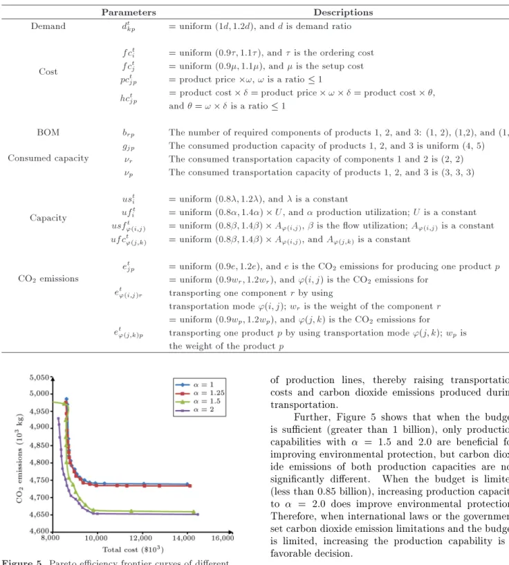
The case supply chain network comprises three suppliers, four plants, and four customers. To simplify analysis, three products and 12 planning horizon pe-riods are used in this study. Relevant data, such as the product carbon emission coecients produced by the plants, are obtained from sustainable development reports on products similar to the case company prod-ucts. The carbon emission coecients produced by the transportation tools are collected using SimaPro 7.3. software. Transportation distances are measured ac-cording to Google Maps. Detailed numerical denitions for the parameters are presented in Table 3. These data are used to obtain the optimal component order quan-tity, production batch, product delivery quanquan-tity, and plant location for various transportation combinations and periods. The data in this example are used to set the demand for the rst two periods at zero to ensure that supply shortages do not occur. A set amount of initial product inventory can also be assumed to satisfy initial demand.

Because the ILOG CPLEX 12.4 involves using a branch-and-bound search method in the internal settings during the integer solution process, excessive factors and data in the integer-programming model can overload the memory, resulting in lacking solutions. Therefore, a 1% tolerance deviation is set when search-ing for the optimal integer solutions. Cordeau et al. [32] asserted that, in practice, a deviation exceeding 1%

Figure 3. Supply chain network of the case company.

Figure 4. Pareto eciency frontier curve.

frequently occurred in company data sources (e.g., esti-mations of costs, demands, and production capability); thus, a 1% variation is within the allowable range.

The optimal total cost and carbon emission combinations in the Pareto-optimal front curve are shown in Figure 4. The two terminal points are NT$862,269,800 and 4,985,400 kg, and $1,398,400,000 and 4,738,968 kg, respectively. The gure shows the balance between total cost and carbon dioxide emis-sions. From a marginal utility perspective (e.g., using the farthest left point as the benchmark), the supply chain network design combination corresponding to NT$941,860,000 and 4,750,100 kg is recommended to corporations. Increasingly stringent restrictions on car-bon dioxide generate rapidly increasing cost; however, these eects, which are produced by various factors, are dicult to observe. Thus, in the next section, sensitivity analysis of several main factors is shown to understand how alterations in a variety of factors inuence the supply chain network, and this research examines corporate-response decisions.

4.2. Sensitivity analysis

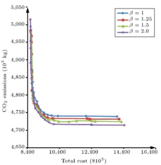
4.2.1. Change in plant production capability

To understand how changes in plant production ca-pability aect decisions, this study adjusts the upper production limit according to three values ( = 1:25, 1.5, and 2.0) to obtain three groups of Pareto-optimal fronts. These three Pareto-optimal fronts are compared with those obtained using the original = 1. Figure 5 shows that when production capability increases, costs decrease, resulting in a shift of the entire curve toward the initial point. This indicates that, at the same cost, increased production capacities generate fewer carbon dioxide emissions. In a xed carbon dioxide emission situation, high production capacity reduces the total cost because increasing plant production capability reduces the required number of transports, thereby reducing transportation costs and concurrent carbon dioxide emissions. Fewer transports reduce the overall

Table 3. Parameter data set.

Parameters Descriptions

Demand dt

kp = uniform (1d; 1:2d), and d is demand ratio

Cost

fct

i = uniform (0:9; 1:1), and is the ordering cost

fct

j = uniform (0:9; 1:1), and is the setup cost

pct

jp = product price !, ! is a ratio 1

hct

jp = product cost = product price ! = product cost ;_{and = ! is a ratio 1}

BOM brp The number of required components of products 1, 2, and 3: (1, 2), (1,2), and (1,2)

Consumed capacity

gjp The consumed production capacity of products 1, 2, and 3 is uniform (4, 5)

r The consumed transportation capacity of components 1 and 2 is (2, 2)

p The consumed transportation capacity of products 1, 2, and 3 is (3, 3, 3)

Capacity

ust

i = uniform (0:8; 1:2), and is a constant

uft

i = uniform (0:8; 1:4) U, and production utilization; U is a constant

usft

'(i;j) = uniform (0:8; 1:4) A'(i;j), is the ow utilization; A'(i;j)is a constant

ufct

'(j;k) = uniform (0:8; 1:4) A'(i;j), and A'(j;k)is a constant

CO2 emissions

et

jp = uniform (0:9e; 1:2e), and e is the CO2emissions for producing one product p

et '(i;j)r

= uniform (0:9wr; 1:2wr), and '(i; j) is the CO2 emissions for

transporting one component r by using

transportation mode '(i; j); wris the weight of the component r

et '(j;k)p

= uniform (0:9wp; 1:2wp), and '(j; k) is the CO2 emissions for

transporting one product p by using transportation mode '(j; k); wp is

the weight of the product p

Figure 5. Pareto eciency frontier curves of dierent production capacity ratios.

transportation time; consequently, increased produc-tion yields a reducproduc-tion in carbon dioxide emissions and thereby causes less harm to the environment. This phenomenon is similar to that described by Wang et al. [18]. Reduction in plant production capacity signi-es that customer product demand must be supported by production from other plants or additional setup

of production lines, thereby raising transportation costs and carbon dioxide emissions produced during transportation.

Further, Figure 5 shows that when the budget is sucient (greater than 1 billion), only production capabilities with = 1:5 and 2.0 are benecial for improving environmental protection, but carbon diox-ide emissions of both production capacities are not signicantly dierent. When the budget is limited (less than 0.85 billion), increasing production capacity to = 2:0 does improve environmental protection. Therefore, when international laws or the government set carbon dioxide emission limitations and the budget is limited, increasing the production capability is a favorable decision.

4.2.2. Change in the upper limit of transportation quantity

Dierent transportation tools have dierent portation quantity limits. To understand how trans-portation quantity changes inuence decisions, this study adjusts the production capability rate and sets three values as the upper limit of the transportation quantity rate (i.e., = 1:25, 1.5, and 2.0) to obtain three groups of Pareto-optimal fronts. These three

Figure 6. Pareto eciency frontier curves of dierent upper bound ratios of transportation capacities.

Pareto-optimal fronts are compared with that obtained using the original = 1. Figure 6 shows that, except for the = 2:0 curve, the other three curves are the same in the high carbon emission stage. Furthermore, both carbon emissions and total cost decrease when transportation quantity increases. The researchers learnt that when transportation quantity was limited, the limits of corporate component or product trans-portation raised because variations in transtrans-portation costs resulted in high carbon dioxide emissions. Thus, raising the transportation improves the exibility of the entire supply chain.

Figure 6 shows that when the budget is sucient (greater than 1 billion NT dollars), increasing trans-portation quantity limits will be slightly benecial for improving environmental protection. When the budget is limited (less than 0.9 billion NT dollars), increasing transportation quantity limits is not benecial for improving environmental protection. Therefore, trans-portation quantity limits is not a sensitive parameter. 4.2.3. Changes in production batch size

To understand the inuence of the size of plant pro-duction batches, this study adjusts propro-duction batch size ratio to compare = 1:5 and = 2:0 with the original = 1. Figure 7 shows that when the carbon dioxide limit is 490,000 kg, plants with the small production batch size reduce the total cost. Figure 7 also shows that when the production batch size increases, total cost increases. However, total costs are not signicantly dierent for the production batch sizes = 1:5 and = 2:0. The possible reason may be that when customer demands are known and xed, plants must produce more products due to large production batch sizes. Therefore, when the

Figure 7. Pareto eciency frontier curves of dierent production batch size ratios.

production batch sizes increase, ordering component, transportation, carrying, and total costs also increase. In practice, companies prefer the large production batch sizes to small ones, because large production batch sizes can shorten the setup time of machines and be easily scheduled in the production lines. Further, surplus products can be stored for the next-period cus-tomer demands. However, the large production batch sizes will increase the transportation and carrying costs and carbon dioxide emissions. There is a trade-o between production preference (large production batch sizes) and total cost (small production batch sizes). Therefore, companies should determine appropriate production batch sizes based on their product char-acteristics, cost, and environmental factors. This topic merits further research.

5. Conclusion

This study proposed a green supply chain network model that involved calculating multi-phase, multiple-objective integer programming models. The supply chain network model also incorporated carbon emis-sions, including those produced during the transporta-tion process. The model used the selectransporta-tion of trans-portation type to reduce carbon emissions during the transportation process. This model can be used by corporations when considering localized environmental inuences or globalized supply chain network designs.

Section 3 introduced the mathematical model developed in this study. Section 4 provided examples, sensitivity analysis results, and a discussion of manage-ment implications. Figure 5 indicated that production capability increases were benecial for improving envi-ronmental conditions. However, additional costs were required to increase production capability. When car-bon dioxide emissions were high, increasing production capability only slightly reduced the total cost. The

Pareto curve trends can serve as a reference for decision makers when determining the benets for companies generated by increasing production capability.

Lowering the upper transportation quantity limit required plants to order the necessary product-assembly components from additional suppliers (in-creasing the number of suppliers), thereby raising the ordering costs. Similarly, the number of times the plant set up production also increased, generating setup production costs. Ordering components and transport-ing manufacturtransport-ing products became complex, caustransport-ing uctuations in transportation costs and increasing total costs. Figure 6 can be used as a reference for decision makers when determining whether increasing the upper transportation quantity limit would benet the company.

Total costs rose when the production batch sizes increased, because this production process required the ordering of additional components. Thus, each time components were ordered represented an increase in transportation and carrying costs. When production managers plan multi-phase production activities, the manufactured multi-phase products from each pro-duction batch are stored in inventory to ensure that customer demand in the following period is satised. A large production batch size from the plant signies that numerous products are available for storing into inventory and fullling multi-period customer demand. Reducing the number of production setups reduces setup costs. However, the transportation and carrying costs produced by the components raised costs. There is a trade-o between production batch size and total cost. Therefore, determining appropriate production batch sizes remains a challenging research topic.

Although this study used the electronics industry as the core, numerous factors were excluded from con-sideration when exploring overall supply chain planning in the production and delivery model. These factors can be considered in future studies:

1. This study considered transportation time, but not the product shortage costs resulting from delayed deliveries subsequent to insucient production ca-pability or transportation delays [3]. Therefore, future studies should discuss the inuence of these factors on supply chain production and delivery;

2. This study also did not consider uctuating cus-tomer product demands [33,34]. Thus, product demand uncertainty should be added to the model to conform to actual situations.

Acknowledgement

This research was partially supported by Chang Gung Memorial Hospital under Grant BMRPE93.

References

1. Trucost, \Carbon emissions - measuring the risks" (2009).

2. Beamon, B.M. \Supply chain design and analysis: Models and methods", International Journal of Pro-duction Economics, 55(3), pp. 281-294 (1998). 3. Melnyk, S.A., Narasimhan, R. and DeCampos, H.A.

\Supply chain design: Issues, challenges, frameworks and solutions", International Journal of Production Research, 52(7), pp. 1887-1896 (2014).

4. Aliev, R.A., Fazlollahi, B., Guirimov, B.G. and Aliev, R.R. \Fuzzy-genetic approach to aggregate production-distribution planning in supply chain man-agement", Information Sciences, 177(20), pp. 4241-4255 (2007).

5. Badri, H., Ghomi, S.M.T.F. and Hejazi, T.H. \A two-stage stochastic programming model for value-based supply chain network design", Scientia Iranica Transaction E, Industrial Engineering, 23(1), pp. 348-360 (2016).

6. Mahmoodirad, A. and Sanei, M. \Solving a multi-stage multi-product solid supply chain network design problem by meta-heuristics", Scientia Iranica, Trans-action E, Industrial Engineering, 23(3), pp. 1428-1440 (2016).

7. Melo, M.T., Nickel, S. and Saldanha-da-Gama, F. \Facility location and supply chain management - A review", European Journal of Operational Research, 196(2), pp. 401-412 (2009).

8. Rizk, N., Martel, A. and D'Amours, S. \Multi-item dynamic production-distribution planning in process industries with divergent nishing stages", Computers & Operations Research, 33(12), pp. 3600-3623 (2006). 9. Nishi, T., Konishi, M. and Ago, M. \A distributed decision making system for integrated optimization of production scheduling and distribution for aluminum production line", Computers & Chemical Engineering, 31(10), pp. 1205-1221 (2007).

10. Kanyalkar, A.P. and Adil, G.K. \An integrated aggre-gate and detailed planning in a multi-site production environment using linear programming", International Journal of Production Research, 43(20), pp. 4431-4454 (2005).

11. Hugo, A. and Pistikopoulos, E.N. \Environmentally conscious long-range planning and design of sup-ply chain networks", Journal of Cleaner Production, 13(15), pp. 1471-1491 (2005).

12. Das, K. and Sengupta, S. \A hierarchical process industry production-distribution planning model", In-ternational Journal of Production Economics, 117(2), pp. 402-419 (2009).

13. Sadjady, H. and Davoudpour, H. \Two-echelon, multi-commodity supply chain network design with mode selection, lead-times and inventory costs", Computers & Operations Research, 39(7), pp. 1345-1354 (2012).

14. Yang, C.C. \A DEA-based approach for evaluating the opportunity cost of environmental regulations", Asia-Pacic Journal of Operational Research, 30(2), p. 1250049 (1-17) (2013).

15. Forouzanfar, F., Tavakkoli-Moghaddam, R., Bashiri, M. and Baboli, A. \A new bi-objective model for a closed-loop supply chain problem with inventory and transportation times", Scientia Iranica, Transac-tion E, Industrial Engineering, 23(3), pp. 1441-1458 (2016).

16. Ramezani, M., Kimiagari, A.M. and Karimi, B. \Inter-relating physical and nancial ows in a bi-objective closed-loop supply chain network problem with un-certainty", Scientia Iranica, Transaction E, Industrial Engineering, 22(3), pp. 1278-1293 (2015).

17. Cruz, J.M. \Dynamics of supply chain networks with corporate social responsibility through integrated en-vironmental decision-making", European Journal of Operational Research, 184(3), pp. 1005-1031 (2008). 18. Wang, F., Lai, X.F. and Shi, N. \A multi-objective

optimization for green supply chain network design", Decision Support Systems, 51(2), pp. 262-269 (2011). 19. Ferretti, I., Zanoni, S., Zavanella, L. and Diana, A.

\Greening the aluminium supply chain", International Journal of Production Economics, 108(1-2), pp. 236-245 (2007).

20. Cholette, S. and Venkat, K. \The energy and carbon intensity of wine distribution: A study of logistical options for delivering wine to consumers", Journal of Cleaner Production, 17(16), pp. 1401-1413 (2009). 21. Paksoy, T. \Optimizing a supply chain network with

emission trading factor", Scientic Research and Es-says, 5(17), pp. 2535-2546 (2010).

22. Chiu, C.Y., Lin, Y. and Yang, M.F. \Applying fuzzy multiobjective integrated logistics model to green sup-ply chain problems", Journal of Applied Mathematics, Article ID 767095, pp. 1-12 (2014).

23. Jamshidi, R., Fatemi Ghomi, S.M.T. and Karimi, B. \Multi-objective green supply chain optimization with a new hybrid memetic algorithm using the Taguchi method", Scientia Iranica, Transaction E, Industrial Engineering, 19(6), pp. 1876-1886 (2012).

24. Al-e-hashem, S.M.J.M., Baboli, A. and Sazvar, Z. \A stochastic aggregate production planning model in a green supply chain: Considering exible lead times, nonlinear purchase and shortage cost functions", Eu-ropean Journal of Operational Research, 230(1), pp. 26-41 (2013).

25. Fahimnia, B., Sarkis, J., Boland, J., Reisi, M. and Goh, M. \Policy insights from a green supply chain opti-misation model", International Journal of Production Research, 53(21), pp. 6522-6533 (2015).

26. Coskun, S., Ozgur, L., Polat, O. and Gungor, A. \A model proposal for green supply chain network design based on consumer segmentation", Journal of Cleaner Production, 110, pp. 149-157 (2016).

27. Entezaminia, A., Heydari, M. and Rahmani, D. \A multi-objective model for multi-product multi-site ag-gregate production planning in a green supply chain: Considering collection and recycling centers", Journal of Manufacturing Systems, 40, pp. 63-75 (2016). 28. Messac, A., Ismail-Yahaya, A. and Mattson, C.A. \The

normalized normal constraint method for generating the Pareto frontier", Structural and Multidisciplinary Optimization, 25(2), pp. 86-98 (2003).

29. Logist, F., Houska, B., Diehl, M. and Impe, J.V. \Fast Pareto set generation for nonlinear optimal control problems with multiple objectives", Structural and Multidisciplinary Optimization, 42(4), pp. 591-603 (2010).

30. Das, I. and Dennis, J.E. \Normal-boundary intersec-tion: A new method for generating the Pareto sur-face in nonlinear multicriteria optimization problems", SIAM Journal on Optimization, 8(3), pp. 631-657 (1998).

31. Martinez, M., Sanchis, J. and Blasco, X. \Global and well-distributed Pareto frontier by modied normal-ized normal constraint methods for bicriterion prob-lems", Structural and Multidisciplinary Optimization, 34(3), pp. 197-209 (2007).

32. Cordeau, J.F., Pasin, F. and Solomon, M.M. \An integrated model for logistics network design", Annals of Operations Research, 144(1), pp. 59-82 (2006). 33. Rangel, D.A., Oliveira, T.K.d. and Leite, M.S.A.

\Sup-ply chain risk classication: Discussion and proposal", International Journal of Production Research, 53(22), pp. 6868-6887 (2015).

34. Wakolbinger, T. and Cruz, J.M. \Supply chain disrup-tion risk management through strategic informadisrup-tion acquisition and sharing and risk-sharing contracts", International Journal of Production Research, 49(13), pp. 4063-4084 (2011).

35. Pyke, D.F. and Cohen, M.A. \Performance character-istics of stochastic integrated production-distribution systems", European Journal of Operational Research, 68(1), pp. 23-48 (1993).

36. Melkote, S. and Daskin, M.S. \Capacitated facility location/network design problems", European Journal of Operational Research, 129(3), pp. 481-495 (2001). 37. Eksioglu, S.D., Romeijn, H.E. and Pardalos, P.M.

\Cross-facility management of production and trans-portation planning problem", Computers & Operations Research, 33(11), pp. 3231-3251 (2006).

38. Farahani, R.Z. and Elahipanah, M. \A genetic algo-rithm to optimize the total cost and service level for just-in-time distribution in a supply chain", Interna-tional Journal of Production Economics, 111(2), pp. 229-243 (2008).

39. Selim, H., Am, C. and Ozkarahan, I. \Collaborative production-distribution planning in supply chain: A fuzzy goal programming approach", Transportation Research Part E-Logistics and Transportation Review, 44(3), pp. 396-419 (2008).

40. Liang, T.-F. \Fuzzy multi-objective production/dist-ribution planning decisions with multi-product and multi-time period in a supply chain", Computers & Industrial Engineering, 55(3), pp. 676-694 (2008). 41. Al-e-hashem, S.M.J.M., Malekly, H. and Aryanezhad,

M.B. \A multi-objective robust optimization model for multi-product multi-site aggregate production plan-ning in a supply chain under uncertainty", Interna-tional Journal of Production Economics, 134(1), pp. 28-42 (2011).

42. Rezaei, J. and Davoodi, M. \Multi-objective models for lot-sizing with supplier selection", International Journal of Production Economics, 130(1), pp. 77-86 (2011).

43. Liu, S.S. and Papageorgiou, L.G. \Multiobjective opti-misation of production, distribution and capacity plan-ning of global supply chains in the process industry", Omega-International Journal of Management Science, 41(2), pp. 369-382 (2013).

Biographies

Dah-Chuan Gong is a Professor in the Department of Industrial and Business Management at Chang Gung University, Taiwan, ROC. He obtained a PhD degree from the School of Industrial and Systems Engineering, Georgia Institute of Technology, USA. His research area focuses on global logistics management, sustain-able supply chain management, production system design, and operations research applications.

Ping-Shun Chen is an Associate Professor in the Department of Industrial and Systems Engineering at Chung Yuan Christian University, Taiwan, ROC. He obtained a PhD degree from the Department of Industrial and Systems Engineering, Texas A&M Uni-versity, USA. His research area focuses on network pro-gramming or applications, supply chain management, healthcare applications, and system simulation. Tzu-Yang Lu is a master student in the Department of Industrial and Systems Engineering at Chung Yuan Christian University, Taiwan, ROC. His research area focuses on analyses of the supply chain network design.