Vol. 2, No. 2, pp 114-125 Summer 2008
A Non-parametric Control Chart for Controlling Variability Based on
Squared Rank Test
Nandini Das
SQC-OR Unit, Indian Statistical Institute, 203 B T Road, Kolkata-700108, India [email protected]
ABSTRACT
Control charts are used to identify the presence of assignable cause of variation in the process. Non-parametric control chart is an emerging area of recent development in the theory of SPC. Its main advantage is that it does not require any knowledge about the underlying distribution of the variable. In this paper a non-parametric control chart for controlling variability has been developed. Its in control state performances have been computed for different distributions and compared with existing Shewhart S chart. Its efficiency to detect shift in variability has been evaluated.
Keywords: Non-parametric control chart, Variability, ARL, Power of a test, OC curve. 1. INTRODUCTION
One of the primary goals of SPC or statistical process control is to distinguish between two sources of variation, those which cannot be economically identified and corrected (chance cause) and those which can be (assignable cause). When a process operates only under chance causes, it is said to be in a state of statistical control. Control charts are used to detect whether a process stays in a state of statistical control. That is, they assess whether the distribution of the quality characteristic (Xt), or
its parameter such as mean or variability remain at their specified levels.
In the context of process control, it is assumed that the pattern of chance causes follows a stable probability distribution. The control limits of traditional Shewhart type control chart is derived based on the assumption that the distribution of this pattern is normal. The statistical properties of commonly employed control charts are exact only if the assumption is satisfied; however, the underlying process is not normal in many practical situations, and as a result the statistical properties of standard charts can be highly affected in such situations. On this point see Shewhart (1939), Ferrell (1953), Tukey (1960), Langenberg and Igelewicz (1986), Jacobs (1990), Alloway and Raghavachari (1991), Yourstone and Zimmer (1992), Woodall and Montgomery (1999), Woodall (2000).
Distribution-free or nonparametric control charts are parallel alternatives if one is concerned about non-normality and contamination. It should be noted that this term nonparametric is not intended to imply that there are no parameters involved. Some non-parametric procedures actually outperformed their parametric counterparts remarkably even when the underlying distribution is in fact normal, the (asymptotic relative) efficiency of some non-parametric methods (e.g ,the Wilcoxon signed-rank test ) relative to the corresponding (optimal ) normal theory methods( the t
test ) is as high as 0.955 . Finally to be fair it is noted that a large part of the developments in the non-parametric methodology have taken place in the classical confines of statistical estimation and hypothesis testing and not enough effort has been made to understand the problems of statistical process control.
The main advantage of non-parametric control charts is the flexibility derived from not needing to assume any parametric probability distribution for the underlying process; at least as far as establishing and implementing the charts are concerned. Obviously, this is very beneficial in the field of process control, particularly in start-up situations where not much data is available to use a parametric (e.g normal theory) procedure. Also, the nonparametric charts are likely to share the robustness properties of non-parametric tests at confidence intervals and are ,therefore, far more likely to be less impacted by outliers.
It should be noted that non-parametric methods can be somewhat less efficient than their parametric counterparts, provided ofcourse that one has a complete knowledge of the underlying stochastic process for which the particular parametric method is specifically designed; however, the reality is that such information is seldom, if ever, available to the quality practitioners. Moreover, in today’s computer based process monitoring and control, “less efficiency” can often be compensated for by more observations. Another perceived disadvantage of non-parametric charts is that for small sample sizes one needs special tables. Again, this should not be a problem given the ubiquitous presence of computers today.
There exist a number of nonparametric control charts for controlling location parameter viz., mean and median which are described in the next section. Since few works are reported in the literature on the non-parametric control chart for controlling variability or scale parameter we have proposed a non parametric control chart for controlling variability when location parameter is under control. The performance of the proposed methods will be assessed for both in-control state and out-of-control state under different underlying distributions.
2. LITERATURE SURVEY
A survey of recently available literature reveals the development of a substantial number of non-parametric control charts where no underlying distribution is assumed on the process output. Woodall and Montgomery (1999) foresaw an increasing role for non-parametric methods in control charting application. Chakraborti et al. (2001) gave an overview and discussed the advantages of several non-parametric control charts over their normal theory counterparts. Bakir (2001) complied and classified several non-parametric control charts according to the driving non-parametric idea behind each one of them.
Bakir and Reynolds (1979) used within group sign ranks to develop CUSUM charts. Alloway and Raghavachari, (1991) considered a Shewhart type chart for the point of symmetry
θ
of a continuous, symmetric population based on a distribution free confidence interval forθ
, calculated using Hodges-Lehmann estimator. Amin, et. al., (1995) present nonparametric control charts for process median (or the mean) based on sign test statistic. Altukife, (2003) considered two more control charts based on the “grand median” and “sum of ranks”. However these charts can not be considered distribution free since the chart constants are derived for each of the four parametric distributions he considered.Apart from these, Park and Reynolds, (1987) developed nonparametric Shewhart type procedures for monitoring the location parameter of a continuous process when the in-control value for the
parameter is not specified based on the “linear placement” statistics, introduced by Orban and Wolfe, (1982) for comparing current samples with a standard sample taken when the process is operating properly. Asymptotic approximations to the run length distributions are obtained. Pappanastos and Adams, (1996) modified the Alloway-Raghavachari charts whereas Willeman and Runger, (1996) considered designing control charts using so-called “empirical reference distribution.” Bakir (2006) developed a non-parametric control chart based on sign ranked like statistics when in-control process center is not specified. Qiu and Hawkins (2003) developed a non-parametric multivariate CUSUM control chart. Bhattacharya and Frierson (1981) developed a nonparametric control chart to detect small shifts. Zhou et al. (2007) worked on non-parametric control charts based on change point estimate.
All the control charts mentioned above are used to check whether the process is under control with respect to the location parameter assuming that variability is under control. But to validate the assumption we need to have some control chart for monitoring variability.
When it is necessary to monitor the variance as well as the center of distribution, then a chart for variability will usually be used, such as R, S, or the S2 charts. The R chart is less efficient than the
corresponding S2 chart when the underlying distribution is normal. The S2 chart for monitoring an increase in process variability gives a signal if S2 exceeds the control limit a3= σ2 χ2ά, where χ2α denotes the upper α percentage point of the chi-square distribution with (n-1) degrees of freedom, and σ2 is an estimate of the process variance. It is a common practice to estimate σ from process data, and then to use the appropriate percentage point of the chi-square distribution in setting up the control limits. The probability limits above are only appropriate with normal data, and the ARL for the S2 chart depends heavily on using the correct constants in setting up the control limits. We are
unaware of any published work on the appropriate control limits of control charts for variability when the underlying distributions are non-normal.
The effects of non-normality are more severe in control charts for variability than in the case of carts for location.
The variance of
S
2 is given by,) 2
) 1 ( 1 ( ) 1 (
2 )
( 2 4 2
n n n
S
V + −
−
=
σ
γ
Where, γ2 is the coefficient of kurtosis. Wetherill and Brown (1991) point out that the kurtosis of
the original distribution can have a large effect on the variance of S2, and that effect does not disappear with an increase of sample size.
Though a few nonparametric control charts for location have been reported in the literature, control charts on variability are really scarce. Lehman(1975) adopted nonparametric tests for the equality of two variances as control statistics in nonparametric control charts for variability. Control charts using test statistics for comparing two variances would require obtaining an initial sample(of size
m) when the process is considered to be in-control. Then at each sample time I, a sample of size n is obtained from the process, and the pooled sample of size (m+n) is obtained. The observations in the pooled sample are then ranked from smallest to largest and some statistics based on the ranks of the observation are calculated.
Another approach was given by Bradley (1968) based on Westenberg’s Two-Sample Interquartile Range Test. The test is based on pooling two samples S1andS2, into one sample and then counting the number of observations belonging to the S1 sample that are above third quartile (
Q
3) or below the first quartile (Q1), where Q1andQ
3are based on the pooled sample. It is proposed to adapt the idea of this test to the one sample case as a control procedure. In the control chart applications,1
Q and
Q
3 would need to be specified by process engineers or more likely estimated from process data when the process is in control. Let,⎪ ⎩ ⎪ ⎨ ⎧ < < − = = > < = 3 1 3 1 3 1 1 or 0 or 1 Q X Q if Q X Q X if Q X Q X if U ij ij ij ij ij ij
where
X
ij is the jth observation in the ith. sample. The sign statistic at samplei
is∑
= = n j ij i U U 1 , and the random variable
V
i=
(
U
i+
n
)
/
2
follows a binomial distribution with parameters n and) (X Q3orX Q1 P
p = ij > ij < . A signal is given if
V
i≥
c
, whereV
i is the number of observedij
X
’s that exceedQ
3 plus the number of observedX
ij’s that fall below Q1 in the ith. Sample. Some of the recent works on control chart for monitoring variability are described below.Riaz (2008) developed a Shewhart type control chart namely Vr chart for improved monitoring of
process variability (targeting large shifts) of a quality characteristic of interest Y. The proposed control chart is based on regression type estimator of variance using a single auxiliary variable X. It is assumed that (Y, X) follow a bivariate normal distribution. Its comparison is made with the well-known Shewhart control chart namely S2 chart used for the same purpose. Using power curves as a
performance measure it is observed that Vr chart outperforms the S2 chart for detecting moderate to
large shifts, which is the main target of Shewhart type control charts, in process variability under certain conditions on ρxy . These efficiency conditions on ρxy are also obtained for Vr chart in this
study.
Kao and Ho (2005) worked on optimal transformation coefficients for use in transforming the sample variances for statistical process control (SPC) applications. The optimal exponents for transformation were determined by minimizing the sum of absolute differences between two distinct cumulative probability functions. The normal distribution well approximates the transformed distribution. The operating characteristic (OC) curves were calculated, presented and compared to those of a normal distribution. The analytical results demonstrate that the OC curve of the proposed transformation method is better than that of the log transformation of the sample variance (lns2).
Kiani et al. (2008) developed two new charts based approximately on the normal distribution. The constant values needed to construct the new control limits are dependent on the sample group size (k) and the sample subgroup size (n). Additionally, the unknown standard deviation for the proposed approaches was estimated by a uniformly minimum variance unbiased estimator (UMVUE). This estimator has a variance less than that of the estimator used in the Shewhart and Bonferroni approaches. The proposed approaches in the case of the unknown standard deviation,
give out-of-control average run length slightly less than the Shewhart approach and considerably less than the Bonferroni-adjustment approach.
It is worthwhile to note here the works done by Riaz (2008), Kao and Ho (2005) and Kiani et al. (2008) are not nonparametric control charts.
Das (2008) proposed a nonparametric control chart for monitoring variability based on two sample rank-sum test on dispersion by Ansari and Bradley (1960). Its in control ARL performance is very good but out of control performance with respect to detecting the shift in variability is not up to the mark.
Proposed Nonparametric control chart based on Conover’s squared rank test for variance (Conover , 1980) proposed a test for equality of variances based on the joint squared ranks of squared deviations from the means. Let
X
=
(
X
1,...
X
m)
andY
=
(
Y
1,...
Y
n)
represent two independent samples of size m and n respectively. The squared deviations from the means are(
X
i−
μ
X)
2,(
Y
i−
μ
Y)
2 whereμ
Xandμ
Y are the respective means ofX
andY
.The population means are seldom known but it is reasonable to replace them by their sample estimatesX
m andmY. We do not need to square the deviations to obtain the required rankings because the same order is achieved by ranking the absolute deviations Xi −mX , Yi −mY . These deviations are ranked and the square of the ranks are considered as corresponding scores. The test statistic
T
is the sum of scores of these ranks for one of the samples. For large sample,)
(
))
(
(
T
V
T
E
T
Z
=
−
has a standard normal distribution, whereE
(T
)
andV
(T
)
can be found using∑
+ =
+
= m n
j j s n m m T E 1 ) ( ) ( ) (
and ( 1 ( ) )
) 1 )( ( ) ( 1 2 1 2
∑
∑
+ = + = + − − + += m n
j j n m j j s n m s n m n m mn T
V ,
s
i is the score for the ith orderedobservation in the joint sample. Conover (1980) gives quartiles of
T
for a range of sample sizes in a no tie situation. Programs generating the permutation distribution for arbitrary scores may also be used if exact tail probabilities are required. The detailed theory can be obtained from Conover, (1980) and Sprent (1989).The above mentioned non-parametric test of equality of two variances is considered to set up a control chart for controlling variability. Here we have used the test for each of the two consecutive samples. More elaborately, equality of variances of sample-1 and that of sample-2 is tested and standardized test statistic is to be plotted against the standardized limits (+3 and –3). Then the same hypothesis is tested considering sample-2 and sample-3 and the standardized test statistic is plotted in the same chart and so on.
Steps for control chart:
Step 1: Collect k (at least 20) samples of size n.
Step 2: For each two consecutive samples compute T. In this way k-1 values of T will be computed. Step 3: Find E(T) and Var(T).
Step 4: Calculate Standardized T or Z statistics for each pair of samples. Step 5: Set the control chart parameters as
Upper control limit (UCL) = 3 Central line = 0;
Lower control limit (LCL) = -3
Step 6 : Plot Z values in the control chart. If any point goes beyond the limit it will indicate that the process is out of control with respect to variability.
3. PERFORMANCE OF THE PROPOSED CHART
A popular measure of chart performance is the expected value of the run length (the number of samples or subgroups that need to be collected before the first out of control signal is given by a chart is a random variable called the run length.) distribution called the average run length (ARL). By definition, the run length is a positive integer valued random variable, so the ARL loses much of its attractiveness as a typical summary if the distribution is skewed (as is often the case). It is desirable (often stipulated) that the ARL of a chart be large when the process is in control. Larger the value of the in control ARL, the better the performance of the chart with respect to false alarms. The main task of a control chart is to detect the change in the process as quickly as possible and give an out-of–control signal. Clearly the quicker the detection and the signal, the more efficient the chart is. A second measure as percentage of correct classification to detect different shifts in variance may serve the above purpose. Larger the value of the % correct classification for a particular shift greater the efficiency of the chart to detect the shift. In this paper we have considered % correct classification of the proposed chart as measure of its ability to detect a shift in variability as λσ0 where σ0 is the process standard deviation when the process is under control.
Computer programs written in MATLAB 7.0.1 are used to study the performance of the control charts under different distributions: Normal, Uniform, Laplace, Gamma and Beta using a simulation based on 10000 runs for sample sizes of n=10, 15 and 20.
The density functions of different distributions considered in the study are as follows: Normal distribution: exp(-½(x-μ)2/σ2))/((√(2π)σ)
For this study, we have considered μ = 50 and σ = 5 Gamma distribution: αp exp(-αx)/Γ(p)
For this study, we have considered (α = 1, p=3.5) and (α = 1, p=6) Beta distribution: xm-1(1-x)ν-1/β(m,ν)
For this study, we have considered m = 3, ν=3 Uniform distribution: 1/(b-a)
For this study, we have considered a = 0, b=1 Laplace distribution: exp(-⏐x⏐)/2
For the proposed chart upper control limit (UCL) and lower control limit (LCL) are 3 and –3 respectively. For S chart (when σ is known) the formula for UCL and LCL are,
UCL = B6σ
LCL = B5σ
The values of B5 and B6 for different values of n are given Table1:
Table 1. The values of B5 and B6 for different values of n
constants n=10 n=15 n=20
B5 0.276 0.421 0.504
B6 1.669 1.544 1.47
Table 2 shows the values of σ, UCL and LCL for S chart (σ is known) for different distributions. Table 2. the values of σ , UCL and LCL for S chart (σ is known) for different distributions and
different sample sizes
Distribution σ UCL for S chart LCL for S chart
n=10 n=15 n=20 n=10 n=15 n=20
Normal N(50,5)
5 8.345 7.72 7.35 1.38 2.105 2.52 Beta (m=3,
n=3)
1/√28 0.315411 0.291789 0.277804 0.052159 0.079562 0.095247 Laplace √2 2.360322 2.183546 2.078894 0.390323 0.595384 0.712764 Uniform
U(0,1) 1/√12 0.481799 0.445714 0.424352 0.079674 0.121532 0.145492 Gamma
(p=6) √6 4.088198 3.782012 3.60075 0.676059 1.031235 1.234543 Gamma
(p=3.5) √3.5
3.122413 2.88856 2.750118 0.516349 0.787619 0.942898
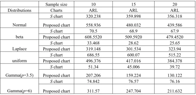
Table 3. In control ARL for S chart and the proposed control charts for different sample sizes and distributions.
Sample size 10 15 20
Distributions Charts ARL ARL ARL
S chart 320.238 359.898 356.318 Normal Proposed chart 558.936 480.032 439.586 S chart 70.5 68.9 67.9 beta Proposed chart 608.5520 509.5920 479.4520
S chart 33.468 28.62 25.65 Laplace Proposed chart 319.148 301.534 323.94
S chart 686.55 600.07 515.22 uniform Proposed chart 496.376 417.016 384.378
S chart 51.34 45.006 39.72 Gamma(p=3.5) Proposed chart 207.206 159.224 130.122
S chart 74.842 76.57 76.16 Gamma(p=6) Proposed chart 311.57 247.704 211.632
4. FINDINGS
• With respect to in control ARL performance, of the proposed method is uniformly better than the S chart for Normal, Laplace, Beta, Gamma (p=3.5) and Gamma (p=6). In case of uniform distribution the performance is poorer than S chart but it is acceptable.
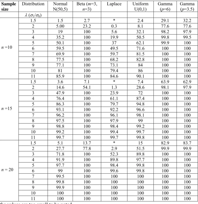
Table 4. Percent of correct classification to detect a shift in variability for the proposed control charts for different sample sizes and distributions.
Sample size
Distribution Normal
N(50,5) Beta (n=3) m=3, Laplace Uniform U(0,1) Gamma (p=6) Gamma (p=3.5) λ (σ1/σ0)
1.5 1.5 2.7 * 2.4 29.1 32.2
2 5.00 23.2 0.3 8.1 77.6 77.6
3 19 100 5.6 32.1 98.2 97.9
4 35.2 100 19.9 50.5 99.8 99.5
5 50.1 100 37 62.1 99.9 100
6 59.5 100 49.5 71.6 100 100
7 69.9 100 59.7 81.5 100 100
8 77.5 100 68.2 82.8 100 100
9 77.1 100 73.1 84 100 100
10 81 100 79.4 86 100 100
n =10
11 85.9 100 84.6 90.1 100 100
1.5 3.6 7.1 * 7.4 63.9 62.9
2 14.6 54.1 1.3 28.6 98.1 97.9
3 47.9 100 23.9 72 100 100
4 76.4 100 61.1 87.4 100 100
5 86.3 100 79.7 94.8 100 100
6 93.1 100 92.2 96.6 100 100
7 96.2 100 96.1 98.1 100 100
8 97.5 100 97.9 99 100 100
9 98.8 100 98.4 99.2 100 100
10 99.2 100 99.4 99.7 100 100
n =15
11 99.7 100 99.7 99.8 100 100
1.5 5.1 13.7 * 15 82.9 83.7
2 27.7 77.8 2.9 51.5 99.9 99.9
3 71.8 100 52.3 89.8 100 100
4 91.9 100 89.8 97.7 100 100
5 97.7 100 98.4 99.8 100 100
6 99 100 99.6 99.8 100 100
7 99.5 100 100 100 100 100
8 99.8 100 100 100 100 100
9 99.9 100 100 100 100 100
10 100 100 100 100 100 100
n = 20
11 100 100 100 100 100 100
* the values are too small to be noted.
It is worthwhile to note here that the values of λ≤ 1 are not considered. This is because of the fact thatλ = (σ1/σ0) and 1/λ = (σ0/σ1.). Hence P(σ1=λσ0) = P(σ0=σ1/λ). Consequently, the percent of
classification to detect a shift of 1/λ in variability, only the alternative hypothesis will change accordingly.
Furthermore, the out of control performance of the proposed chart can not be compared with that of
S chart since they are having significantly different in control ARL values. In this paper we are trying to convince the reader that in control performance of the proposed chart is much better than the corresponding S chart and its out of control performance is also remarkable. Especially, when the proposed chart is able to detect the shift in variability for more than 95% cases (and for some cases it attains 100%) there is no need to compare the performance with another chart.
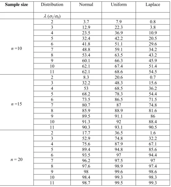
Additionally, if we consider the out of control performance of a parallel non-parametric control chart viz. the chart proposed by Das (2008) based on by Ansari and Bradley (1960) two sample variability test the proposed chart is showing better performance out of control % correct classification. Comparison of Table 4 and Table 5 support the statement.
Table 5. Percent of correct classification to detect a shift in variability for the control chart based on Ansari Bradley test for different sample sizes and distributions.
Sample size Distribution Normal Uniform Laplace λ (σ1/σ0)
2 3.7 7.9 0.8
3 12.9 22.3 3.8
4 23.5 36.9 10.9
5 32.4 42.2 20.5
6 41.8 51.1 29.6
7 48.8 59.1 34.2
8 53.4 63.5 43.2
9 60.1 66.3 45.9
10 62.1 67.4 51.4
n =10
11 62.1 68.6 54.5
2 8.3 20.6 0.7
3 32.2 48.3 15.6
4 53 68.5 36.2
5 68.2 78.3 54.4
6 73.5 86.5 71.5
7 80.7 87 74.8
8 85.9 88.9 81.6
9 89.5 91.1 86
10 91.3 92 88.4 n =15
11 90.3 93.1 90.5
2 17.7 36.5 1.6
3 52.9 74.8 32.2
4 75.6 87.9 67.1
5 89.4 94.8 85.6
6 93.5 97 94.4
7 96.2 97.5 97
8 97.6 98.9 97.4
9 98 99.6 98.6
10 98.4 99.3 98.3
n = 20
In general we can conclude the following:
• The performance of the proposed method is better than that proposed by Das (2008).
• With the increase of sample size the performance of each method is increasing to detect a particular shift.
• For almost all the distributions the performance of the proposed method to detect the shift, taking the sample size = 20, is highly encouraging.
• For sample size= 15 the performance of the method is quite good to detect the shift >5.
• For n=10, performance is poor for Gamma, moderate for Laplace but very good for normal and uniform.
5. SUMMARY AND CONCLUSIONS
• The proposed non-parametric control chart for dispersion shows that it’s performance is better than parametric S chart when in control ARL is considered for all distributions.
• As far as the performance to detect the shift in dispersion i.e., the power is concerned the proposed method is performing at par and better than a parallel nonparametric control chart for monitoring variability proposed by Das (2008) .
• Sample size greater than equal to 15 is recommendable.
• We have noticed a different picture in ‘in control’ and ‘out of control’ situations. To be precise, in control situation ARL decreases with the increase of sample size but in out of control situation % correct classification increases with the increase of sample size. This is expected since for any test of hypothesis if we try to increase probability of Type-I error (α) which is related to in control situation then probability of Type-II error (related to out of control situation) will decrease and vice versa.
REFERENCES
[1] Alloway J.A., Raghavachari M. (1991), Control Chart based on Hodges-Lehmann Estimator; Journal of quality Technology 23; 336-347.
[2] Altukife F.S. (2003), A New Nonparametric Control Charts Based on the Observations Exceeding the Grand Median; Pakistan Journal of Statistics 19(3); 343-351.
[3] Altukife F.S. (2003), Nonparametric Control Charts Based on Sum of Ranks; Pakistan Journal of Statistics 19(3); 291-300.
[4] Amin R.W., Reynolds M.R., Jr., baker S.T. (1995), Nonparametric Quality Control Charts Based on the Sign Statistic; Communications in Statistics-Theory and Methods 24; 1579-1623.
[5] Ansari A.R., Bradley R.A. (1960), Rank Sum Test for Dispersion; Annals of Mathematical Statistics 31; 1174-1189.
[6] Bakir S.T., Reynolds M.R, JR. (1979), A non Parametric Procedure for Process Control Based on within Group Ranking; Technometrics 21; 175-183.
[7] Bakir S.T. (2001), Classification of distribution free control charts; Proceedings of annual meeting of American Statistical Association Aug 5-9; Section Quality and Productivity.
[8] Bakir S.T. (2006), Distribution-Free Quality Control Charts Based on Signed Rank Like Statistics; Communications in Statistics, Theory and methods, 35; 743-757.
[9] Bhattacharya P.K., Frierson D.(1981), A Non-parametric control Control Chart for Detecting Small Disorders; Annals of Statistics 9; 544-554.
[10] Bradly J.V.(1968), Distribution-Free Statistical Tests; Prentice-Hall, New Jersy.
[11] Chakraborti S., Van der Lann P., Van de Wiel M.A. (2001), Nonparametric Control Charts: An Overview and Some Results; Journal of Quality Technology 33; 304-315.
[12] Conover W.J. (1980), Practical Nonparametric Statistics; John Wiley& Sons., New York.
[13] Das N. (2008), A Note on Efficiency of Non parametric Control chart for Monitoring Process variability; Economic Quality Control 23 (1); 85-93.
[14] Ferrell E.B. (1953), Control Charts using Midranges and Medians; Industrial Quality Control 9; 30-34. [15] Jacobs D.C. (1990), Statistical Process Control: Watch for Nonnormal Distributions; Chemical
Engineering Progress 86; 19-27.
[16] Kao, Ho (2006), Process monitoring of the sample variances through an optimal normalizing transformation; The International Journal of Advanced Manufacturing Technology 30(5-6); 459-469. [17] Kiani M., Panaretos J.,·Psarakis S. (2008), A new procedure for monitoring the range and standard
deviation of a quality characteristic; Quality and Quantity; DOI 10.1007/s11135-008-9175-x.
[18] Langenberg P., Iglewicz B. (1986), Trimmed Mean
X
andR
Charts; Journal of Quality Technology18; 152-161.[19] Lehmann E.L. (1975), Nonparametrics: Statistical Methods based on Ranks; Holden-Day., San Fransisco, California.
[20] Orban J., Wolfe D.A. (1982), A Class of Distribution-Free Two-Sample Tests Based on Placements; Journal of the American Statistical Association 77; 666-672.
[21] Park C., Reynolds M.R., Jr. (1987), Nonparametric Procedures for Monitoring a Location Parameter based on Linear Placement Statistics; Sequential Analysis 6; 303-323.
[22] Pappanastos E.A, Adams B.M. (1996), Alternative designs of the Hodges-Lehman Control Chart; Journal of Quality Technology 28; 213-223.
[23] Qiu P., Hawkins D.M. (2003), A nonparametric multivariate CUSUM procedure for detecting shifts in all directions; Statistician 52; 151-164.
[24] Riaz M. (2008), Monitoring process variability using auxiliary information; Computational Statistics 23(2); 253-276.
[25] Shewhart W.A. (1939), Statistical Methods from the Viewpoint Of Quality Control Republished in 1986 by Dover Publication; New York, NY.
[26] Sprent P. (1989), Applied Nonparametric Statistical Methods; Chapman & Hall, New York, NY. [27] Tukey J.W. (1960), A Survey of sampling from Contaminated Distributions. Contributions of
Probability and Statistics, Essay in Honor of Harold Hotelling. (I. Olkin et al., eds.); Stanford University Press, Stanford, CA.
[28] Willemain T.R., Runger G.C. (1996), Designing Control Charts Using an Emperical Reference Distribution; Journal of Quality Technology 28; 31-38.
[29] Wetherill G.B., Brown D.W. (1991), Statistical Process Control; Chapman and Hall, New York. [30] Woodall W.H. (2000), Controversies and Contradictions in Statistical Process Control;.Journal of
Quality Technology 32; 341-378.
[31] Woodall W.H., Montgomery D.C. (1999), Research Issues and Ideas in Statistical Process Control; Journal of Quality Technology 31; 376-386.
[32] Yourstone S.A., Zimmer W.J. (1992), Non-normality and the Design of Control Charts for Averages; Decision sciences 23; 1099-1113.
[33] Zhou C., Zhang Y., Wang Z. (2007), Nonparametric control chart based on change-point model; Statistical Papers.