Winter 2011
A Comprehensive Fuzzy Multiobjective Supplier Selection Model under
Price Brakes and Using Interval Comparison Matrices
Mehdi Seifbarghy1, Ali Pourebrahim Gilkalayeh2, Mehran Alidoost 3
1Technical and Engineering Department, Alzahra University, Tehran, Iran
2,3Faculty of Industrial and Mechanical Engineering, Islamic Azad University, Qazvin Branch, Qazvin, Iran 2[email protected], 3[email protected]
ABSTRACT
The research on supplier selection is abundant and the works usually only consider the critical success factors in the buyer–supplier relationship. However, the negative aspects of the buyer– supplier relationship must also be considered simultaneously. In this paper we propose a comprehensive model for ranking an arbitrary number of suppliers, selecting a number of them and allocating a quota of an order to them considering three objective functions: minimizing the net cost, minimizing the net rejected items and minimizing the net late deliveries. The two-stage logarithmic goal programming method for generating weights from interval comparison matrices (Wang et al. 2005) is used for ranking and selecting the suppliers. It is assumed that the suppliers give price discounts. A fuzzy multiobjective model is formulated in such a way as to consider imprecision of information. A numerical example is given to explain how the model is applied.
Keywords: Supplier Selection, Interval Comparison Matrices, Fuzzy Multiobjective Model, Price Discounts, Supply Chain.
1. INTRODUCTION
In today’s competitive environment making products with high quality and low cost is impossible without accessing qualified suppliers. Selecting a qualified supplier is also a key step in making successful alliances. Supplier selection problem is a very important task in procurement management. It could be a time consuming function in many competitive businesses. Having selected qualified suppliers could guarantee the high quality and service level and also robust relationships with the selected suppliers. Having several suppliers decreases the supply risk but simultanously increases the supply cost and complexity. Numerous studies have been carried out on determining key criteria of suppliers’ evaluation. In order to manage the suppliers, vendors usually divide their suppliers into two categories. The first is the category of suppliers which are strategic for the vendor and the second is the category of suppliers which are not strategic. The criteria considered for evaluating each category are different. Strategic suppliers are those which supply the key parts of the final product.
Corresponding Author
Supplier evaluation and selection is a multi-criteria problem and is usually treated using Multiple Criteria Decision Making (MCDM) techniques. MCDM techniques help the Decision Maker (DM) in evaluating various suppliers subject to some criteria. Based on the purchasing conditions, the criteria might be of different importance. In many cases the suppliers offer some types of discounts and the vendor should determine the amount of purchase from each supplier. This is a Multi Objective Decision Making (MODM) problem with conflicting objectives. Supplier (vendor) selection problem has been considered as a complex problem in the literature due to several reasons (Kumar et al. 2006):
(i) Selected vendors need to be evaluated on more than one criterion. Dickson (1966) identified criteria for vendor selection, while Dempsey (1978) describes 18 criteria. In a review of 74 articles Weber et al. (1991) concludes that by nature vendor selection is a multiple objective problem.
(ii) Individual vendors may have different performance characteristics for different criteria. (iii) Constraints related to vendors’ internal policy and externally imposed system constraints of
the supply chain put restrictions on vendors’ quota allocation, number of vendors to employ, minimum and maximum order quantities, use of minimum number of vendors, etc. (iv) Suppliers may impose constraints on the supplying process so as to meet their own
minimum order quantities or maximum order quantities which may be based on their production capacity.
(v) There may be time constraints on the delivery of items. Within these time constraints, some criteria supplying the items may become important, while other criteria may not be the dominant ones.
In many applications, due to incomplete information and knowledge, unquantifiable information, imprecise data, etc., a natural way for expressing preferences is interval assessments (Dopazo (2009)).
In this paper we extend Amy and Lee. I (2008) tweleve-stage model which is based on Saaty (2003, 2004) and Lee. (2009). In the addressed research a systematic simple fuzzy AHP model is proposed for ranking the suppliers and quota allocation. The extensions in this paper are: first, applying the two-stage logarithmic goal programming method for generating weights from interval comparison matrices of Wang et al. (2005) while performing the pairwise comparisons which is more practical and precise than that of Amy and Lee (2008); second, applying the fuzzy multiobjective model under price breaks (Amid et al. (2008)) for quota allocation problem which makes it possible to consider different prices of vendors for different levels in the model and also to formulate the problem as a mathematical programming with optimal solutions. In other word this paper proposes a comprehensive model for ranking an arbitrary number of suppliers, selecting a number of them and assigning a total order quantity to them considering three objective functions: minimizing the net cost, minimizing the net rejected items and minimizing the net late deliveries. The two-stage logarithmic goal programming method for generating weights from interval comparison matrices (Wang et al. 2005) is used for ranking and selecting the suppliers. It is assumed that the suppliers give price discounts. A fuzzy multiobjective model is formulated in such a way as to consider imprecision of information. A numerical example is given to explain how the model is applied. The paper is structures as follows: Section 2 gives a brief literature review. In Section 3, we review the concept of the interval comparisons and the degree of preferences. Section 4 gives the proposed
model for supplier selection and quota allocation. In Ssection 5 a case study is solved based on the proposed model and the paper is concluded in Section 6 with conlusion and further research.
2. LITERATURE REVIEW
In this section we first review researches devoted to proposing criteria on vendor selection, then we review mathematical programming models which mostly emphasize on quota allocation to selected vendors and finally we review one of the major techniques used in this paper titled ―interval comparison matrices‖ while ranking the vendors in order to select the qualified ones.
Until recent years, the literature on vendor selection had been mainly qualitative and focused primarily on methodological aspects. Selecting qualified suppliers, Geringer (1988) introduced some criteria such as financial assets, managerial experience and access to markets, and the partner’s national culture, past experience, size and structure. Lewis (1990) proposed a qualitative approach to model the supply chain partner selection problem. Several criteria were suggested, such as value added to products, operations and technologies strengthening and improvement in market access to evaluate suppliers. Lorange et al. (1992) developed a two-stage supply chain selection approach. The first stage is to evaluate the matching degree with candidate partners. The second stage is to analyze the market potential, main competitors and the worst-case scenarios simulation after the relationship formation. Narasimahn (1983), Nydick and Hill (1992) and Partovi et al. (1989) were the earliest researches which adopted Analytic Hierarchy Process (AHP) for supplier selection problems. The major reasons for applying AHP are its capability of handling both qualitative and quantitative criteria and being easily understood and applied by people. Mikhailov (2002) presented a fuzzy approach for partnership selection problem in the formation of virtual enterprises. Lin and Chen (2004) identified 183 decision attributes for evaluating candidate supply chain alliances for general industries.These attributes are further categorized such as finance, human resource management, industrial characteristics, knowledge/technology acquiring and management, marketing, organizational competitiveness, product development, production, and logistics management, and relationship building.
Mathematical Programming (MP) models on supplier (vendor) selection problem can be subdivided into Linear Programming (LP), Mixed Integer Programming (MIP), and goal programming/Multi-Objective Programming (MOP). Some researches which use MP models are reviewed in Muralidharan et al. (2002), Weber et al. (1998) and Weber and Desai (1996). Kaslingam and Lee (1996) developed an MIP model to select suppliers and to determine order quantities with the objective of minimizing total supplying costs which include purchasing and transportation costs. Weber and Current (1993) introduced an MOP for selecting suppliers and determining order quantities considering multiple conflicting criteria. Weber and Desai (1996) applied Data Envelopment Analysis (DEA) in supplier evaluation for an individual product and discussed the advantages of applying DEA. Ghodsypour and O’Brien (1998) proposed an integrated method which used AHP and LP to choose the best supplier and to assign the optimum order quantity among selected suppliers. Weber et al. (1998) combined MOP and DEA to evaluate suppliers. Hong, Park, Jang, and Rho (2005) proposed a mathematical programming model which considers the change in supply capabilities and customer needs over a period of time, the model not only can maximize revenue but also can satisfy customer needs.
Liu and Hai (2005) proposed a method which combined AHP and DEA for selecting suppliers. Kumar et al. (2004) formulated a vendor selection problem as a fuzzy mixed integer goal programming model which included three primary objectives, minimizing the net cost, minimizing
the net rejections and minimizing the net late deliveries subject to constraints including buyer’s demand, vendors’ capacity, vendors’ quota flexibility, purchase value of items and budget allocation to individual vendor. Kumar et al. (2006) further developed a fuzzy multi-objective integer programming approach for vendor selection problem in a supply chain. Amid et al. (2006) also formulated a supplier selection problem in a supply chain by establishing a fuzzy multi-objective linear model applying an asymmetric fuzzy-decisionmaking technique. Wu et al. (2010) proposed a fuzzy multi-objective programming model to decide on supplier selection in a three level supply chain. They considered risk factors and used simulated historical quantitative and qualitative data. They proposed a possibility approach to solve this model. Ravindran et al. (2010) developed multicriteria supplier selection models incorporating supplier risk and applied them to a global company. For solving this problem, they first reduced a large set of initial suppliers to a smaller set of manageable suppliers using various multi-objective ranking methods. Then, they allocated order quantities among the short listed suppliers using a multi-objective optimisation model.
The interval comparison matrix has been of great attention in the recent researches. Van Laarhoven and Pedryce (1983) considered treating elements in a comparison matrix as fuzzy numbers having triangular membership functions and employed the logarithmic least-squares method to generate fuzzy weights. Buckley (1985) extended the method to trapezoidal membership functions and hierarchical analysis. Boender et al. (1989) found a fallacy in the normalization procedure of Van Laarhoven and Pedryce’s method for generating fuzzy weights and subsequently modified the method. Xu and Zhai (1996) discussed the problem of extracting fuzzy weights from a fuzzy judgment matrix as well as using the logarithmic least-squares method based on a distance definition in a fuzzy judgment space. Xu (2000) used the same distance definition to develop a fuzzy least-squares priority method. Leung and Cao (2000) proposed a fuzzy consistency definition considering a tolerance deviation and determined fuzzy local and global weights using the extension principle. Buckley et al. (2001) directly fuzzified Saaty’s original procedure of computing weights in hierarchical analysis to get fuzzy weights in the fuzzy hierarchical analysis. Csutora and Buckley (2001) presented a Lambda–Max method to find fuzzy weights. Wang and chin (2006) proposed an eigenvector method (EM) to generate interval or fuzzy weight estimation from an interval or fuzzy comparison matrix, which differed from Csutora and Buckley’s Lambda-Max method in several aspects. First, the proposed EM produced a normalized interval or fuzzy eigenvector weight estimation through the solution of a linear programming model. Second, the EM directly solved the principal right eigenvector of an interval or fuzzy comparison matrix. Finally, the Lambda-Max method applied the principal right eigenvector of a crisp comparison matrix to determine the final interval weights. Dopazo et al.(2007) focued on the problem of learning the overall preference weights of a set of alternatives from the (possibly conflicting) uncertain and imprecise information given by a group of experts into the form of interval pairwise comparison matrices and proposed a two-stage method in a distance-based framework, where the impact of the data certainty degree was captured.
Saaty and Vargas (1987) proposed interval judgments for AHP method as a way to model subjective uncertainty and used a Monte Carlo simulation approach to find out weight intervals from interval comparison matrices. They also pointed out difficulties in using this approach. Arbel (1989, 1991) interpreted interval judgments as linear constraints on local priorities and formulated the prioritization process as a LP model. Kress (1991) found that Arbel’s method is ineffective for inconsistent interval comparison matrices because no feasible region exists in such circumstances. Salo and Hämäläinen (1992, 1995) extended Arbel’s approach to hierarchical structures. Their method found the maximum and minimum feasible values for all interval priorities and incorporated the resulting intervals into further synthesis of global interval priorities. Arbel and
Vargas (1990, 1993) formulated the hierarchical problem as a nonlinear programming model in which all local priorities in a hierarchy are included as decision variables and also established a connection between Monte Carlo simulation and Arbel’s LP approach. Moreno-Jiménez (1993) studied the probability distribution of possible rankings of the alternatives in an interval comparison matrix of size n = 2 or 3. Islame et al. (1997) used a Lexicographic Goal Programming (LGP) technique to find out weights from inconsistent interval comparison matrices and explored its properties and advantages as a weight estimation technique. Haines (1998) proposed a statistical approach to extract preferences from interval comparison matrices. Two specific distributions on a feasible region were examined and the mean of the distributions was used as a basis for assessment and ranking. Mikhailov (2002, 2003, 2004) developed a Fuzzy Preference Programming (FPP) method to derive crisp preferences from interval or fuzzy comparison matrices and extended the method to the case of group decision making. Dopazo and Ruiz (2009) developed methods for the estimation of punctual priority weights from interval pairwise comparison matrices given by a group of experts. The development of the addressed methods relied on lp-distances to measure the distance between the preference information given by the experts and its normative prototype. Then a minimization problem in the l p-distance under some constraints was obtained. The proposed approach became operational using an interval goal programming formulation. Conde and Paz Rivera (2010) proposed a decision making model to assess a finite number of alternatives according to interval judgement matrix. They analyzed the problem of determination of an efficient solution using a multi-objective optimization problem.
The literature review shows that only Monte Carlo simulation, LGP and FPP methods could be used to generate weights from both consistent and inconsistent interval comparison matrices. All the other existing methods mentioned above are only applicable to consistent interval comparison matrices. As pointed out by Saaty and Vargas (1987), Monte Carlo simulation is rather complicated and time consuming in computation. Since the number of simulations is always limited, the accuracy of the resultant priority intervals may not be satisfactory. In general, weight intervals generated by Monte Carlo simulations are narrower than the real priority intervals. Although Islame et al’s LGP and Mikhailov’s FPP methods can both be used to generate weights from inconsistent interval comparison matrices, the former is defective in theory because using the upper or lower triangular judgments of an interval comparison matrix could always lead to different priority rankings, the latter requires the DM to predetermine the values of all tolerance parameters and both methods can only generate a crisp set of priorities in the presence of inconsistency. Since judgments in an interval comparison matrix are imprecise, it is more natural and logical generating an interval weight vector than generating an exact priority vector that is only a point estimate. However, how to generate a valid estimate for weighs in the presence of inconsistent interval comparison matrices and how to develop an effective method that is applicable to both consistent and inconsistent interval comparison matrices still remains unsolved.
3. THE INTERVAL COMPARISON MATRICE AND DEGREE OF PREFERENCES
Suppose the decision maker provides interval judgments instead of precise judgments for a pairwise comparison. For example, it could be judged that criterion i is between lijand uijtimes as important as criterion j with lijand uijbeing nonnegative real numbers and lijuij. Then, an interval comparison matrix can be represented by (Wang et al. 2005):
12 12 1 1
21 21 2 2
1 1 2 2
1
[
,
]
[
,
]
[
,
]
1
[
,
]
(
)
[
,
] [
,
]
1
n n
n n ij n n
n n n n
l
u
l
u
l
u
l
u
A
a
l
u
l
u
(1)
where lij 1/uijand uij 1/lijand lij aij uij.
The matrix could be the interval comparison matrix of some criteria or alternatives. Wang et al. (2005) gives the definition of consistent and inconsistent interval comparison matrix and after giving some theorems and proofs, concludes that the weights of each criterion i, assuming the matrix to be the interval comparison of criteria, namely
[
w w
il iu]
is obtained from solving thefollowing mathematical programming ((2)-(8)). wil is obtained from the objectice function while minimizing it and wiu is obtained from the objective function while maximizing the objective function.
Min/Max ln
w
i
x
i
y
i (2)Subject to
ln , 1,..., 1, 1,..., ,
i i j j ij ij
x y x y p l i n j i n (3)
ln
,
1,...,
1,
1,..., ,
i i j j ij ij
x
y
x
y
q
u
i
n
j
i
n
(4)1
(
)
0,
n
i i i
x
y
(5)1
* 1 1
(
)
,
n n
ij ij i j i
p
q
J
(6),
0,
0,
1,..., ,
i i i i
x
y
x y
i
n
(7), 0, 0, 1,..., 1, 1,...,
ij ij ij ij
p q p q i n j i n. (8)
Where
J
* is the optimium value of the following mathematical programming objective function.1 1 1
Min
(
)
n n
ij ij i j i
J
p
q
(9)Subject to
ln , 1, , 1, 1, , ,
i i j j ij ij
x y x y p l i n j i n (10)
ln , 1, , 1, 1, , ,
i i j j ij ij
x y x y q u i n j i n (11)
1
(
)
0,
n
i i i
x
y
,
0,
0,
1,
, ,
i i i i
x
y
x y
i
n
(13), 0, 0, 1, , 1, 1, ,
ij ij ij ij
p q p q i n j i n (14)
If the matrix A to be the interval comparison matrix of the alternatives, the same procedure as (2)-(14) should be done to obtain
[
w w
ijl iju]
which is the interval weight of each alternative j with respect to the criterion i (i1,...,n and j1,...,m )Let
a
[ ,
a a
1 2]
andb
[ , ]
b b
1 2 be two interval weights, Wang et al. (2005) also defines the degreeof preference of an over b as (15) and inversely the degree of preference of b over a as (16). The degree of preference is referd to the degree of one interval weight being greater than another.
2 1 1 2
2 1 2 1
max(0, ) max(0, )
( )
( ) ( )
a b a b
P a b
a a b b
(15)
2 1 1 2
2 1 2 1
max(0, ) max(0, )
( )
( ) ( )
b a b a
P b a
a a b b
(16)
4. MODEL PRESENTATION
A two-phase model is proposed in order to ranking and selecting the qualified suppliers and allocating quota to each supplier. The reason why using the proposed method is the hierarchical structure of the problem as well as the differences in the expert’s judjments. At the first phase the regular comparison matrices are converted to the interval comparison matrices and then using the two-stage logarithmic goal programming method of Wang et al. (2005), the criteria and their subcriteria are weighted and the alternatives are ranked respect to the criteria. At the second phase the quota of each supplier is determined considering the fuzzy demand constraint and the three fuzzy objectives regarding to cost, rejected items and delayed deliveries. It should be noted that each supplier has a few discount points which is considered in the proposed model. The addressed phases are explained in details.
Phase 1: Ranking and selecting the qualified suppliers
1. Form a committee of experts in the industry and define the supplier selection problem.
2. Make a hierarchy of benefits, costs, opportunities and threats using the experts. Determine the criteria and subcriteria for each and complete the hierarchy. The lowest level of the hierarchy should include the alternatives which are suppliers here.
3. Perform the pairwise comparisons for the criteria, subcriteria and alternatives using the experts. 4. Form the interval comparison matrices. In this step having gathered the experts’ judgments, the upper and lower bounds of the interval are equal to the maximum and the minimum amounts of the judgments. For example if there is considered three experts with given numbers of 2, 2 and 3 in a pairwise comparison of two items, the lower and bounds of the interval are equal to 2 and 3 respectively.
5. Consider the consistency of the interval comparison matrices. This is done by solving the mathematical programming model proposed by Wang et al. (2005) which is given as (9)-(14). If the objective function value becomes zero the corresponding interval comparison matrice is consistent otherwise it is inconsistent however (9)-(14) tries to minimize the inconsistency…. In (9)-(14)
ij
p and qijare both nonnegative real numbers, but only one of them can be positive since pij.qij 0.
For consistent judgments, both pijand qijare zero and J 0. In the presence of inconsistent judgments, only one of pijand qijmay be unequal to zero. (9)-(14) holds for both consistent and inconsistent judgments. It is desirable that the deviation variables pijand qijare kept to be as small as possible, which means to minimize the inconsistency of interval comparison matrices. The optimal value of the objective function is named
J
*.6. Calculate the interval weights of criteria, subcriteria and alternatives. In this step we may come across two cases: The first one is that the corresponding matrix is inconsistent which meansJ*0.
In order to find the interval weights as mentioned in Section 3, we solve the mathematical programming model as (2)-(8). The second one is that the corresponding matrix is consistent which meansJ*0. In this case the as Wang et al. (2005) the following mathematical programming
model should be solved..
Min/Max ln
w
i
x
i
y
i (17)Subject to
ln , 1, , 1, 1, , ,
i i j j ij
x y x y l i n j i n (18)
ln , 1, , 1, 1, , ,
i i j j ij
x y x y u i n j i n (19)
1
(
)
0,
n i i i
x
y
(20),
0,
0,
1,
, .
i i i i
x
y
x y
i
n
(21)7. Calculate the ultimate weights of the criteria, subcriteria and alternatives. As Wang et al. (2005) suppose interval weights for upper-level criteria and lower-level alternatives have all been obtained, as shown in Table 1, where [w wil iu]is the interval weight of criterion j (j = 1, . . . , m) and
] ,
[ Uij
L ij w
w is the interval weight of alternative
A
i with respect to the criterion j (i = 1, . . . , n; j = 1, . . . ,m).Table 1 Synthesis of interval weights
Composit Weights Criterion m Criterion 2 Criterion 1 Choices ] ,
[ Um
L m w w ] , [w2L w2U ]
, [w1L w1U
] , [ 1 1 U A L A w w ] , [w1Lm w1Um
] , [w12L w12U ]
, [w11L w11U 1 A ] , [ 2 2 U A L A w w ] , [w2Lm wU2m
] , [w22L wU22 ]
, [w21L w21U 2 A ] ,
[ UA
L An w n
w ] , [wnmL wUnm
] , [wnL2 wUn2 ]
, [wnL1 wUn1
n
As Wang et al. (2005) the following pairs of nonlinear programming models are suggested for the synthesis of interval weights:
1
( ) j
i ij
m w
L L
A j
Minw w
(22)Subject to
,
W
W (23)
1
( ) j
i ij
m w
U U
A j
Max w w
(24)Subject to W
W (25)
Where W(w1,...,wm) and
m
i j U
j j L j m
w W w w w w w w
1
1,..., )| , 1
( and U
Ai
w and U Ai
w are, respectively, the lower and upper bounds of the composite weight
i
A
w , which constitute aninterval
denoted by
U
A L A Ai w i w i
w , (
i
1,...,
n
). The global interval weight for each alternative can begenerated by repeating the above synthesis processes until reaching the top level, which represents thegoal of decision analysis.
8. Calculate the relative degree of preferences of the alternatives to eachother as (15) and (16). 9. Rank and select the qualified alternatives. Clculate the sume of relative degree of preferences for each alternative and rank them. We can select the qualified suppliers which are of higher ranking.
Phase 2: Allocate the quota to each selected supplier
10. Make the following multiobjective model.
In this step the problem of determining each supplier’s qiota is formulated as a multi objective integer programming. The objectives are minimizing the cost, delayed deliveries and rejected units. A model considering price discounts is presented. The parameters and variables are as following:
ij
x : The number of units purchased from the ith supplier at price level j ij
P : Price of the ith supplier at level j ij
V : Maximum purchased volume from the ith supplier at jth price level
ij
V : Slightly less than Vij D: Demand over the period
i
i
m : Number of price level of the ith supplier i
F : Percentage of items delivered late for the ith supplier i
S : Percentage of rejected units for the ith supplier i
x
: Order quantity of the ith supplier) ( i
i x
P : Price a buyer must pay to supplier i for supplying the order quantity
x
i n: Number of suppliers0 0
1 0
ij ij
ij
if x Y
if x
Consider a buyer whose demand is D units of a particular product over a fixed planning period.
Thus: x D
n
i i
1.
Each supplier has a known capacity and can replenish less than or equal to its capacity. The final form of the mixed integer multiobjective linear model for purchasing a single item in multiple sourcing network ia as follows (The model is rather close to Amid et al. (2008) and the difference is that we should certainly purchase from all the seleted suppliers):
1
1 1
i
m n
ij ij i j
Min Z P x
(26)2
1 1
i
m n
i ij
i j
Min Z S x
(27)3
1 1
i
m n
i ij
i j
Min Z F x
(28)Subject to
1 1
i
m n
ij i j
x D
(29)1
, 1, 2,...,
i
m
ij i j
x C i n
(30), 1, , 1, 2,..., ; 1, 2,...,
i j ij ij i
V Y x i n j m (31)
, 1, 2,..., ; 1, 2,...,
ij ij ij i
V Y x i n j m (32)
1
1, 1,...,
i
m ij j
y i n
(33), 0,1, 1, 2,..., ; 1, 2,...,
i j i
0, 1, 2,..., ; 1, 2,..., .
ij i
x i n j m (35)
The objective function in Equation (26) minimizes the purchasing cost and in Equation (27) minimizes the return orders and in Equation (28) minimizes the delayed deliveries.
Constraint (29) implies that the sume of all units purchased from the suppliers at all corresponding price levels, should be equal to the demand. Constraint (30) implies that all units replenished from a supplier, should be less than or equal to the supplier replenishing capacity. Constraint (31) and (32) guarantee that in case of purchasing from supplier i at price level j, the amount of units should be in the corresponding discount interval. Constraint (33) implies that one price level per supplier can be chosen. Constraint (34) and (35) implies that
Y
ij must be integer and xij must not be negative. 11. Fuzzifying the modelThe objective functions and the demand related constraint are fuzzyfied. The resulting model can be stated as (Amid et al. (2008)):
1 1
1 1
~
i
m n
o ij ij i j
Min Z P x Z
(36)2 2
1 1
~
i
m n
o i ij i j
Min Z S x Z
(37)3 3
1 1
~
i
m n
o i ij i j
Min Z F x Z
(38)Subject to
1 1
i
m n
ij i j
x D
(39)o k
Z (k1,2,3) is the aspiration level for objective Zk that the DM wants to reach. 12. Defuzzification of the model
In a multi-objective problem in the context of fuzzy objectives, the approximate optimization of the objective functions is aimed. The approximate optimization of the objectives means that the membership function of each objective should be maximized. To obtain the membership functions of each objective, the objective function should individually be maximized and minimized subject to the exsiting constraints. We name Zkminas the minimum value of the objective function k th and
max k
Z as the maximum value of the objective function k th. The linear membership function of the objective function k th is as follows (Zimmerman (1978)):
min
max max min min max
max
1
( )
( )
[
( )] [
]
( )
0
( )
k z k
k k
Z k k k k k k k
k k
if
Z
x
Z
x
f
Z
Z
x
Z
Z
if
Z
Z
x
Z
if
Z
x
Z
The linear membership function for fuzzy constraints (less than or equal constraints) is obtained from dividing the difference of upper limit and the constraint function by the tolerance of the constraint and is stated as follows (Zimmerman (1978)):
1
( )( ) 1 ( ( ) ) ( )
0 ( )
gl
l l
gl l l l l l l l
l l l
if g x b
x f g x b d if b g x b d
if g x b d
(41)
In (41)
b
l andd
l are the upper limit and the mentioned tolerance.g x
l( )
is theconstraint function. In order to reach the crisp model, the membership function of each objective function is assumed to be greater than k which should be increased as much as possible. The membership function of the constraint is assumed to be greater than lwhich should be maximized. The crisp model is as in (42)-(46).1 1
P h
k k l l
k l
Max w
(42)
Subject to
, 1,...,
z k
k f k P
(43)
, 1,...,
gl
l f l h
(44)
1 1
1, 0 , 1
P h
k l k l
k l
w w
(45)
, 0,1
k l
(46)
Where wkand l are the weighting coefficients that present the relative importance among the fuzzy goals and constraints.
5. CASE STUDY
In this section we bring up an example to present the performance of the proposed model. In this example a car manufacturer is going to select two suppliers from six potential suppliers and to allocate the quota of each supplier from a total order. The management of the manufacturer candidates three experts to evaluate the suppliers. The criteria, sub-criteria and detailed criteria for evaluation are as in Table 2.
Then the experts make pairwise comparisons. The first one is for the criteria. Table 3 gives the results.
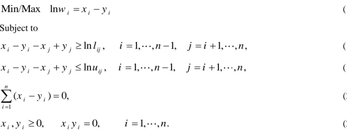
Such comparisons are made for sub-criteria and detailed criteria and the suppliers as the alternatives. Then the interval pairwise comparison matrix is obtained from combining the three expert’s results. Table 4 gives the results for just criteria.
Table 2 Criteria, sub-criteria and detailed criteria (Amy and Lee (2008)) Definitions Detailed criteria
sub-criteria criteria
The capability to provide quality products Yield rate
Quality (1-1)
Benefits (1)
The consistent conformance to specifications; quality stability Product reliability
The quality in providing support services, such as purchasing, technology support, etc. Quality of support services
The presence of good quality systems and continuous improvement programs Quality systems
Flexibility (1-2)
The ability to adjust product volume as demanded by the buyer
Volume flexibility
The ability to adjust product mix as demanded by the buyer
Product mix flexibility
The ability to customize product as demanded by the buyer
Customization
The ability to adjust manufacturing process as demanded by the buyer
Process flexibility
The ability to fill emergency orders with required amount in a required time Emergency order
processing
The ability to provide flexible services other than the above items
Flexibility in service
The duration of time from setting an order to the receipt of the order
Order lead time Delivery
(1-3)
The ability to follow the predefined delivery schedule
On time delivery
The consistency in meeting delivery deadlines
Delivery reliability
The quality and service of delivering products
Distribution network quality
The working records of the personel in the similar working areas inside company Personel records
Related records
(1-4) The working records in the area of parts supply in other companies
Similar Experience
The presence of an excellent technological system that can facilitate technology development of products
Technological system Supplier’s
technology (2-1)
Opportunities (2)
The expected technology development of products in the near future
Future technology development
The expected development of manufacturing capabilities in the near future
Future manufacturing capabilities
The possibility of reducing manufacturing costs
Cost-reduction capability
Buyer’s ability to acquire and secure critical knowledge and technologies from the supplier
Acquisition of supplier’s knowledge and
Technology Joint growth
(2-2)
The ability of the buyer and the supplier to complement each other’s capabilities Complementarities of
capabilities
The ability to jointly develop product and technology by both the buyer and the supplier
Joint product/technology development
The ability to maintain a long-term, stabilized relationship between the buyer and the supplier
Stabilized relationship Relationship
building (2-3)
Definitions Detailed criteria
sub-criteria criteria
The condition of current relationship and expected closeness between the buyer and the supplier
Closeness of relationship
The ability to maintain a good communication channel and negotiability with the supplier
Ease of communication
The purchase cost of materials Product price
Cost of product
(3-1) Costs
(3)
The transportation cost, inventory cost, handling and package cost, damages during transportation, and insurance costs
Freight cost
The extra processing cost, maintenance cost, warranty cost, and other costs related to the manufacturing of the product when using the material provided by the supplier
Extra cost
The cost to form a satisfactory buyer– supplier relationship, including financial cost, human resources, and coordinating and controlling costs
Cost of forming the relationship Cost of
relationship (3-2)
The duration of time required to form a satisfactory buyer–supplier relationship Time to forming the
relationship
The production facility and capacity constraint of the supplier
Supplier’s capacity limit Supply
constraint (4-1)
Risks (4)
The technology and production capability constraint in developing and producing a new product
Supplier’s capability limit
The difficulties of the supplier in obtaining required raw materials from its suppliers in the right quantity, in the specified quality, at the right time
Supplier’s raw material acquisition
Difficulties
The possibility of having an unstable, increasing-trend product price in compared with other suppliers in the future
Variation in price Buyer-
supplier Constraint
(4-2)
The degree of bargaining power of the supplier that may have an adverse impact on the buyer in terms of price, product specification, process specification, and so on, in the future
Bargaining power of supplier
Different management styles and organization cultures between the buyer and the supplier
Incompatibility between buyer and
Supplier
Supplier’s probable unsafe financial conditions (such as liquidity) and financial instability (e.g., whether the supplier involves in other risky businesses)
Financial risk Supplier’s
profile (4-3)
The unsatisfactory performance of the supplier in its past competitive nature, production results, and response to market, etc.
Bad performance history and reputation
Insufficient environmental controls and programs that may lead to unacceptable products for exporting to certain countries Inadequate environmental
controls and Programs
Table 3 The pairwise comparisons for criteria Third Expert Second Expert First Expert R C O B R C O B R C O B 5 3 3 1 3 2 2 1 3 3 2 1 Benefits 3 1/2 1 2 ½ 1 2 1/3 1 Opportunities 4 1 3 1 3 1 Costs 1 1 1 Risks
Table 4 Interval comparison matrix for the criteria Risks Costs
Opportunities Benefits
[3 5] [2 3]
[2 3] 1
Benefits
[2 3] [1/3 ½] 1
Opportunities
[3 4] 1
Costs
1 Risks
Now the consistency is considered. For this, (9)-(14) and (17)-(21) (if needed) is used. The results show that the matrix is consistent relations (22)-(25) is employed for calculating and obtaining the interval weights of the criteria are in Table 5.
Table 5 Criteria interval weights
Risks Costs Opportunities Benefits Criteria [0.3976, 0.4204] [1.5904, 1.6817] [0.7952, 0.8409] [1.6817, 1.9883] Interval weight
The consistency of all the interval comparison matrices is considered and the interval weights are determined for sub-criteria, detailed criteria and also for the suppliers as alternatives with respect to each detailed criteria. The interval weights are combined from the lowest level to uppest level and the final weights of the suppliers is obtained. At first step the interval weights of the suppliers with respect to the detailed criteria are determined and combined with the detailed criteria weights giving the suppliers interval weights with respect to sub-criteria. At the second step, the interval weights of the suppliers with respect to the sub-criteria are comined with the sub-criteria weights and give the suppliers interval weights with respect to the criteria. In this section and because of the high volume of the matrices, the interval weights of the supply constraint as sub-criteria is given as in Table 6.
Table 6 Supply constraint’s interval weights
Supply constraint Interval weights Detailed criteria
Alternative Supplier’s raw material
acquisition difficulties 0.5503] [0.3984 Supplier’s capability limit 2.1543] [1.4422 Supplier’s capacity limit 1.5873] [1 4.5398] [2.2004 1.2599] [1.2009 1.3730] [1.1936 1.7470] [1.4422 1 0.5339] [0.1239 0.8005] [0.6299 0.4163] [0.3779 1.5873] [1.2490 2 0.4106] [0.1528 1.2599] [1.2009 0.8326] [0.7558 0.5043] [0.3968 3 4.4299] [1.7090 2.5196] [2.4017 1.6652] [1.1517 0.9614] [0.7565 4 15.8681] [4.3611 0.6299] [0.6004 2.8175] [2.4494 1.7470] [1.4422 5 0.3394] [0.1269 0.6299] [0.6004 0.6614] [0.5359 0.8326] [0.6552 6
Combining all the interval weights, the interval weights of the suppliers are determined as in Table 7.
Table 7 Interval weights of the suppliers Interval weight Alternative
[345290 2.19E+18] 1
[6.1E-11 2.2E+13] 2
[2.7E-10 42388.4] 3
[2.4E-12 2496574] 4
[2.4E-12 12829400] 5
[1E-13 51523.85] 6
Using (15) and (16) we can obtain the degree of preferences of the suppliers. The results are given in Table 8. The ranking of the suppliers is given in Table 9.
Table 8 The degree of preerences the suppliers
Total 6 5 4 3 2 1 4.9999 1 1 1 1 0.9999 ---- 1 4 1 0.99999 1 1 ---- 0.00001 2 0.4713 0.4513 0.0032 0.0166 ---- 0 0 3 2.1259 0.9797 0.1628 ---- 0.9833 0 0 4 2.8298 0.996 ---- 0.8371 0.9967 0 0 5 0.5728 ---- 0.004 0.0202 0.5486 0 0 6
Table 9 The ranking of the suppliers
6 5 4 3 2 1 Suppliers 5 3 4 6 2 1 Alternatives rank
As the results in Table 9, the suppliers 1 and 2 are selected. In the next step the quota of each supplier should be determined. Table 10 gives the price break points, the percentage of returned units, delayed deliveries and the capacities for the selected suppliers. Demand is assumed as a triangle fuzzy number (16000 17000 18000)
Table 10 Selected suppliers information on the orders
Order level Price Return items Delayed deliveries Capacity Supplier 6000 Q 1000000 10% 10% 16000
1 950000 6000Q10000
10000 Q 910000 7000 Q 1000000 15% 20% 15000
2 950000 7000Q10000
10000 Q 940000
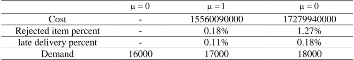
Now the upper and lower bounds of each objective function should be calculated individually subject to the constraints in order to obtain the membership functions. The results are given in Table 11.
Table 11 Requied information for membership functions 0 1 0 17279940000 15560090000 - Cost 1.27% 0.18% - Rejected item percent
0.18% 0.11%
- late delivery percent
18000 17000
16000 Demand
The corresponding fuzzyfied multi-objective model for this example can be stated as (47). It shoulg be noted that in order to obtain the lower and upper bound, we have used the crisp case of this model.
max
1 11 12 13 21 22 23 1
max
2 11 12 13 21 22 23 2
max 3 11 12 13 21 22 23 3 11 12 13 21 22 23
11 12 13
100000 950000 910000 100000 950000 940000
0.1( ) 0.15 ( )
0.1( ) 0.2 ( )
17000
Z x x x x x x Z
Z x x x x x x Z
Z x x x x x x Z
x x x x x x x x x
21 22 23 11 11 12 12 12 12 13 13 13 13 21 21 22 22 22 22 23 23 23 23
11 12 13 21 22 23
16000 15000 5999 0 6000 0 9999 0 10000 0 15999 0 6999 0 7000 0 9999 0 10000 0 14999 0 1 1 0 ,1 1, 2 , 1, 2 ij
x x x
x Y Y x x Y Y x x Y x Y Y x x Y Y x x Y
Y Y Y Y Y Y
Y i j
,...,
0, 1, 2 , 1, 2,..., i
ij i
m x i j m
(47)
Here the above model is converted to a crisp model using step 12 of the proposed method. In this example the weights of the three objectives and the constraint have been considered as 0.51, 0.26, 0.13 and 0.1 respectively as the expert’s judgments.
1 2 3
1 11 12 13 21 22 23
2 11 12 13 21 22 23
3 11 12 13 2
0.51 0.26 0.13 0.1 .
(17279940000 (100000 950000 910000 100000 950000 940000 )) / 1719850000
(228 (0.1( ) 0.15( ))) / 196
(33 (0.1( ) 0.2(
Max s t
x x x x x x
x x x x x x
x x x x
1 22 23
11 12 13 21 22 23 11 12 13 21 22 23
))) / 14
(18000 ( )) / 1000
(( ) 16000) 1000
x x
x x x x x x
x x x x x x
(48)
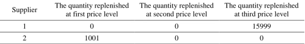
Solving the model gives results as Table 12 and 13. As is clear the first supplier supplies at the third price level and replenishes demand equal to 15999 and the second supplier supplies at the fist price level and meets demand equal to 1001.
Table 12 Each supplier’s price level and replenished quantity
The quantity replenished at third price level The quantity replenished
at second price level The quantity replenished
at first price level Supplier
15999 0
0 1
0 0
1001 2
Table 13 The optimal value of the objective functions
Returned items (Z2)
Delayed deliveries (Z3)
Cost (Z1)
Supplier
16 16
1455909000 1
15 3
1001000000 2
31 19
2456909000 Total
6. CONCLUSION AND FURTHER RESEARCH
The supplier selection problem is very important in supply management. Many various objectives and criteria should be considered. The criteria and the objectives can be stated in a crisp or fuzzy manner and can be of different importance. A company should exactly know its requirements and priorities to be able to select suitable suppliers and should have valid information about the suppliers. In this paper a comprehensive model for ranking an arbitrary number of suppliers, selecting a number of them and allocating a quota of an order to them was proposed. The two-stage logarithmic goal programming method for generating weights from interval comparison matrices (Wang et al. (2005)) was used for ranking and selecting the suppliers. A fuzzy multiobjective model was presented for quota allocation to suppliers. A case studey was given and the model was applied. The results showed that the model wotks well and could be employed in many other cases.
Further research could be improving the comprehensive model using other submodels which improve the supplier selection process or quota allocation. As an example using a model for quota allocation in case of multi-priod demand.
REFERENCES
[1] Amid A.,Ghodsypour S.H., O’Brien C.A. (2006), Fuzzy multiobjective linear model for supplier selection in a supply chain; International Journal of Production Economics 104; 394–407.
[2] Amid A., Ghodsypour S.H., O’Brien C.A. (2008), weighted additive fuzzy multiobjective model for the supplier selection problem under price breaks in a supply chain; International Journal of Production Economics 121; 323-332.
[3] Amy H.I. Lee (2008), A fuzzy supplier selection model with the consideration of benefits, opportunities, costs and risks; Expert Systems with Applications 36; 2879-2893.
[4] Arbel A. (1989), Approximate articulation of preference and priority derivation; European Journal of Operational Research; 43317–326.
[5] Arbel A. (1991), A linear programming approach for processing approximate articulation of preference, in: P. Korhonen, A. Lewandowski, J. Wallenius, (Eds.), Multiple Criteria Decision Support; Lecture Notes in Economics and Mathematical Systems 356, Springer, Berlin; 79–86.
[6] Arbel A., Vargas L.G. (1990), The analytic hierarchy process with interval judgments, in: A. Goicoechea, L. Duckstein, S. Zoints, (Eds.), 9th Internat. Conference on Multiple criteria decision making, Fairfax, Virginia, Springer, New York; 61–70.
[7] Arbel A., Vargas L.G. (1993), Preference simulation and preference programming: robustness issues in priority deviation; European Journal of Operational Research 69; 200–209.
[8] Bonder C.G. E., deGraan J.G., Lootsma. F.A. (1989), Multicriteria decision analysis with fuzzy pairwise comparisons; Fuzzy Sets and Systems 29; 133–143.
[9] Buckley J.J. (1985), Fuzzy hierarchical analysis; Fuzzy Sets and Systems 17; 233–247.
[10] Buckley J.J., Feuring T., Hayashi Y. (2001), Fuzzy hierarchical analysis revisited; European Journal of Operational Research 129; 48–64.
[11] Conde E., de la Paz Rivera Pérez M.(2010), A linear optimization problem to derive relative weights using an interval judgement matrix; European Journal of Operational Research 201(2); 537-544. [12] Csutora R., Buckley J.J. (2001), Fuzzy hierarchical analysis: the Lamda–Max method; Fuzzy Sets and
Systems 120; 181–195.
[13] Dempsey W.A. (1978), Vendor selection and buying process; Industrial Marketing Management 7; 257-267.
[14] Dickson G.W. (1966), An analysis of vendor selection systems and decisions; Journal of Purchasing 2(1); 5-17.
[15] Dopazo E., Ruiz-Tagle M.A. (2009), GP formulation for aggregating preferences with interval assessments; Lecture Notes in Economics and Mathematical Systems 618; 47-54.
[16] Dopazo E., Ruiz-Tagle M., Robles J. (2007), Preference learning from interval pairwise data. A distance-based approach; Lecture Notes in Computer Science (including subseries Lecture Notes in Artificial Intelligence and Lecture Notes in Bioinformatics) 4881 LNCS; 240-247.
[17] Geringer J.M. (1988), Joint venture partner selection: Strategies for develop countries; Westport, Quorum Books.
[18] Ghodsypour S.H, O’Brien C. (1998), A decision support system for supplier selection using an integrated analytic hierarchy process and linear programming; International Journal of Production Economics 56; 199–212.
[19] Haines L.M. (1998), A statistical approach to the analytic hierarchy process with interval judgments.(I).Distributions on feasible regions; European Journal of Operational Research 110; 112– 125.
[20] Hong G.H., Park S.C., Jang D.S., Rho H.M. (2005), An effective supplier selection method for constructing a competitive supply relationship; Expert Systems with Applications 28; 629–639.
[21] Islam R., Biswal M.P., Alam S.S. (1997), Preference programming and inconsistent interval judgments; European Journal of Operational Research 97; 53–62.
[22] Kaslingam R., Lee C. (1996), Selection of vendors – a mixed integer programming approach; Computers and Industrial Engineering 31; 347–350.
[23] Kress M. (1991), Approximate articulation of preference and priority derivation—A comment; European Journal of Operational Research 52; 382–383.
[24] Kumar M., Vrat P., Shankar R. (2004), A fuzzy goal programming approach for vendor selection problem in a supply chain; Computers and Industrial Engineering 46; 69–85.
[25] Kumar M., Vrat P., Shankar R. (2006), A fuzzy programming approach for vendor selection problem in a supply chain; International Journal of Production Economics 101; 273–285.
[26] Lee A.H.I. (2009), A fuzzy AHP evaluation model for buyer–supplier relationships with the consideration of benefits, opportunities, costs and risks; International Journal of Production Research 47; 4255-4280
[27] Leung L.C., Cao D. (2000), On consistency and ranking of alternatives in fuzzy AHP; European Journal of Operational Research 124; 102–113.
[28] Lewis J.D. (1990), Partnership for profit: structuring and managing strategic alliance; The Free Press, New York.
[29] Lin C.-W.R., Chen H.-Y. S. (2004), A fuzzy strategic alliance selection framework for supply chain partnering under limited evaluation resources; Computers in Industry 55; 159–179.
[30] Liu F.-H.F, Hai H.L. (2005), The voting analytic hierarchy process method for selecting supplier; International Journal of Production Economics 97; 308–317.
[31] Lorange P., Roos J., Bronn P.S. (1992), Building successful strategic alliances; Long Range Planning 25(6); 10–17.
[32] Mikhailov L. (2002), Fuzzy analytical approach to partnership selection in formation of virtual enterprises; Omega: International Journal of Management Science 30; 393–401.
[33] Mikhailov L. (2003), Deriving priorities from fuzzy pairwise comparison judgments; Fuzzy Sets and Systems 134; 365–385.
[34] Mikhailov L. (2004), Group prioritization in the AHP by fuzzy preference programming method; Comput. Oper. Res 31; 293–301.
[35] Moreno-Jiménez. J.M. (1993), A probabilistic study of preference structures in the analytic hierarchy process within terval judgments; Math. Comput. Modeling 17 (4/5); 73–81.
[36] Muralidharan C., Anantharaman N., Deshmukh S.G. (2002), A multi-criteria group decisionmaking model for supplier rating; Journal of Supply Chain Management 38(4); 22–33.
[37] Narasimahn R. (1983), An analytical approach to supplier selection; Journal of Purchasing and Materials Management 19(4); 27–32.
[38] Nydick R.L., Hill R.P. (1992), Using the analytic hierarchy process to structure the supplier selection procedure; Journal of Purchasing and Materials Management 25(2); 31–36.
[39] Partovi F.Y., Burton J., Banerjee A. (1989), Application of analytic hierarchy process in operations management; International Journal of Operations and Production Management 10(3); 5–19.
[40] Ravindran A.R., Bilsel R.U., Wadhwa V., Yang T. (2010), Risk adjusted multicriteria supplier selection models with applications; International Journal of Production Research 48(2); 405-424. [41] Saaty R.W. (2003), Decision making in complex environment: The analytic hierarchy process (AHP)
for decision making and the analytic network process (ANP) for decision making with dependence and feedback; Pittsburgh, Super Decisions.
[42] Saaty T.L., Vargas L.G. (1987), Uncertainty and rank order in the analytic hierarchy process; European Journal of Operational Research 32 ; 107–117.
[43] Saaty T.L. (2004), Fundamentals of the analytic network processmultiple networks with benefits, opportunities, costs and risks; Journal of Systems Science and Systems Engineering 13(3); 348–379. [44] Salo A., Hämäläinen R.P. (1992), Processing interval judgments in the analytic hierarchy process, in:
A. Goicoechea, L. Duckstein, S. Zoints, (Eds.); Proc. 9th Internat. Conference on Multiple Criteria Decision Making; Fairfax, Virginia, Springer, NewYork; 359–372.
[45] Salo A., Hämäläinen R.P. (1995), Preference programming through approximate ratio comparisons, European Journal of Operational Research 82; 458–475.
[46] Van Laarhoven P.J.M., Pedrycz W. (1983), A fuzzy extension of Saaty’s priority theory; Fuzzy Sets and Systems 11; 229–241.
[47] Wang Y.M., Chin K.S. (2006), An eigenvector method for generating normalized interval and fuzzy weights; Applied Mathematics and Computation 181(2); 1257-1275.
[48] Wang Y.M., Yang J.B.,Xu D.L. (2005), A two-stage logarithmic goal programming method for generating wehghts from interval comparison matrices; Fuzzy Sets and Systems 152; 475–498.
[49] Weber C.A., Current J.R. (1993), A multi-objective approach to vendor selection; European Journal of Operational Research 68(2); 173–184.
[50] Weber C.A., Current J.R., Benton W.C. (1991), Vendor selection criteria and methods; European Journal of Operational Research 50; 1-17.
[51] Weber C.A., Current J.R., Desai A. (1998), Non-cooperative negotiation strategies for vendor selection; European Journal of Operational Research 108; 208–223.
[52] Weber C.A, Desai A. (1996), Determination of path to vendor market efficiency using parallel coordinates representation: A negotiation tool for buyers; European Journal of Operational Research 90; 142–155.
[53] Wu D.D., Zhang Y., Wu D., Olson D.L. (2010), Fuzzy multi-objective programming for supplier selection and risk modeling: A possibility approach; European Journal of Operational Research 200(3); 774-787.
[54] Xu R. (2000), Fuzzy least-squares priority method in the analytic hierarchy process; Fuzzy Sets and Systems 112; 359–404.
[55] Xu R., Zhai X. (1996), Fuzzy logarithmic least squares ranking method in analytic hierarchy process; Fuzzy Sets and Systems 77; 175–190.
[56] Zimmermann H.J. (1978), Fuzzy programming and linear programming with several objectives functions; Fuzzy Sets and Systems 1; 45-55.

![Table 4 Interval comparison matrix for the criteria Risks Costs Opportunities Benefits [3 5] [2 3] [2 3] 1 Benefits [2 3] [1/3 ½] 1 Opportunities [3 4] 1 Costs 1 Risks](https://thumb-us.123doks.com/thumbv2/123dok_us/8371521.2223403/15.918.124.800.787.997/table-interval-comparison-criteria-opportunities-benefits-benefits-opportunities.webp)