*The author would like to acknowledge the immense collaboration and support provided by his advisor, Dr. Dan Reichart, Skynet Software Engineer Michael Maples, Lead Skynet Software Engineer Joshua Haislip, and postdoc Adam Trotter.
The Skynet Algorithm for Single-Dish Radio Mapping
Travis A. Berger
1*1 University of North Carolina at Chapel Hill Department of Physics and Astronomy
ABSTRACT
After the National Radio Astronomy Observatory’s 20-meter diameter telescope in Green Bank, West Virginia was added to the Skynet Robotic Telescope Network - which includes optical telescopes spanning four continents - a need for a radio data-processing pipeline arose. Therefore, development began to create a pipeline similar to optical Skynet’s Afterglow, and the single-dish radio mapping algorithm was born. This algorithm has a number of advantages over traditional techniques, such as basket-weaving. (1) The algorithm makes use of weighted modeling, instead of weighted averaging, to interpolate between signal measurements. This smooths the data, but without blurring it beyond instrumental resolution. Techniques that rely on weighted averaging blur point sources sometimes as much as 40%. (2) The algorithm makes use of local, instead of global, modeling to separate astronomical signal from instrumental and/or environmental signal drift along the telescope’s scans. (3) The algorithm uses a very similar, local modeling technique to separate astronomical signal from radio-frequency interference (RFI). (4) Unlike other techniques, the algorithm does not require data to be collected on a rectangular grid or regridded before processing. (5) Any pixel density may be selected for the final image. Here, the procedure is presented and evaluated using both simulated and real data. The algorithm is being integrated into the image-processing library of Skynet. Default data products will be generated on the fly, but will be customizable by the user in real time.
1. INTRODUCTION
1.1. Skynet
Founded in 2005, Skynet is a global network of fully automated, robotic, volunteer telescopes, scheduled through a common web interface. Currently, the optical telescopes range in size from 14 to 40 inches, and span four continents. It was originally created to follow-up on gamma-ray-bursts, but has since been used for studying other astronomical phenomena, a few of which include exoplanetary systems, a wide variety of variable stars, and near Earth objects. Today, Skynet’s mission is split evenly between supporting professional astronomers, students, and the public. Most users are students either those in middle school, high school, or students taking lab courses at a select number of universities throughout the country.
Figure 1: NRAO-Green Bank 20-meter diameter radio telescope. (Photo credit: NRAO)
detection, supernova remnants, quasars, and masers.
1.2. Single-Dish Mapping
While interferometry is used quite extensively throughout the field of radio astronomy, because there is only one radio telescope currently available for Skynet, it was necessary to focus on single-dish mapping. Therefore, the single-dish mapping algorithm is presented in the following pages.
1.2.1. Mapping Pattern
Many single-dish mapping algorithms (Sofue & Reich 1979, Emerson & Graeve 1988) require the signal to be sampled on a rectangular grid, where the telescope stops and integrates data at each point of this grid on the sky. However, this is an inefficient way to observe because it requires the telescope to accelerate and decelerate many times during a particular map, putting more wear-and-tear on the movement gears of the telescope. The 20-meter telescope utilizes on-the-fly (OTF) mapping, in which the signal is integrated as the telescope moves, minimizing the above concerns, as long as the integrations span no more than about 0.2 beamwidths along the telescope’s direction of motion (along the telescope’s “scan”), to avoid blurring point sources by more than 1% (Mangum, Emerson & Greisen 2007).
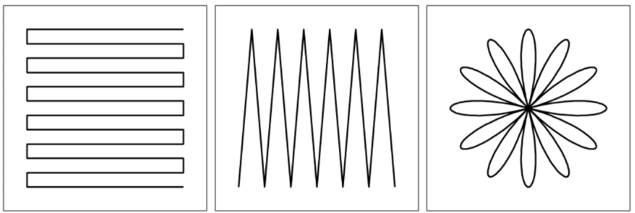
A variety of OTF mapping patterns may be employed, but only three will be discussed here (see Figure 2):
Figure 2: OTF mapping patterns. Left: Raster (horizontal). Center: Nodding. Right: Daisy.
It is important to note that as long as the gaps between any two scans are smaller than Nyquist sampling (or about 0.4 beamwidths), in theory all information between the scans can be recovered. Therefore, given the different mapping patterns available and not wanting to limit users of Skynet to any set of patterns, the algorithm must work independently of the mapping pattern.
1.2.2. Signal Averaging vs. Signal Modeling
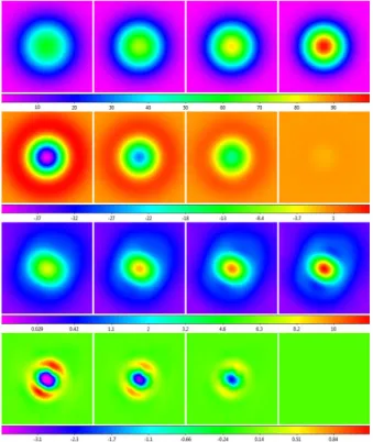
width equal to the telescopes beamwidth is used (which many seem to use), it can result in about 40% blurring and about 40% errors in the reconstructed image. To create better images, some oversample the data so that they can use a narrower kernel. The drawbacks here are two-fold: for one, oversampling takes more time and secondly, the data is still being averaged over a particular area around the desired point. For instance, Winkel, Floer, and Kraus (2012) collected about three times more data as required by Nyquist sampling, and use a ½-beamwidth kernel, yet their results still show about 12% blurring and 18% errors in the reconstructed image (see Figure 3).
Figure 3: First Row: Simulation of a point source sampled with a Gaussian beam pattern on a 1/5-beamwidth grid recovered using, from left to right: 1-beamwidth weighted averaging, 2/3-beamwidth weighted averaging, ½-beamwidth weighted averaging, and weighted modeling. Second Row: Residual error associated with each of these techniques. Third Row: Cassiopeia A observed with one of the 20-meter’s L-band linear polarization channels using a 1/5-beamwidth raster, recovered using the above techniques. One can see that weighted averaging fails to recover the telescope’s beam pattern, as well as accurately hit the true flux value of the center of the point source. Fourth Row: The difference between each of these techniques and weighted modeling. Square-root and squared scalings for the colors are used in the third and fourth rows, respectively, to emphasize fainter beam structure.
Because single-dish maps already suffer from poor resolution (when compared to interferometric maps), it would be unfortunate if the Skynet Algorithm further reduced the resolution due to processing. Therefore, the algorithm uses weighted modeling instead of weighted averaging to produce a final image. Essentially, weighted modeling fits a two-dimensional polynomial surface to the data, as long as the model is sufficiently flexible over the scale of the weighting function and the sampling is enough to over constrain this model. For instance, the weighted modeling routine is able to recover the simulated data in Figure 3 (top right corner) with <1% errors near the center of the beam pattern. It is important to note that the Skynet Algorithm uses weighted modeling as the last step of the process, not the first. Although many algorithms use weighted averaging and regridding as the first step before contaminant removal, this is a bad practice: it is always best to operate on real data for as long as possible and then approximate, interpolate, or model, not the other way around.
1.2.3. Contaminant Removal
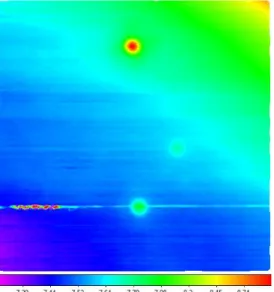
Figure 4: Raw map of Virgo A (top), 3C 270 (center right), and 3C 273 (bottom), acquired with the 20-meter in L band, using a 1/10-beamwidth horizontal raster. Left and right linear polarization channels have been independently calibrated (see §2.1) and summed, partially symmetrizing the beam pattern (Figure 3). Locally modeled surface (§1.2.1, see §2.7) has been applied for visualization only. All three signal contaminants are demonstrated: (1) en-route drift, the low-level variations along the horizontal scans, (2) an extended period of RFI, during the scan that passes through 3C 273, and (3)
elevation-dependent signal, toward the upper right,
which was only ≈11 ̊ above the horizon. Square-root
scaling is used to emphasize fainter structures.
En-route drift: Even with stable, modern receivers, the detected signal can drift in time, due to changing atmospheric emission or ground emission as the telescope moves. This results in low-level variations between scans, as can be seen above in Figure 4.
To eliminate en-route drift, others use a combination of techniques. For instance, Sofue & Reich (1979) used unsharp-masking to separate en-route drift from larger-scale structure. They then modeled the en-route drift along each scan with a second-order polynomial and used sigma-clipping to remove the contaminants. The issues with this approach include blurring the data to correct the data, using low-order polynomials to model entire scans (not a good approximation over the length of a scan), and sigma-clipping is too crude of an outlier rejection routine. Emerson & Graeve (1988) Fourier transform the data, mask it in Fourier space, and transform back. Unfortunately, this routine requires that the data consist of two orthogonal mappings, and, therefore, two rectangular grids, which is a constraint that the Skynet Algorithm must avoid. Haslam, Quigley & Salter (1970), Haslam et al. (1974), Seiber, Haslam & Salter (1979), and Haslam et al. (1981) used a technique called basket-weaving, which involves two mappings (with intersecting scans) that do not need to be orthogonal. This technique minimizes the signal differences at the intersections, but it assumes that en-route drift can be well modeled by a single low-order polynomial over the length of the scan. It also requires iteration. Winkel, Floer & Kraus (2012) introduced a routine that does not require iteration, but it does require regridding and two near-orthogonal mappings (no single maps, daisies, etc.).
RFI: Typically, RFI is localized to specific frequencies. Therefore, if spectral data is available, one can mask the particular frequencies that correspond to RFI. It is also common for RFI to be a temporal source in continuum data, characterized either by its drawn-out, en-route drift-like variation, or its short, Dirac delta function-like signature that is unlikely to occur at the same position in adjacent scans. In most of the above references, RFI was identified and then removed by hand. However, for the Skynet Algorithm, which will be utilized by a large, diverse group of people, RFI removal needs to be automatic.
Elevation-dependent signal: Atmospheric emission increases as the elevation decreases. If small- scale structures need to be preserved, it is quite easy to remove this elevation-dependent signal along with en-route drift and long-duration RFI (see §2.3). Otherwise, if large-scale structures need to be retained, then this background needs to be removed separately.
contaminants in a similar way: first, each is modeled locally (not globally) using simple parameterizations, such as first- or second-order polynomials that hold over short angular scales. To make sure that the models are as accurate as possible, the Skynet Algorithm utilizes robust Chauvenet outlier rejection to separate contaminants from the astronomical signal. Finally, the algorithm combines these locally fitted models into a global model, and then we check the procedure against simulated data.
1.2.4. Overview
In §2, we discuss the contaminant-cleaning routines and the mapping of small-scale structures. In §3 we summarize our findings and discuss future algorithm development.
2. MAPPING SMALL-SCALE STRUCTURES WITH CONTINUUM OBSERVATIONS
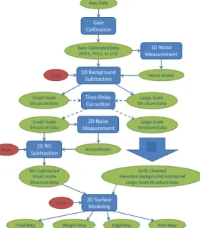
In this section, we will discuss the contaminant-cleaning routines and the mapping of small-scale structures (and all of the required routines to do so as accurately as possible). First, gain-calibration and “robust” Chauvenet outlier rejection (and its uses) will be introduced. Then, we measure the noise in each scan, using an iterative point-to-point variation routine. With these newly-determined noise measurements, each scan can then be separated into large-scale contaminants and the astronomical signal using an iterative background-modeling routine. The algorithm then subtracts the modeled background from the real data. Next, cross-correlation is used in-between consecutive scans to measure and correct for any time delay between the coordinate and integrated signal measurements. After cross-correlation, we utilize robust Chauvenet rejection, but this time to measure the noise level across scans. This new across-scan noise measurement, along with the previous one within the scans, allows the algorithm to separate astronomical small-scale structure from short-duration RFI. Finally, after RFI removal is finished, the algorithm employs a weighted modeling interpolation routine to produce an image of contaminant-cleaned data, without blurring it beyond instrumental limitations (§1.2.2).
Figure 5: Flowchart of the Skynet Algorithm for contaminant-cleaning and mapping small-scale structures. Blue are the component algorithms. Green are the inputs to and outputs of these component algorithms, consisting of data, corresponding noise models, and ultimately maps. Red are user-selected scales, for separating wanted and unwanted structures, and for modeling the final surface.
2.1. Gain Calibration and “Robust” Chauvenet Outlier Rejection
As with any other precision instrument, the 20-meter telescope needs to be gain-calibrated correctly before its data products can provide physically viable astronomical information. After significant testing, it was found that 20-meter’s
gain varies negligibly over the course of an observation. Therefore, we perform calibration at the beginning and at the end of observations instead of in-between scans. The Skynet Algorithm allows users to choose either the initial calibration (Δ1), final calibration (Δ2), or a linear
However, this technique is sensitive to possible outliers that may occur during the on and off periods of calibration, so the algorithm uses a variation of Chauvenet outlier rejection that we call “robust” Chauvenet rejection to reject these outliers. Essentially, Chauvenet rejection is an improvement on sigma clipping, as sigma clipping does not account for the size of a set of data. For instance, in a data set of 100 points, 2-sigma variations are expected, but 4-sigma variations would be extreme. However, in a data set of 10000 points, 3-sigma variations would be expected, but 5-sigma variations would not. The criterion for Chauvenet rejection is as follows:
𝑁𝑃 > 𝑧 <0.5, (1)
where N is the total number of points and P(> |z|) is the cumulative probability that a particular measurement is more than z standard deviations from the mean of a Gaussian distribution. However, the mean and the standard deviation are usually unknown, so we must measure them from the data. Nevertheless, both the mean and the standard deviation are very sensitive to the outliers within the data that the algorithm is trying to reject.
Therefore, “robust” Chauvenet rejection is used, which determines the 50th-percentile value (the median) and the 68.3-percentile deviation. These quantities approximate the mean and the standard deviation, respectively, but both are significantly less sensitive to outliers. We apply the routine iteratively to the calibration data, rejecting one point at a time to ensure stability (see Figure 6).
Figure 6: 40-foot gain calibration data, with the noise diode first on (high points) and then off (low points). Circled points have been robust Chauvenet rejected, including data taken during the transitions and RFI- contaminated data (discrepant points within each set of high or low points).
The algorithm calibrates each polarization channel separately, but then processes three maps, one for each polarization channel and the other for the combined, averaged, flux-calibrated two channels. We will employ Robust Chauvenet rejection in the many sections ahead.
2.2. 1D Noise Measurement
Figure 7: Point-to-point noise measurement technique. Top: Applied to gain-calibrated 20-meter data. The circled point at the top has been robust Chauvenet rejected. Bottom: A plot of the residuals (after subtraction). The median and 68.3-percentile values are calculated from the non-rejected points.
To make sure that this technique gives accurate values, we tested it on a data set of Gaussian random noise with a known mean of zero and a standard deviation of one. We found that the point-to-point technique overestimates the noise’s true standard deviation by about 22.9%. Therefore, each scan’s point-to-point noise measurement is corrected accordingly by multiplying by 0.814 (to correct for the overestimation). Now that the algorithm has determined the point-to-point noise measurements of every scan, it can combine them into a single model that accounts for changes in the noise level with time by fitting a quadratic polynomial to the noise as a function of scan number. Again, we use robust Chauvenet rejection to reject overly discrepant point-to-point noise scans (see Figure 8).
Figure 8: Corrected 1D noise measurements vs. scan number for a particular 20-meter observation. As can be seen by the circled points, only two noise measurements were rejected, although this is unusual because all of the discrepant intra-scan measurements have been rejected. Here, the noise level increases by about 20% from the beginning to the end of the observation.
2.3. 1D Background Subtraction
Now that the algorithm has a noise level for each scan at its disposal, it now has a criterion for which it can model backgrounds throughout each scan. With the 1D background subtraction routine, the goal is to
separate all large-scale contaminants (en-route drift, long-duration RFI, elevation-dependent signal) from the small-scale astronomical point sources and short-duration RFI. Since long-duration RFI and en-route drift are 1D structures that vary along the scans, the algorithm begins by modeling and subtracting structures larger than the user-defined scale along the scans only (1D background subtraction).
before the upgrade empirically by two different criteria. The first required that the background scale at multiple parallactic angles did not affect the peak value of a point source, and the second required that the entire structure of the beam pattern (including faint outskirts) was visible. Therefore, the minimum for the first criterion was determined to be 6.5 beamwidths, and the second 8 beamwidths.
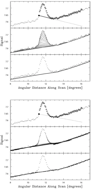
Using this scale, the basic approach to 1D background subtraction is to draw a line from each point to another point within one scale length, such that all other points (within this scale length) are above the line. We then repeat this for each point, but in the backward direction, and the minimum of all the linear individual models is a non-linear background model. Although this does work pretty well in modeling the shape of the background, it underestimates the true background behavior (see Figure 9).
Figure 9: Top: A forward-directed local background model, anchored to a point in a scan going across 3C 270 in Figure 4. Circled points are within one background scale length, but are above the model. Middle: Forward- and backward-directed local background models, each corresponding to a point in the scan.
Bottom: The global background model, constructed from all of the local background models. Notice how it rides under the background and not through it, as it should.
In addition to riding under the true background structure, this algorithm is also very sensitive to negative noise fluctuations. Therefore, using a similar but superior routine, the algorithm gives better results (see Figure 10).
Figure 10: Top: A forward-directed local background model, anchored to the same point as in Figure 9. This time, however, all of the circled points have been iteratively rejected (as they are above the calculated noise level) using robust Chauvenet rejection. Middle: Final local background models originally (but no longer) anchored to every point in the scan. Bottom:
The global background model, which has been constructed from the linear final local background models (solid curve), and from the quadratic local background models (dashed curve).
specific set of points within the desired, calculated noise measurement. Next, the algorithm rejects the anchor point and refits to the non-rejected points, resulting in a lower standard deviation. To raise the deviation back up to the calculated value determined in §2.2, the routine iteratively adds the least-outlying rejected points to the left and right of the non-rejected points until the standard deviation value is consistent with the noise measurement. This gives a final local background model for each of the points in the scan (Figure 10, middle panel). Consequently, the model does not underestimate nor overestimate the background behavior. To construct the final, global background model illustrated in the bottom panel of Figure 10, the algorithm again uses robust Chauvenet rejection to reject outliers and determine the median value for each point in these background models. However, based upon the nature of these models, and the fact that points toward the center of fitted data are better constrained than those on the edges, each of the points must be weighted by the number of non-rejected points contributing to its local background model and by its position in its local background model:
𝑤!" = !!
!!!!"!!!!
!
!
!! !!"!!!!
!
!, (2)
where wij is the weight of the jth point of the ith local background model, xij is the angular
distance of this point along the scan, Ni is the number of non-rejected points to which the ith local
background model was fitted, µi is the average angular distance of these points along the scan, σi
is the standard deviation of these values, τi is the values’ kurtosis:
𝜏! =
!!"!!!!
!
!!!
!
!/!
, (3)
and δ is zero for linear local background models and one for quadratic local background models. For the rest of this paper, quadratic local background models are used because of their increased flexibility over linear background models, and their robustness (insensitivity to wild variations and above noise-level errors).
2.3.1. Simulation: Gaussian Random Noise
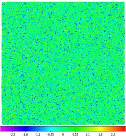
In the next few sections, we will test the background subtraction algorithm by applying it to simulated data of increasing complexity. The first test is on a grid of Gaussian random noise (Figure 11).
Figure 11: 20-meter 1/10th-beamwidth horizontal raster
replaced with Gaussian noise. This noise has a mean of zero and a standard deviation equal to one. The locally modeled surface (see §2.7) has been used for visualization only.
the data is simply flat noise. Therefore, how close the residuals are to zero is an important metric of the quality of the background subtraction routine.
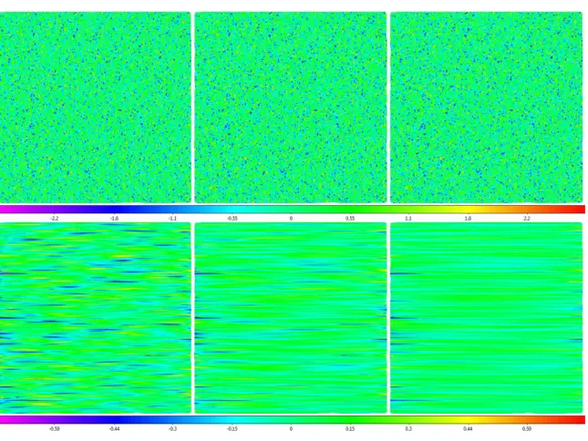
Figure 12: Top row: Data from Figure 11 background-subtracted with 6-, 12-, and 24-beamwidth scales, moving from left to right. The map is 24-24-beamwidths across. Bottom row:
Data from Figure 11 minus the top row (at each of the different scales, respectively). As can be seen from the colors, background-subtracted data is biased neither high nor low. The noise levels of the data sets in the top row, from left to right, are ~97.8%, ~98.7%, and ~99.1% compared to the noise level of Figure 11, while the noise level of the residuals are only ~19.7%, ~15.1%, and ~12.1% respectively. Locally modeled surfaces have been applied for visualization only.
Overall, the background subtraction algorithm works as expected in subtracting flat data, and smaller angular scales result in higher RMS noise in the residuals, while larger background subtraction scales have lower RMS noise. The reason for this is the difference in quality of each of the background subtractions (which is directly related to the number of points available to fit to within each scale).
2.3.2. Simulation: Small-Scale Structures
background-subtracting Figure 13 at each of the scales.
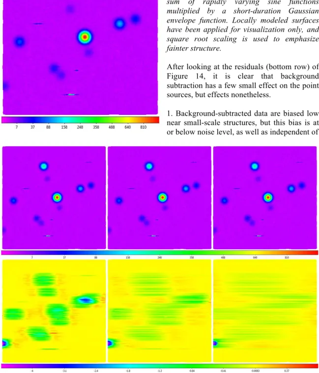
Figure 13: Simulated data from Figure 11 to which we have added Gaussian point sources and short-duration RFI. To create the short duration RFI, we use the absolute value of a sum of rapidly varying sine functions multiplied by a short-duration Gaussian envelope function. Locally modeled surfaces have been applied for visualization only, and square root scaling is used to emphasize fainter structure.
After looking at the residuals (bottom row) of Figure 14, it is clear that background subtraction has a few small effect on the point sources, but effects nonetheless.
1. Background-subtracted data are biased low near small-scale structures, but this bias is at or below noise level, as well as independent of
residuals are biased negative, and that each of the different scales result in residuals of ~1/2 – 1, ~1/4 – 1/2, and ~1/8 – 1/4 of the noise level from left to right. Larger residuals are possible when small-scale structures blend with large-scale structures, and even larger residuals will occur at the end of scans. Locally modeled surfaces have been applied for visualization only, and square root and squared scalings are used in the top and bottom rows, respectively, to show fainter structures.
the brightness of the small-scale structure. For example, we see that the 1000 signal/noise point source in the middle gives about the same residuals as the other ~10 signal/noise sources across the image. The bias level is greatest in the center of these regions, and is only dependent upon the noise level (directly proportional) and the background subtraction scale (inversely proportional), not the brightness of the source. Although this is an introduction of systematic error, the error that it does introduce is so low that it can be ignored.
2. Unfortunately, the bias can be somewhat larger when small-scale structures are blended together (look at Figure 14, bottom row on the left at the area of blue on the right side of the image). The reason for this is that the two point sources, when blended together, become a larger structure that may exceed the user’s background subtraction scale. For instance, the 6-beamwidth background subtraction scale is smaller than the blended structure, so it gives residuals about 2.5 times the noise level, but the 12- and 24-beamwidth scales show typical, sub-noise level residuals. However, we will eliminate background subtraction bias in §3.
3. The bias can be significantly larger when small-scale structures fall at the end of a scan. The reason for this is that our models run out of data to fit to near the end of a scan (the brightness of the source in the top row at the bottom left of each of the images of Figure 14 is about 40% smaller than it should be). Unfortunately, not too much can be done about this right now, although this issue should be largely resolved in §3.
2.3.3. Simulation: 1D Large-Scale Structures
Next, simulated long-duration RFI and en-route drift are added to our simulation data from §2.3.2. We follow the same procedure in this section, where background subtraction is used on 6-, 12-, and 24-beamwidth scales.
The residuals are presented in the bottom row of Figure 16, but here we have only subtracted off the residuals from the bottom rows of Figures 12 and 14 to emphasize the residuals from the large-scale 1D structures only.
Figure 16: Top row: Data from Figure 15 after background subtraction with 6-, 12-, and 24-beamwidth scales. Bottom row: Data from the top row minus the data from Figure 14 (residuals) and the Gaussian residuals from the bottom row of Figure 12. En-route drift and long-duration RFI are not eliminated, but are significantly reduced, especially for the shorter background subtraction scales (6-beamwidth). These long-duration contaminants are again reduced significantly when we remove RFI in §2.6. Locally modeled surfaces have been applied for visualization purposes only, and square root and hyperbolic-arcsine scalings are used in the top and bottom rows, respectively, to emphasize faint structures.
Figure 17:Top: Factor by which background subtraction reduces en-route drift (red), long-duration RFI (green), large-scale astronomical signal (blue), and elevation-dependent signal (black). Bottom: Fraction of the noise level to which the above are reduced.
2.3.4. Simulation: 2D Large-Scale Structures
Next, we add simulated large-scale 2D structures to the data in Figure 15 (see Figure 18). We then follow a similar procedure as we did in the previous sections, first using 6-, 12-, and 24-beamwidth baselines for background subtraction (and the producing the resultant images), and then determining the residuals afterwards.
Figure 19: Top row: Data from Figure 18 after background subtraction with 6-, 12-, and 24-beamwidth scales (from left to right). Bottom row: Data from the top row minus the data from Figure 16 (residuals), Figure 14 (residuals), and the Gaussian residuals from the bottom row of Figure 12. The elevation-dependent signal is effectively eliminated, while the large-scale astronomical signal is not completely eliminated, but is significantly reduced, especially for the shorter background subtraction subtraction scales (6-beamwidth). The large-scale contaminants are again reduced, but only marginally, when we remove RFI in §2.6. Locally modeled surfaces have been applied for visualization purposes only, and square root and squared scalings are used in the top and bottom rows, respectively, to emphasize faint structures.
Figure 19 illustrates these products, but it is important to note that, to emphasize the residuals of these 2D large-scale structures, we have subtracted out the residuals from the bottom rows of Figures 12, 14, and 16. As mentioned in Figure 19’s caption, the algorithm is effective at reducing/eliminating these large-scale contaminants, especially on smaller beamwidth scales of background subtraction. Quantitatively, we find that large-scale astronomical signal and elevation-dependent signal are reduced by factors of about 15 and 190, to about 3 times and 17% of the noise-level, respectively, when using a background subtraction scale of 24-beamwidths (the size of the map). For a subtraction scale of 12-beamwidths, we reduce the large-scale astronomical signal and elevation-dependent signal by factors of about 510 and 710, to about 9% and 5% of the noise level, respectively. We reduce these structures by even greater factors at smaller scales (see Figure 17). After RFI removal (see §2.6), these numbers are reduced even further, albeit minimally.
If one looks very hard at the 6-beamwidth scale residual map, one can see that additional noise and sub-noise level residuals remain near small-scale structures. These residuals can be either negative or positive, depending upon the nature of the background around the small-scale structures, but, as in §2.3.2, the residuals are not very significant and we should almost completely remove them after we model large-scale structures in §3. As before, there are also relatively large residuals near the end of scans, but again we will eliminate these after RFI subtraction in §2.6 and large-scale structure modeling in §3.
Figure 20: Left: Figure 4 after background subtracting with an 8-beamwidth scale. Right:
Figure 4 after background subtracting with a 24-beamwidth scale. The locally modeled surface has been applied for visualization only, and square root scaling is used to emphasize fainter structures.
After having applied this algorithm to almost every case of simulated data, we can now move onto real data. First, we apply it to the 20-meter L-band raster in Figure 4 (see Figure 20). As can be seen from both the left and the right images, we successfully eliminated the elevation-dependent signal. In addition, much of the 1D and 2D large-scale structures are significantly reduced. However, streaks remain from the background subtraction, although RFI subtraction will remove these artifacts (§2.6).
Figure 21: Top row: Time-corrected (see §2.4) raw maps of Andromeda (left and middle), acquired with the 40-foot telescope in L-band, using a maximum slew speed nodding pattern (Figure 2, middle). The difference of the left and right panels is displayed in the rightmost column. Instrumental signal drift dominates each map.
Bottom row: Data from the top rows background subtracted using a 5-beamwidth scale. Despite the overwhelming instrumental signal in the top maps, the source is extracted (and the maps look similar) after background subtraction! Locally modeled surfaces have been applied for visualization only.
In Figure 21, we have applied the algorithm to 40-foot maps that utilize the nodding pattern in Figure 2. Clearly, the 40-foot’s stability is inferior to the 20-meter’s, although after subtracting the top left and middle panels of Figure 21, the result is noise level fluctuations.
Figure 22: Left: Raw map of 3C 84 in X band using the 20-meter’s 20-petal daisy pattern. Right: Left, after background subtraction with an 8.6-beamwidth scale (the map is 8.6-beamwidths across). A locally modeled surface has been applied for visualization purposes only, and hyperbolic arcsine scaling is used to emphasize fainter structure.
map of 3C 84 to demonstrate this algorithm’s application to non-rectangular mapping patterns. We treat each slew of the telescope across the diameter of the observing region as a separate scan for background subtraction purposes.
2.4. Time-Delay Correction (Optional)
Both the 20-meter and 40-foot telescopes perform on-the-fly integration of signal as they create these 2D maps. Unfortunately, the integrated signal values do not always match up with the correct right ascension (RA) and declination (DEC) because of a time delay in between read outs of the RA and DEC and the integrated flux value. This lack of synchronization is always present in 40-foot maps because of a RC filter with a time-constant of 0.1 seconds. This essentially delays the flux measurements, resulting in maps that look like the top left corner of Figure 23. The 20-meter, on the other hand, integrates the signal over a user-defined time, and the position is recorded at the midpoint of the integration time, effectively eliminating any time-delay issues in maps.
Figure 23: Top row: 40-foot L band map of the sun after background subtraction. The left image is done without time-delay correction, while the right image is after time-delay correction. If one looks closely at the left image, one can see zig-zags near the edge of the red portion of the source, indicating the time-delay problem. The six spokes illustrate the diffraction pattern of the 40-foot telescope, and the center is saturated. Bottom row: 20-meter background-subtracted map of Cassiopeia A in L band, where the 20-meter’s signal and position computers’ clocks are not synchronized in the left image. In the right image, we utilized our time-delay correction routine. Locally modeled surfaces have been applied for visualization purposes only, and hyperbolic arcsine scaling is used to emphasize fainter structures.
median value must be divided by the median slew speed of the telescope (for rasters or noddings), which is measured from the data (robustly, of course). We then take this time and shift each signal measurement accordingly by interpolating the telescope’s position that time ago. For daisies, the telescope’s slew speed changes constantly and it reaches its max in the center of the desired source. Therefore, we use this maximum slew speed instead of the median of the other maps because of source domination.
In terms of when this correction procedure should be done, it is best to proceed with time-delay correction after background subtraction, as cross-correlation works best when it is dominated by sources, not the noisy background present in pre-background-subtracted data.
2.5. 2D Noise Measurement
The key to RFI removal in the next section is the 2D noise determination on the newly background-subtracted data. We approach this issue similarly to how we dealt with the 1D noise measurement. Except, this time, the noise is measured across the scans instead of through them.
For each point, we draw a line between the most-similar point in the previous scan and the most similar point in the next scan. We then measure the deviation of the center point from this line (see Figure 24). We use robust Chauvenet rejection to determine the median and 68.3-percentile deviation for each scan of these deviations. Outliers are typically caused by RFI and signal variations around bright sources, but Chauvenet rejection, as in §2.1, rejects these. The final noise measurement (what we call the scan-to-scan noise measurement) is the sum in quadrature of the final median and the final 68.3-percentile deviation.
Figure 24: Scan-to-scan noise measurement technique applied to rasters (top left), noddings (top right), daisies (bottom left). Residuals are measured as in the bottom right panel, and the median and 68.3-percentile deviation values are determined from the non-rejected residuals from each scan.
2.6. 2D RFI Subtraction
Before going completely into our 2D RFI subtraction routine, we will note that this code remains in development as of late. Originally, we utilized a 1D RFI subtraction routine that fit a one-parameter, squared-cosine model to each scan, similar to how we used a three-parameter quadratic to model the background throughout a scan. However, this 1D RFI’s goal was to eliminate any structures smaller than a particular scale. Therefore, point sources that are blurred to the telescope’s diffraction limit could be retained, and any short-duration, temporal RFI would be eliminated. To do this, we fit a 1D squared cosine function with a particular FWHM (specified by the user) to the data within each scan. If the cosine function could fit “up into” a source, it was retained. Otherwise, anything that the squared cosine could not fit into would be eliminated, as the squared cosine function would only fit to the points corresponding to the bottom of the temporal spike. Therefore, any points above the squared cosine function through iteration would be dropped down to noise-level fluctuations (see Figure 26).
Our new algorithm, however, makes use of a 2D squared cosine function. Like the 1D RFI subtraction routine, the 2D algorithm also has many similarities to the background subtraction routine, but there are a few key differences:
1. 2D RFI subtraction separates sub-beamwidth structures from larger structures, instead of hyper-beamwidth structures from smaller structures.
2. Instead of using a three-parameter quadratic local model, we utilize a one-parameter squared cosine local model:
𝑧 Δθ =𝑓𝑐𝑜𝑠! !"#
!!!"# 𝑖𝑓 Δθ<θ!"#. (4)
This is set to zero if Δθ > θRFI, where Δθ is the angular distance and θRFI is the user-defined RFI
subtraction scale, and f, the free parameter, normalizes the function. The arguments within the cosine function are chosen so that when θRFI is about 1-beamwidth, it mimics a
background-subtracted point source with shorter wings (see Figure 25). In addition, the beauty of this specific squared cosine function allows us to choose the θRFI to correspond to a number just shy of the
telescope’s true FWHM of its beam pattern so we can separate very small-scale structures from those that correspond to important point sources that we want to preserve.
Figure 25: Local squared cosine model (solid line) with θRFI = 1, Airy function (dashed line), and
Gaussian function (dotted line), each with FWHM = 1-beamwidth.
To go into more detail, the iterative process consists of centering on every point in a scan, and then fitting the squared cosine function to all points within range (Δθ < θRFI). The standard deviation of these points
non-rejected points is consistent with the noise model (see Figure 26).
Figure 26: First: 1D cross-section, along a scan, of a 2D local model, centered on an arbitrary point from the left panel of Figure 3, near Virgo A. We have contaminated the scan with three instances of simulated RFI. Circled points have been iteratively rejected as being above the modeled noise level. Second: 1D cross-sections of every 2D local model that intersects this scan. Boxes correspond to single-point 1D cross-sections. All instances of simulated RFI have been rejected as too narrow, either along this scan or across adjacent scans, compared to the RFI-subtraction scale (in this case θRFI = 1 beamwidth). Third: Global model, constructed from the local models. Fourth: Original, uncontaminated data and resulting, nearly identical, global model.
After the iterations finish, a single local model remains for only the non-rejected points. We then repeat this process for every point (as the center) in the observation, resulting in a collection of local models.
3. As in §2.3, we construct the global model from the local models by taking the median of the local models at each point and iteratively rejecting outliers through robust Chauvenet rejection. Again, we must weight each of the models for each of the points based upon its accuracy (dependent upon its position in the local model):
𝑤!"=!!(!!!!!"), (5)
where wij is the weight of the jth point in the ith local model, Δθij is the angular distance of this
point from the model’s center, and Ni is the number of non-rejected points utilized by the ith local
model. However, unlike in §2.3, we do not subtract the global model from the data. The global model, in this routine, is the RFI subtracted result. This model is a smoother version of the original data, but it does not result in any additional blurring.
In theory, we should be able to choose the RFI subtraction scale, θRFI, up to the true FWHM of
the telescope’s beam pattern. However, as with most routines in practice, choosing a FWHM within that vicinity may result in partial subtraction of point sources. The reason for this is that beam patterns of telescopes are not necessarily perfect (they may be peaked more in one direction than another, or even asymmetric. Therefore, it is necessary for us to choose a smaller RFI subtraction scale. The recommended values for θRFI are yet to be determined (a discussion of
future analysis/routines will be given in §3).
Figure 27: Left: See Figure 18 for caption. Middle: The left panel after 6-beamwidth background subtraction. Right: The left panel after 6-beamwidth scale background subtraction and 0.5-beamwidth scale 1D RFI subtraction. Locally modeled surface has been applied for visualization purposes only, and hyperbolic arcsine, square root, and square root scalings were used (from left to right).
Qualitatively, it is clear that we have significantly decontaminated the image on the left after sending it through background subtraction and 1D RFI subtraction (result: right image). We will perform quantitative analysis as soon as the 2D RFI subtraction algorithm is perfected.
2.7. 2D Surface Modeling
In this section, we present our 2D surface-modeling algorithm which regrids the data into an image. As was discussed back in §1, our algorithm’s approach is unique among other the algorithms described in other papers, as it uses weighted modeling instead of averaging and can be used after the data has been cleaned of contaminants. It is also important to stress that modeling is superior to averaging because it does not blur the original data. Moreover, our routine can be applied after any particular step, if visualization is wanted. As the reader has seen, there have been many examples (see many of the figures) throughout this paper illustrating the results of the surface-modeling algorithm.
Additionally, this approach allows us to arbitrarily choose the pixel density of the final image, unlike other routines that require regridding data to perform their contaminant cleaning routines. We have set a default pixel scale of 1/20th of a beamwidth, but the user can change this scale. For each pixel, we fit a flexible, third-order, 2D polynomial function to all data within 1-beamwidth of the center pixel. In addition, we weight the points higher the closer they are to the center pixel. Our modeling routine utilizes:
𝑧 Δ𝑥,Δ𝑦 = !!!! !!!!!!𝑎!"(Δ𝑥)!(Δ𝑦)!, (6)
where z is the locally modeled signal, Δx and Δy are the angular distances from the center pixel along each direction, and aij are the polynomial coefficients. We determine z for every pixel in the
image.
of the modeled surface. We use the following weighting function:
𝑤 Δθ =𝑐𝑜𝑠! !"#
! 𝑖𝑓 Δθ<1 𝑏𝑒𝑎𝑚𝑤𝑖𝑑𝑡ℎ,𝑤ℎ𝑒𝑟𝑒 α=−
!"# (!) !"# (!"# !!!! ) (6)
and where θw is the user-defined FWHM of the weighting function, and w = 0 if Δθ >
1-beamwidth.
Figure 28: Weighting function with FWHM
θw = 1/3- (solid), 2/3- (dashed), and 1-
(dotted) beamwidths.
From the above equations, it can be shown rather easily that a choice of a smaller θw
results in a larger α, therefore favoring the data that is closer to the central pixel. However, smaller θw values reduce the
precision of the fit, as the local modeled surface has less data points to which to fit. It is important to note that choosing θw values
below about 1/3-beamwidth provides no additional benefit, as RFI subtraction should eliminate information smaller than 1/3-beamwidths.
Expectedly, there is a “sweet spot” for this
θw; making the angular radius of weighting too small results in fits that are under constrained and
likely discrepant. Therefore, it is necessary to define θw more robustly:
θ!=max !! 𝑏𝑒𝑎𝑚𝑤𝑖𝑑𝑡ℎ𝑠,!!×θ!"# , (7)
where θgap is a measure of the largest distance between any two consecutive scans in an entire
observation. This works very well with rasters and noddings, but daisies are a unique challenge, due to their odd shape and the unclear division of scans. Noddings are slightly more complicated than rasters because of the large differences between consecutive scans (at turn-around points the scans are very close together), but it again comes down to the largest angular gap between consecutive sweeps in any area of the map. For daisies, we again adapt a largest gap model to account for the lack of points a single local model may have, but this time there are three gap factors, each dependent upon the radius away from the center of the pattern. These three gap factors are the inter-, and intra-petal gaps, as well as the robust Chauvenet-rejected median gap along the scans. These gaps cannot exceed ¾-beamwidths or else the model will be under constrained and it will likely arrive at a wrong modeled value for that particular point in the grid.
The Skynet algorithm will also be able to append multiple observations/maps, but that section of the code remains in development with preliminary tests looking promising.
2.7.1. Applications to Asymmetric Structures
terms for z (see page 21), the locally-modeled signal. See Figure 29 for an example.
Figure 29: 3-minute 20-meter X-band raster of Centaurus A, background-subtracted, time-delay corrected, and RFI-removed. The radio jet is marginally resolved and oriented correctly with respect to the galaxy (right). Optical picture of NGC 5128 (left) taken with Skynet’s PROMPT-2 telescope at Cerro-Tololo Inter-American Observatory, courtesy of the Star Shadows Remote Observatory astrophotography group.
2.7.2. Default Data Products
After completing each 20-meter or 40-foot mapping, Skynet automatically produces the following data products for the left, right, or combined polarizations (or any combination of the three):
Raw maps: Maps produced by our surface-modeling algorithm immediately after reading the signal, so the user can visualize the data before processing. A θw scale of 4/3*θgap is used to better
visualize sub-beamwidth contaminants.
Contaminant-cleaned maps: Maps produced by our surface-modeling algorithm after data processing, which includes gain-calibration, background subtraction, time-delay correction, RFI subtraction, and finally surface modeling, using the user-recommended scales or our recommended values for each step.
Path maps: A grid of the same size as the contaminant-cleaned maps and raw maps is created, but the path maps instead use values of one and zero to distinguish the path that the telescope “draws” on the sky. A one (1) or negative one (-1) is given to points at particular angular coordinates at which signal integration occurs (alternating each scan), and all others are given zeros. Path maps are useful for determining whether the telescope had any issues in mapping the sky or whether the encoders for the RA or DEC malfunctioned.
Scale maps: These maps visualize the weighting scale used for each surface-modeled point. Rasters are usually very simple (a single value across the entire map), but daisies’ and noddings’ scale maps are much more complicated and vary over the grid. Scale maps are important for photometry (see §2.8), as only regions of images with θw ≤ 1/3-beamwidths should be trusted.
stack/average images, as weights need to be appropriately determined when averaging. We use weight maps later in our photometry routine and in the production of the edge maps.
Edge maps: These maps measure how far any pixel in an image is from the edge of the data, and as one approaches the edge of an image, there may not be enough data to adequately constrain the surface-modeling polynomial. Therefore, when generating the final images, we remove the pixels that are too far from the rest of the data using the edge map. We generate these maps by calculating a “center-of-mass” for each collection of data points to which Equation 6 was fitted. The criterion for which we remove pixels from the final contaminant-cleaned maps is still being tested, although the most recent value was found to be about 0.1 weighting scales, where greater values exclude the pixel from the final image. However, this threshold will be configurable so the user can see more or less of the image if need be.
2.8. Aperture Photometry
Because this algorithm produces a contaminant-cleaned, accurately modeled surface spanning a grid of pixels, one can perform operations on it, much as one would on a reduced optical image. Therefore, the algorithm can utilize a simple aperture photometry routine to measure the brightness of astronomical sources. The only requirement for aperture photometry is that the locally modeled surface was produced with a weighting scale less than ~1/3-beamwidths.
We perform photometry by slapping a circular aperture and a concentric annulus around a source of interest. We do this by determining the center-of-mass of the pixel values within the aperture and iterating as necessary. The photometry routine then sums these values, subtracting a constant, near-background value calculated from the robust Chauvenet rejection-determined weighted median value of the annulus. This routine is still in development, pending further testing.
3. FUTURE WORK AND CONCLUSIONS
Ultimately, our algorithm succeeds in removing contaminants from radio maps, regardless of the mapping pattern used. The algorithm requires no further work in noise determination, background subtraction, or weighted modeling mapping. However, the 2D RFI removal routines still require further work. In addition, we will use spectral data to facilitate the removal of RFI of specific frequencies. We must also implement code to clean and map large-scale structures separately from the small-scale structure code already present. Finally, once development of the algorithm is complete, we will implement the code into Skynet. Once implemented, we will generate default data products that are customizable by the user in real time. Ultimately, Radio Skynet will provide a means to make the invisible sky visible to a diverse group of people for years to come.
REFERENCES
Emerson, D. T. & Graeve, R. 1988, Astronomy & Astrophysics
Haslam, C. G. T., Klein, U., Salter, C. J., et al. 1981, Astronomy & Astrophysics
Haslam, C. G. T., Quigley, M. J. S., & Salter, C. J. 1970, Monthly Notice of the Royal Astronomical Society
Haslam, C. G. T., Wilson, W. E., Graham, D. A., & Hunt, G. C. 1974, Astronomy & Astrophysics Supplement
Mangum, J. G., Emerson, D. T., & Greisen, E. W. 2007, Astronomy & Astrophysics Sieber, W., Haslam, C. G. T., & Salter, C. J. 1979, Astronomy & Astrophysics Sofue, Y. & Reich, W. 1979, Astronomy & Astrophysics Supplement