ORIGINAL ARTICLE
The dynamic relationship between oil prices and exchange rates
Hamid SakakiCentral Connecticut State University ,Department of Finance, , 1615 Stanley St, New Britain, CT 06053, USA
Abstract: Using daily data of oil prices and exchange rates of 14 countries for the period January 1999 to November 2014, this study examines the dynamic correlation between oil prices and exchange rates using the DCC-GARCH model. The results show the significantly negative correlation between oil prices and exchange rates over the period. These results imply that the increase of oil price coincides with US dollar depreciation and vice versa. This correlation strengthens in a negative direction during periods of financial crisis, while it shifts to an upward trend after the financial crisis period.
Keywords: Oil price; exchange rate; dynamic correlation
1. Introduction
Crude oil is an influential factor in contemporary economic and political movements (Huang et al., 1996). Eleven recessions took place in the US between World War II and 2014 and in ten of them, oil prices increased just before the shocks. Over the last decade, the US dollar lost its value against major currencies such as the Japanese Yen, and the Australian and Canadian dollar. By July 2008, oil prices had risen to more than $140 per barrel and the US dollar depreciated against other major traded currencies. Understanding the relationship between exchange rate and oil price is an interesting topic to study because appreciation or depreciation of the US dollar is the subject of debate among scholars. The goal of this paper is to examine the dynamic relationship between oil prices and exchange rates with DCC-GARCH model by using daily data from 01/01/1999 to 01/11/2014 of 14 countries which include exporting, importing and neither exporting nor importing.
Overall, the results show the significantly negative dynamic correlation between oil prices and exchanges rate over the period. These results imply that the increase of oil price coincides with US dollar depreciation and vice versa. This correlation strengthens in a negative direction during the financial crisis period, while it shifts to an upward trend post-crisis.
I organize the remainder of this paper in this order. Section 2 reviews related literature on the relationship between oil prices and exchange rates. Section 3 describes data and sample, research design, and methodology is discussed in Section4. I describe results and summarize model outputs in Section 5, and conclude the paper in Section 6.
2. Literature review
There are many studies on the relationship between oil prices and exchange rates. One of the pioneering works is Hamilton (1983). He establishes the link between oil price increases and the US business cycle. Following Hamilton (1983), Golub (1983) and Krugman (1983) show that when oil price increases, oil exporting countries may experience Copyright © 2017 Hamid Sakaki
doi: 10.18686/fm.v2i2.909
This is an open-access article distributed under the terms of the Creative Commons Attribution Unported License
(http://creativecommons.org/licenses/by-nc/4.0/), which permits unrestricted use, distribution, and reproduction in any medium, provided the original work is properly cited.
appreciation and oil importing countries may experience depreciation. Also, Blomberg and Harris (1995) examine the impact of exchange rate on oil price by the law of one price. They show that US dollar depreciation can increase the purchasing power of foreigners and this leads to oil demand going up. As a result, the oil price moves up.
On the one hand, Amano and van Norden (1998) examine the link between the real effective value of the US dollar and the price of oil by cointegration and error correction models using monthly data from 1972 to 1993. They find that an increase in oil price leads to the appreciation of the US dollar in the long-run. Also, Benassy-Quere et al. (2007) using monthly data from 1974 to 2004 show the same results by cointegration and causality tests. In addition, Chen and Chen (2007), using monthly data of G7 countries by panel cointegration find the existence of a significant long-term equilibrium relationship where a rise in oil price depreciates the local currency against the US dollar. Moreover, Ghosh (2011) using the GRACH and EGARCH models for India from July 2007 to November 2008 reports evidence of US dollar appreciation when the oil price increases.
On the other hand, Narayan et al. (2008) using daily data from November 2000 to September 2006 examine the relationship between oil price and the Fijian dollar against the US dollar by using GARCH and EGARCH models. They find that a rise in oil prices leads to appreciation of the Fijian dollar against the US dollar. Akram (2009) applya structural VAR model using quarterly data from 1990 to 2007 and find the depreciation of the US dollar leads to higher oil prices and that US dollar shocks significantly account for oil price fluctuations. Also, Wu et al. (2012) examine the economic value of comovement between oil price and US dollar using weekly data from 1990 to 2009 by Copula-GARCH models and show that the dependence structure between oil and exchange rate returns becomes negative and decrease continuously after 2003. Recently, Turhan et al. (2013) by using VAR and daily data of emerging countries conclude that an increase in oil prices appreciates local currencies against the US dollar. Also, Turhanet al. (2014) apply the cDCC model to analyze the dynamic correlation of G20 countries by using daily data from 2000 to 2013. They show that for each pair of oil price-exchange rate, evidence confirms a strengthening negative correlation in the last decade.
Although the link between oil price and exchange rate has been widely investigated in literature, the results are mixed. The empirical evidence generally suggests that exchange rate and oil prices are co-integrated (where causality may run in both directions). Some studies show that an increase in oil price leads to US dollar appreciation (e.g. Amano and van Norden, 1998; Benassy-Quereet al., 2007; Ghosh, 2011), while others find that an increase in oil price causes US dollar depreciation (e.g. Narayanet al., 2008; Akram, 2009; Wuet al., 2012; Turhanet al., 2013; Turhanet al., 2014) against other currencies. The fact that the rise in oil price is associated with depreciation or appreciation of the US dollar may be due to the level of oil dependence of different countries. Lizardo and Mollick (2010) add the oil price to the monetary model of exchange rate in the long-run and show that the US dollar against oil exporter currencies (Canada, Mexico, and Russia) depreciates in response to oil price increases. In contrast, oil price increases lead to the appreciation of the US dollar against oil importer currencies, such as Japan. They also show that the US dollar depreciates against the currencies of countries that are neither oil exporters nor oil importers such as, the UK and the European Union.
3. Data
All data series in this study are daily retrieved from the Federal Reserve Economic Data for the period January 1, 1999, to November 1, 2014. There are two motivations for choosing this period. First, the start date of this period is after the Asian financial crisis in 1997. The oil price fell dramatically in 1998 and recovered after that. Second, this study period includes the recent financial crisis iof 2008.
I use daily data in this study because not only exchange rates but also oil prices change every day in response to financial forces and news. This means high frequency data captures the impact of oil price on exchange rate return more precisely. Many related studies use daily data (e.g. Narayanet al., 2008; Zhanget al., 2008 and Turhanet al., 2014). I consider oil price per barrel, West Texas Intermediate (WTI) as the oil price in this study. The reasons I use the prices of
0.8 1.2 1.6 2.0 2.4
2000 2002 2004 2006 2008 2010 2012 2014
AUD 1.0 1.5 2.0 2.5 3.0 3.5 4.0
2000 2002 2004 2006 2008 2010 2012 2014
BRL 0.8 1.0 1.2 1.4 1.6 1.8
2000 2002 2004 2006 2008 2010 2012 2014
CAD 0.6 0.8 1.0 1.2 1.4 1.6 1.8 2.0
2000 2002 2004 2006 2008 2010 2012 2014
CHF 4 5 6 7 8 9 10
2000 2002 2004 2006 2008 2010 2012 2014
DKK .45 .50 .55 .60 .65 .70 .75
2000 2002 2004 2006 2008 2010 2012 2014
GBP 30 40 50 60 70
2000 2002 2004 2006 2008 2010 2012 2014
INR 60 80 100 120 140
2000 2002 2004 2006 2008 2010 2012 2014
JPY 8 10 12 14 16
2000 2002 2004 2006 2008 2010 2012 2014
MXN 4 5 6 7 8 9 10
2000 2002 2004 2006 2008 2010 2012 2014
NOK 20 25 30 35 40 45
2000 2002 2004 2006 2008 2010 2012 2014
RUB 1.0 1.2 1.4 1.6 1.8 2.0
2000 2002 2004 2006 2008 2010 2012 2014
SGD 28 30 32 34 36
2000 2002 2004 2006 2008 2010 2012 2014
TWD 0 40 80 120 160
2000 2002 2004 2006 2008 2010 2012 2014
WTI 4 6 8 10 12 14
2000 2002 2004 2006 2008 2010 2012 2014
ZAR
-8 -4 0 4 8 12
2000 2002 2004 2006 2008 2010 2012 2014
RET_AUD -12 -8 -4 0 4 8 12
2000 2002 2004 2006 2008 2010 2012 2014
RET_BRL -6 -4 -2 0 2 4 6
2000 2002 2004 2006 2008 2010 2012 2014
RET_CAD -8 -4 0 4 8 12
2000 2002 2004 2006 2008 2010 2012 2014
RET_CHF -6 -4 -2 0 2 4
2000 2002 2004 2006 2008 2010 2012 2014
RET_DKK -6 -4 -2 0 2 4
2000 2002 2004 2006 2008 2010 2012 2014
RET_GBP -4 -2 0 2 4
2000 2002 2004 2006 2008 2010 2012 2014
RET_INR -6 -4 -2 0 2 4
2000 2002 2004 2006 2008 2010 2012 2014
RET_JPY -8 -4 0 4 8
2000 2002 2004 2006 2008 2010 2012 2014
RET_MXN -8 -4 0 4 8
2000 2002 2004 2006 2008 2010 2012 2014
RET_NOK -8 -4 0 4 8
2000 2002 2004 2006 2008 2010 2012 2014
RET_RUB -3 -2 -1 0 1 2 3
2000 2002 2004 2006 2008 2010 2012 2014
RET_SGD -3 -2 -1 0 1 2 3
2000 2002 2004 2006 2008 2010 2012 2014
RET_TWD -20 -10 0 10 20
2000 2002 2004 2006 2008 2010 2012 2014
RET_WTI -10 -5 0 5 10
2000 2002 2004 2006 2008 2010 2012 2014
RET_ZAR
-.6 -.4 -.2 .0 .2
2000 2002 2004 2006 2008 2010 2012 2014
CORR_AUD_WTI -.6 -.4 -.2 .0 .2
2000 2002 2004 2006 2008 2010 2012 2014
CORR_BRL_WTI -.6 -.4 -.2 .0 .2
2000 2002 2004 2006 2008 2010 2012 2014
CORR_CAD_WTI -.4 -.3 -.2 -.1 .0 .1 .2
2000 2002 2004 2006 2008 2010 2012 2014
CORR_CHF_WTI -.6 -.4 -.2 .0 .2 .4
2000 2002 2004 2006 2008 2010 2012 2014
CORR_DKK_WTI -.5 -.4 -.3 -.2 -.1 .0 .1
2000 2002 2004 2006 2008 2010 2012 2014
CORR_GBP_WTI -.6 -.4 -.2 .0 .2
2000 2002 2004 2006 2008 2010 2012 2014
CORR_INR_WTI -.6 -.4 -.2 .0 .2
2000 2002 2004 2006 2008 2010 2012 2014
CORR_MXN_WTI -.6 -.4 -.2 .0 .2
2000 2002 2004 2006 2008 2010 2012 2014
CORR_NOK_WTI -.8 -.6 -.4 -.2 .0 .2
2000 2002 2004 2006 2008 2010 2012 2014
CORR_RUB_WTI -.6 -.4 -.2 .0 .2
2000 2002 2004 2006 2008 2010 2012 2014
CORR_SGD_WTI -.6 -.4 -.2 .0 .2 .4
2000 2002 2004 2006 2008 2010 2012 2014
CORR_ZAR_WTI
Figure 3. Mean level shifts in the dynamic correlations estimated by DCC between WTI (in us dollar) and exchange rates (local currencies against USD) of 14 countries. Vertical lines indicate the shifts in correlation level
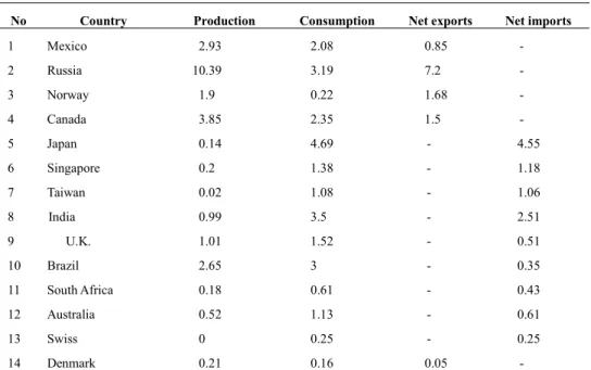
the West Texas Intermediate (WTI) are two-fold. First, they are the most widely used indices in North America. Second, when firms use hedging instruments, the vast majority use futures, forwards and other derivative contracts based on the WTI. Also, the data includes bilateral exchange rates of 14 countries. These 14 countries include exporting; importing and neither oil exporters nor oil importers because oil price could affect the exchange rates of these countries differently. For this purpose, I collect the daily average of oil production and consumption of each country in 2012 and calculate the net import or net export of each country. Table 1 presents the list of countries and their daily average of oil production and consumption in 2012. Based on Table 1 and literature, the currencies are classified into three groups: net exporting (Mexico, Russia, Norway and Canada), net importing (Japan, Singapore, Taiwan, India) and neither oil exporters nor oil importers (Brazil, South Africa, Australia, Swiss, U.K and Denmark). Killian et al. (2009) consider Mexico, Norway, and Russia as the oil exporters and the US, Japan, and the Euro area as oil importers. Also, Lizardo and Mollick (2010) classify countries into three groups. In their study, oil exporters are Canada, Mexico, Norway, and Russia; Japan is an oil importers. They classify the UK and the European Union as neither net exporters nor significant importers. Recently, Beckmann and Czudaj (2013) consider Brazil, Canada, Mexico, Norway, and Russia as the major oil-exporting countries as well as the Euroarea, India, Japan, South Africa, South Korea, Sweden, and the UK as oil-importing countries.
Table 1- List of countries
No Country Production Consumption Net exports Net imports
1 Mexico 2.93 2.08 0.85
-2 Russia 10.39 3.19 7.2
-3 Norway 1.9 0.22 1.68
-4 Canada 3.85 2.35 1.5
-5 Japan 0.14 4.69 - 4.55
6 Singapore 0.2 1.38 - 1.18
7 Taiwan 0.02 1.08 - 1.06
8 India 0.99 3.5 - 2.51
9 U.K. 1.01 1.52 - 0.51
10 Brazil 2.65 3 - 0.35
11 South Africa 0.18 0.61 - 0.43
12 Australia 0.52 1.13 - 0.61
13 Swiss 0 0.25 - 0.25
14 Denmark 0.21 0.16 0.05
-Notes: – Oil production and consumption of 14 countries in 2012 (million barrels per day)
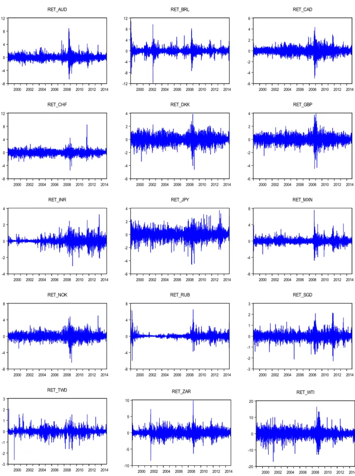
Figure 1 and 2 present the graphs for the variables in level and return, respectively. Based on Figure 1, it is apparent that the US dollar depreciates against major currencies (AUD, CAD, CHF, and JPY) over the last decade except from 2008 to 2009. During the financial crisis period, almost all local currencies depreciate against the US dollar. On the other hand, the levels of the WTI oil index show a slight downturn after the technology bubble, but a rapid rise and fall during the financial crisis in 2008. Such fluctuation in the oil price leads us to question its impact on different exchange rates. In addition, Figure 2 presents the daily volatilities of exchange rate returns and oil prices. Based on Figure 2, all currencies have the most fluctuations during financial crisis periods. Also, it is evident that Russia and India have managed float currencies.
4. Methodology
The model used in this study is Dynamic Conditional Correlation (DCC) – GARCH, as processed by Engle (2002). Eq. (1) presents the mean equation of DCC-GARCH:
REY_EXt=a0+b1RET_EXt-1+b2REI_WTIt-1+εt (1)
where, RET_EXt is the daily return of local currencies against US dollars, RET_WTIt−1 is WTI daily returns and εt is an error term with a conditional variance matrix:
Ht=DtRtDt (2)
where, Dt is the n×n diagonal matrix of time-varying standard deviation from univariate GARCH models with
hii,t on the ith diagonal, i=1 and 2; Rt is the n×n time-varying correlation matrix.
The DCC-GARCH model, proposed by Engle (2002), involves a two-stage estimation of the conditional covariance matrix. The first stage requires the selection of appropriate univariate GARCH models, in order to obtain the standard deviations, hii,t. In the second stage, currency return residuals adjust by their estimated standard deviations from the first stage, uit = εit / hii,t , then uit is used to estimate the parameters of conditional correlation. Eq. (3) represents the correlation in DCC:
Qt=(1-a-b)Q+αut−1ut−1' +βQt−1 (3)
where, Qt = (qij,t) is the n×n time varying covariance matrix of ut, Q = E (utut') is the n×n unconditional variance matrix of ut , and a and b are nonnegative scalar parameters satisfying (a+b)<1. Then it is necessary to re-escalate the matrix Qt in order to guarantee that all the elements in the diagonal be equal to one. As a result, we obtain a proper correlation matrix Rt
-Rt=(diag (Qt))−1 2Qt(diag (Qt))−1 2 (4)
where, (diag (Qt))−1 2 = diag (1 q11,t ,…,1 qnn,t).
Eq. (3) is a correlation matrix with ones on the diagonal and off-diagonal elements less than one in absolute value, as long as Qt is positive definite. Eq. (5) is show typical element of Rt:
Pij,t= qqij,t
ii,t∗qjj,t ( i, j = 1, 2 and i≠ j) (5)
For avoiding potential serial correlation, I apply a white noise test. LBSQ (5) and (20) stand for the Ljung-Box statistic of 5th and 20th order, respectively applied to the squared standardized residuals. If the P-value is significant, the errors are not white noise and there is a serial correlation between error terms.
5. Results
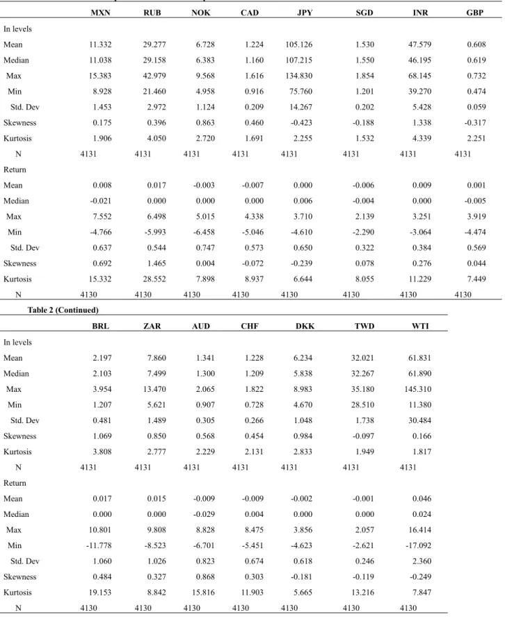
Table 2 reports the descriptive statistics of exchange rate and WTI for the period study: Jan 1, 1999, to Nov 1, 2014. The average daily return for NOK, CAD, SGD, AUD, CHF, DKK and TWD is negative, while it is positive for the rest of the sample over the period except JPY which is zero. Also, the average daily return for oil price is 0.046% over the study period.
Table 3 presents the DCC-GARCH results for 14 countries. The time-varying correlation coefficient of standardized residuals between exchange rate and WTI is significantly negative for all except JPY and TWD. This result suggests that when the oil price increases the US dollar depreciates against local currencies and vice versa. Indeed, this link doesn’t depend on the dependency of countries to oil and this is same for all countries. Also, Table3 reports the results of theLjung-Box test of order 5 and 25. The result suggests that all errors are white noise.
Table 2 - Descriptive statistics of the sample
MXN RUB NOK CAD JPY SGD INR GBP
In levels
Mean 11.332 29.277 6.728 1.224 105.126 1.530 47.579 0.608
Median 11.038 29.158 6.383 1.160 107.215 1.550 46.195 0.619
Max 15.383 42.979 9.568 1.616 134.830 1.854 68.145 0.732
Min 8.928 21.460 4.958 0.916 75.760 1.201 39.270 0.474
Std. Dev 1.453 2.972 1.124 0.209 14.267 0.202 5.428 0.059
Skewness 0.175 0.396 0.863 0.460 -0.423 -0.188 1.338 -0.317
Kurtosis 1.906 4.050 2.720 1.691 2.255 1.532 4.339 2.251
N 4131 4131 4131 4131 4131 4131 4131 4131
Return
Mean 0.008 0.017 -0.003 -0.007 0.000 -0.006 0.009 0.001
Median -0.021 0.000 0.000 0.000 0.006 -0.004 0.000 -0.005
Max 7.552 6.498 5.015 4.338 3.710 2.139 3.251 3.919
Min -4.766 -5.993 -6.458 -5.046 -4.610 -2.290 -3.064 -4.474
Std. Dev 0.637 0.544 0.747 0.573 0.650 0.322 0.384 0.569
Skewness 0.692 1.465 0.004 -0.072 -0.239 0.078 0.276 0.044
Kurtosis 15.332 28.552 7.898 8.937 6.644 8.055 11.229 7.449
N 4130 4130 4130 4130 4130 4130 4130 4130
Table 2 (Continued)
BRL ZAR AUD CHF DKK TWD WTI
In levels
Mean 2.197 7.860 1.341 1.228 6.234 32.021 61.831
Median 2.103 7.499 1.300 1.209 5.838 32.267 61.890
Max 3.954 13.470 2.065 1.822 8.983 35.180 145.310
Min 1.207 5.621 0.907 0.728 4.670 28.510 11.380
Std. Dev 0.481 1.489 0.305 0.266 1.048 1.738 30.484
Skewness 1.069 0.850 0.568 0.454 0.984 -0.097 0.166
Kurtosis 3.808 2.777 2.229 2.131 2.833 1.949 1.817
N 4131 4131 4131 4131 4131 4131 4131
Return
Mean 0.017 0.015 -0.009 -0.009 -0.002 -0.001 0.046
Median 0.000 0.000 -0.029 0.004 0.000 0.000 0.024
Max 10.801 9.808 8.828 8.475 3.856 2.057 16.414
Min -11.778 -8.523 -6.701 -5.451 -4.623 -2.621 -17.092
Std. Dev 1.060 1.026 0.823 0.674 0.618 0.246 2.360
Skewness 0.484 0.327 0.868 0.303 -0.181 -0.119 -0.249
Kurtosis 19.153 8.842 15.816 11.903 5.665 13.216 7.847
N 4130 4130 4130 4130 4130 4130 4130
Notes: Daily data from Jan 1 1999 to Nov 1 2014. Table 3 - DCC_GARCH results
Mean equation parameters
MXN RUB NOK CAD JPY SGD INR
RET_EX 0.0188 0.0511*** -0.00952 -0.0134 -0.0170 -0.00944 0.0229
(0.016) (0.017) (0.016) (0.016) (0.016) (0.016) (0.017)
RET_WTI -0.0103** -0.00342*** -0.00189 -0.0134*** -0.00645 -0.00414** 0.00175*
(0.004) (0.001) (0.004) (0.003) (0.004) (0.001) (0.001)
Variance equation parameters
α 0.0537*** 0.107*** 0.0330*** 0.0428*** 0.0385*** 0.0526*** 0.0943***
(0.005) (0.010) (0.003) (0.004) (0.005) (0.005) (0.008)
β 0.939*** 0.904*** 0.962*** 0.954*** 0.952*** 0.935*** 0.911***
(0.005) (0.008) (0.004) (0.004) (0.006) (0.007) (0.006)
Additional estimation output and diagnostics
Correlation -0.274*** -0.228*** -0.254*** -0.271** -0.00868 -0.229** -0.110*
(0.075) (0.085) (0.056) (0.112) (0.028) (0.092) (0.061)
lambda1 0.0147*** 0.0190*** 0.0145*** 0.0135*** 0.0159*** 0.00954*** 0.0101***
(0.002) (0.003) (0.002) (0.002) (0.004) (0.002) (0.002)
lambda2 0.982*** 0.977*** 0.980*** 0.984*** 0.964*** 0.989*** 0.986***
(0.003) (0.004) (0.002) (0.002) (0.012) (0.003) (0.002)
LBSQ (5) 5.333 10.273 3.991 0.917 2.214 8.156 4.6725
[0.37] [0.06] [0.55] [0.96] [0.81] [0.14] [0.74]
LBSQ(20) 12.914 5.956 9.773 12.421 14.430 29.403 6.9883
[0.88] [0.65] [0.97] [0.90] [0.80] [0.18] [0.35]
N 4,129 4,129 4,129 4,129 4,129 4,129 4,129
Table 3 (Continued) Mean equation parameters
GBP BRL ZAR AUD CHF DKK TWD
RET_EX 0.0118 0.0190 0.0258 0.0188 -0.0108 0.00353 0.0355*
(0.016) (0.016) (0.016) (0.016) (0.016) (0.016) (0.019)
RET_WTI -0.00428 -0.00446 0.000506 -0.0103** 0.000296 -0.00647 -0.00710***
(0.003) (0.004) (0.005) (0.004) (0.004) (0.004) (0.001)
Variance equation parameters
α 0.0399*** 0.117*** 0.0743*** 0.0537*** 0.038*** 0.0300*** 0.210***
(0.005) (0.008) (0.006) (0.005) (0.004) (0.003) (0.018)
β 0.954*** 0.877*** 0.923*** 0.939*** 0.958*** 0.968*** 0.780***
(0.005) (0.008) (0.006) (0.005) (0.004) (0.003) (0.016)
Additional estimation output and diagnostics
Correlation -0.220*** -0.286* -0.215*** -0.274*** -0.14*** -0.204*** -0.109
lambda1 0.00747*** 0.0091*** 0.0181*** 0.0147*** 0.012*** 0.0147*** 0.00401***
(0.002) (0.002) (0.003) (0.002) (0.002) (0.002) (0.001)
lambda2 0.990*** 0.989*** 0.977*** 0.982*** 0.978*** 0.979*** 0.995***
(0.003) (0.002) (0.003) (0.003) (0.004) (0.003) (0.001)
LBSQ (5) 1.927 8.966 2.480 3.817 1.639 0.944 4.9055
[0.85] [0.11] [0.77] [0.57] [0.89] [0.96] [0.17]
LBSQ(20) 21.218 24.157 20.296 17.144 21.817 8.102 5.5937
[0.38] [0.23] [0.43] [0.64] [0.35] [0.99] [0.87]
N 4,129 4,129 4,129 4,129 4,129 4,129 4,129
Notes: Daily data from Jan 1 1999 to Nov 1 2014. Each currency pair (RET_EX) consists of exchange rates quoted as one US dollar expressed in units of local currency. RET_WTI is the return of oil price in US dollar. Standard errors in parentheses. P values in squared brackets. ***, ** and * denote significance at the 1, 5 and 10% level respectively. LBSQ (5) and (20) stand for the Ljung-Box statistic of 5th and 20th order, respectively applied to the squared standardized residuals. For each country the mean equation is RET_EXt = a0 + b1RET_EXt−1 +b2 RET_WTIt−1+ εt and the variance equation is hii,t = ci + αi εi,t−12 + βi
hii,t−1 , i=1, 2.
Table 4 - shift dates of the dynamic correlation levels estimated by DCC between WTI and exchange rates of 14 countries.
MXN_WTI SGD_WTI AUD_WTI
Date ρ Date ρ Date ρ
7/30/20
08 down 7/16/2008 down 8/5/2008 down
10/6/20
11 up 7/9/2012 up 7/3/2012 up
RUB_WTI INR_WTI GBP_WTI
Date ρ Date ρ Date ρ
3/18/20
08 down 3/5/2008 down 1/23/2008 down
8/7/201
2 up 8/3/2012 up 10/5/2012 up
NOK_WTI CHF_WTI BRL_WTI
Date ρ Date ρ Date ρ
3/19/20
08 down - - 7/30/2008 down
5/6/201
1 up 7/3/2012 up 9/18/2012 up
CAD_WTI DKK_WTI ZAR_WTI
Date ρ Date ρ Date ρ
7/18/20
08 down 3/18/2008 down 8/5/2008 down
10/7/20
11 up 7/3/2012 up 8/6/2012 up
Regarding thevariance equation, α and β are significant for all currencies and the sum of α and β is close to one for all, which indicates that volatility shocks are persistent.
Figure 3 depicts mean level shifts in the dynamic correlations estimated by DCC between WTI (in US dollar) and exchange rates (local currencies against US dollar) of 14 countries. The exact shift dates are given in Table 4.The correlation shifts in two specific periods. In particular, the first shift for all (except CHF) is during 2008. The first shift starts with GBP on 1/23/2008 and not so later these shifts are followed by other currencies. This shift intensified the negative correlation. The second shift occurs post-crisis period for all. This shift starts with NOK on 5/06/2011. After this date shifts for the rest of the sample follow in late 2011 and 2012. In contrast to the first shift, the second shift has an upward trend. The dynamic correlation between WTI and exchange rate experience surprising changes so that it
reaches zero or even becomes positive for the RUB, NOK,CAD, CHF, DKK AUD and ZAR for a very short period. This second shift implies that the correlation between WTI and exchange rate is becomes weaker post the crisis period. Turhan et al. (2014) predict this shift in their study. They discuss that based on the speech of Bernake on May 22, 2013 the excess liquidity is going to run out and access to liquidity isn’t as easy as before. Consequently, investors move their capital away from riskier investments to the safest possible investment financial assets. As a result, the dynamic correlation changes to the pre-crisis level as it is based on Figure 3.
6. Conclusion
This paper examines the dynamic correlation estimated by DCC between WTI (in US dollar) and exchange rates (local currencies against USD) of 14 countries. Overall, the evidence shows that the dynamic correlation is negative and significant for all except JPY and TWD. These results imply that oil price increases coincidewith US dollar depreciation and vice versa. This study finds two significant shifts between correlations over the period. The first shift occurs during financial crisis and the negative correlation is augmented. It makes sense because during a financial crisis period most countries use oil as a financial asset. So, the usage of oil as a financial instrument makes it sensitive to other asset prices. The second change happens after the financial crisis. The postcrisis period leads to the weakening of this correlation and this correlation back to pre-2008 status. The shortage of liquidity accounts for this shift as investors are more willing to invest in the safest financial assets, such as governmental bonds, and this dynamic correlation becomes weaker.
References
1. Huang, R.D., Masulis, R.W., Stoll, H.R., 1996. Energy shocks and financial markets. Journal of Futures Market 16, 1–27. 2. Lizardo, Radhamés A., and André V. Mollick. "Oil price fluctuations and US dollar exchange rates." Energy Economics 32.2
(2010): 399-408.
3. Golub, S., 1983. Oil prices and exchange rates. Economics Journal 93, 576–593.
4. Hamilton, J.D., 1983. Oil and the macroeconomy since World War II. Journal of Political Economy 99, 228–248.
5. Krugman, P., 1983. Oil and the dollar. In: Bhandari, J.S., Putnam, B.H. (Eds.), Economic Interdependence and Flexible Exchange Rates. Cambridge University Press, Cambridge.
6. Blomberg, S.B., Harris, E.S., 1995. The commodity-consumer price connection: fact or fable? Federal Reserve Board of New YorkEconomic Policy Review 1, 21–38.
7. Amano, R.A., Van Norden, S., 1998. Oil prices and the rise and fall of the US real exchange rate. Journal of International Moneyand Finance 17, 299–316.
8. Benassy-Quere, A., Mignon, V., Penot, A., 2007. China and the relationship between the oil price and the dollar. Energy Policy35, 5795–5805.
9. Chen, S.S., Chen, H.C., 2007. Oil prices and real exchange rates. Energy Economics 29, 390–404.
10. Ghosh, S., 2011. Examining crude oil price-exchange rate nexus for India during the period of extreme oil price volatility. Applied Energy 88, 1886–1889.
11. Akram, Q.F., 2009. Commodity prices, interest rates and the dollar. Energy Economics 31, 838–851.
12. Narayan, P.K., Narayan, S., Prasad, A., 2008. Understanding the oil price-exchange rate nexus for the Fiji islands. Energy Economics30, 2686–2696.
13. Wu, C.C., Chung, H., Chang, Y.H., 2012. The economic value of co-movement between oil price and exchange rate using copulabased GARCH models. Energy Economics 34, 270–282.
14. Turhan, M.I., Hacihasanoglu, E., Soytas, U., 2013. Oil prices and emerging market exchange rates. Emerging Markets Finance andTrade 49, 21–36.
15. Turhan, M. I., Sensoy, A., & Hacihasanoglu, E. (2014). A comparative analysis of the dynamic relationship between oil prices and exchange rates. Journal of International Financial Markets, Institutions and Money, 32, 397-414.
16. Kilian, Lutz, and Cheolbeom Park, 2009, The impact of oil price shocks on the US stock market, International Economic Review 50, 1267-1287.
17. Engle, R.F., 2002. Dynamic conditional correlation: a simple class of multivariate generalized autoregressive conditional het-eroskedasticity models. Journal of Business & Economic Statistics 20, 339–350.
18. G7 is a group consisting of Canada, France, Germany, Italy, Japan, UK and USA. G7 representing more than 64% of the net global wealth ($263 trillion) according to the Credit Suisse Global Wealth Report October 2014