A R
EDUCTION
A
PPROACH TO
C
ONSTRAINED
R
EINFORCEMENT
L
EARNING
Anonymous authors
Paper under double-blind review
ABSTRACT
Many applications of reinforcement learning (RL) optimize a long-term reward subject to risk, safety, budget, diversity or other constraints. Though constrained RL problem has been studied to incorporate various constraints, existing methods either tie to specific families of RL algorithms or require storing infinitely many individual policies found by an RL oracle to approach a feasible solution. In this paper, we present a novel reduction approach for constrained RL problem that ensures convergence when using any off-the-shelf RL algorithm to construct an RL oracle yet requires storing at most constantly many policies. The key idea is to reduce the constrained RL problem to a distance minimization problem, and a novel variant of Frank-Wolfe algorithm is proposed for this task. Throughout the learning process, our method maintains at most constantly many individual poli-cies, where the constant is shown to be worst-case optimal to ensure convergence of any RL oracle. Our method comes with rigorous convergence and complex-ity analysis, and does not introduce any extra hyper-parameter. Experiments on a grid-world navigation task demonstrate the efficiency of our method.
1
INTRODUCTION
Contemporary approaches in reinforcement learning (RL) largely focus on optimizing the behavior of an agent against a single reward function. RL algorithms like value function methods (Zou et al., 2019; Zheng et al., 2018) or policy optimization methods (Chen et al., 2019; Zhao et al., 2017) are widely used in real-world tasks. This can be sufficient for simple tasks. However, for complicated applications, designing a reward function that implicitly defines the desired behavior can be challenging. For instance, applications concerning risk (Geibel & Wysotzki, 2005; Chow & Ghavamzadeh, 2014; Chow et al., 2017), safety (Chow et al., 2018) or budget (Boutilier & Lu, 2016; Xiao et al., 2019) are naturally modelled by augmenting the RL problem with orthant constraints. Exploration suggestions, such as to visit all states as evenly as possible, can be modelled by using a vector to measure the behavior of the agent, and to find a policy whose measurement vector lies in a convex set (Miryoosefi et al., 2019).
To solve RL problem under constraints, existing methods either ensure convergence only on a spe-cific family of RL algorithms, or treat the underlying RL algorithms as a black box oracle to find in-dividual policy, and look for mixed policy that randomizes among these inin-dividual policies. Though the second group of methods has the advantage of working with arbitrary RL algorithms that best suit the underlying problem, existing methods have practically infeasible memory requirement. To get an-approximate solution, they require storingO(1/)individual policies, and an exact solu-tion requires storing infinitely many policies. This limits the prevalence of such methods, especially when the individual policy uses deep neural networks.
In this paper, we propose a novel reduction approach for the general convex constrained RL (C2RL) problem. Our approach has the advantage of the second group of methods, yet requires storing at most constantly many policies. For a vector-valued Markov Decision Process (MDP) and any given target convex set, our method finds a mixed policy whose measurement vector lies in the target convex set, using any off-the-shelf RL algorithm that optimizes a scalar reward as aRL oracle. To do so, the C2RL problem is reduced to a distance minimization problem between a polytope and a convex set, and a novel variant of Frank-Wolfe type algorithm is proposed to solve this distance minimization problem. To find an-approximate solution in anm-dimensional vector-valued MDP,
Table 1: Comparison with previous approaches. To find an-approximate solution, time complexity under orthant or convex constraints is compared using the numbers of RL oracle calls. The memory requirement is measured by the number of individual policies stored for an-approximate solution.
Method Orthant constraint Convex constraint Converge for any RL algo. No extra hyper-parameter Memory requirement
Tessler et al. (2018) To a fixed point 7 7 7 1
Le et al. (2019) O(1/) 7 3 7 O(1/)
Miryoosefi et al. (2019) O(1/) O(1/) 3 7 O(1/)
C2RL (this paper) O(1/) O(1/) 3 3 ≤m+ 1
our method only stores at mostm+ 1policies, which improves from infinitely manyO(1/)(Le et al., 2019; Miryoosefi et al., 2019) to a constant. We also show thism+ 1constant is worst-case optimal to ensure convergence of RL algorithms using deterministic policies. Moreover, our method introduces no extra hyper-parameter, which is favorable for practical usage. A preliminary experimental comparison demonstrates the performance of the proposed method and the sparsity of the policy found.
2
RELATED
WORK
For high dimensional constrained RL, one line of approaches incorporates the constraint as a penalty signal into the reward function, and makes updates in a multiple time-scale scheme (Tessler et al., 2018; Chow & Ghavamzadeh, 2014). When used with policy gradient or actor-critic algorithms (Sutton & Barto, 2018), this penalty signal guides the policy to converge to a constraint satisfying one (Paternain et al., 2019; Chow et al., 2017). However, the convergence guarantee requires the RL algorithm can find a single policy that satisfies the constraint, hence ruling out methods that search for deterministic policies, such as Deep Q-Networks (DQN) (Mnih et al., 2013), Deep Deterministic Policy Gradient (DDPG) (Lillicrap et al., 2015) and their variants (Van Hasselt et al., 2015; Wang et al., 2016; Fujimoto et al., 2018; Barth-Maron et al., 2018).
Another line of approaches uses a game-theoretic framework, and does not tie to specific families of RL algorithm. The constrained problem is relaxed to a zero-sum game, whose equilibrium is solved by online learning (Agarwal et al., 2018). The game is played repeatedly, each time any RL algorithm can be used to find abest responsepolicy to play against a no-regret online learner. Themixed policythat uniformly distributed among all played policies can be shown to converge to an optimal policy of the constrained problem (Freund & Schapire, 1999; Abernethy et al., 2011). Taking this approach, Le et al. (2019) uses Lagrangian relaxation to solve the orthant constraint case, and Miryoosefi et al. (2019) uses conic duality to solve the convex constraint case. However, since the convergence is established by the no-regret property, the policy found by these methods requires randomization among policies found during the learning process, which limits their prevalence. Different from the game-theoretic approaches, we reduce the C2RL to a distance minimization prob-lem and propose a novel variant of Frank-Wolfe (FW) algorithm to solve it. Our result builds on recent finding that the standard FW algorithm emerges as computing the equilibrium of a special convex-convave zero sum game (Abernethy & Wang, 2017). This connects our approach with pre-vious approaches from game-theoretic framework (Agarwal et al., 2018; Le et al., 2019; Miryoosefi et al., 2019). The main advantage of our reduction approach is that the convergence of FW algorithm does not rely on the no-regret property of an online learner. Hence there is no need to introduce extra hyper-parameters, such as learning rate of the online learner, and intuitively, we can eliminate un-necessary policies to achieve better sparsity. To do so, we extend Wolfe’s method for minimum norm point problem (Wolfe, 1976) to solve our distance minimization problem. Throughout the learning process, we maintain an active policy set, and constantly eliminate policies whose measurement vector are affinely dependent of others. Unlike norm function in Wolfe’s method, our objective function is not strongly convex. Hence we cannot achieve the linear convergence of Wolfe’s method as shown in Lacoste-Julien & Jaggi (2015). Instead, we analyze the complexity of our method based on techniques from Chakrabarty et al. (2014). A theoretical comparison between our method and various approaches in constrained RL is provided in Table 1.
3
PRELIMINARIES
Avector-valued Markov decision processcan be identified by a tuple{S,A, β, P,c}, whereSis a set of states,Ais the set of actions andβis the initial state distribution. At the start of each episode, an initial states0 is drawn following the distributionβ. Then, at each stept = 0,1, . . ., the agent observes a statest ∈ Sand makes a decision to take an actionat. Afteratis chosen, at the next
observation the state evolves to statest+1 ∈ Swith probabilityP(st+1|st, at). However, instead
of a scalar reward, in our setting, the agent receives anm-dimensional vectorct ∈ Rmthat may
implicitly contain measurements of reward, risk or violation of other constraints. The episode ends after a certain number of steps, called the horizon, or when a terminate state is reached.
Actions are typically selected according to a policyπ, whereπ(s)is a distribution over actions for anys ∈ S. Policies that take a single action for any state aredeterministic policies, and can be identified by the mappingπ: S 7→ A. The set of all deterministic policies is denoted byΠ. For a discount factorγ ∈ [0,1), the discounted long-termmeasurement vectorof a policyπ ∈ Πis defined as c(π) :=E( T X t=0 γtct(st, π(st))), (1)
where the expectation is over trajectories generated by the described random process.
Unlike unconstrained setting, for a constrained RL problem, it is possible that all feasible policies are non-deterministic (see Appendix D for an example). This limits the usage of RL algorithms that search for deterministic policies in the setting of constrained RL problem.
One workaround is to use mixed policies. For a set of policiesU, a mixed policy is a distribution overU, and the set of all mixed policies overU is denoted by∆(U). To execute a mixed policy µ ∈ ∆(U), we first select a policy π ∈ U according toπ ∼ µ(π), and then executeπ for the entire episode. Altman (1999) shows that any c(·)achievable can be achieved by some mixed deterministic policiesµ∈∆(Π). Therefore, though an off-shelves RL algorithm may not converge to any constraint-satisfying policy, it can be used as a subroutine to find individual policies (possibly deterministic), and a randomization among these policies can converge to a feasible policy. The discounted long-term measurement vector of a mixed policyµ∈∆(Π)is defined similarly
c(µ) :=Eπ∼µ(c(π)) =
X
π∈Π
µ(π)c(π). (2)
For a mixed policyµ∈∆(U), itsactive setis defined to be the set of policies with non-zero weights
A:={π∈ U |µ(π)>0}. The memory requirement of storingµ, is then proportional to the size of its active set. Since a mixed policy can be interpreted as a convex combination of policies in its active set, in the following, the termsparsityof a mixed policy refers to the sparsity of this combination. Our learning problem, the convex constrained reinforcement learning (C2RL), is to find a policy whose expected long-term measurement vector lies in a given convex set; i.e., for a given convex target setC ⊂Rm, our target is to
findµ∗such thatc(µ∗)∈Ω (C2RL). (3)
Any policyµ∗that satisfiesc(µ∗)∈Ωis called afeasible policy, and a C2RL problem isfeasibleif there exists some feasible policies. In the following, we assume the C2RL problem is feasible.
4
APPROACH, ALGORITHM AND
ANALYSIS
We now show how the C2RL (3) can be reduced to a distance minimization problem (7) between a polytope and a convex set. A novel variant of Frank-Wolfe-type algorithm is then proposed to solve the distance minimization problem, followed by theoretic analysis about convergence and sparsity of the proposed method.
4.1 REDUCEC2RLTO ADISTANCEMINIMIZATIONPROBLEM
Let||·||denote the Euclidean norm. For a convex setΩ∈Rm, letProjΩ(x)∈arg miny∈Ω||x−y|| be the projection operator, anddist2(x,Ω) := 1
2||x−ProjΩ(x)||
distance function. Then we consider the problem to find a policy whose measurement vector is closest to the target convex set,
arg min
µ∈∆(Π)
dist2(c(µ),Ω). (4) A policyµ∗∈∆(Π)is defined to be anoptimalsolution if it minimizes (4). Otherwise, the approx-imation errorofµ∈∆(Π)is defined as
err(µ) :=dist2(c(µ),Ω)−dist2(c(µ∗),Ω) (Approximation Error) (5) whereµ∗ is an optimal solution, and a policy is defined to be an-approximate solution if its ap-proximation error is no larger than.
When C2RL (3) is feasible, the equivalence of being optimal to (4) and being feasible to C2RL can be easily established. Since a feasible policy of C2RL problem lies insideΩ, it minimizes the non-negativedist2 function, and hence is optimal to (4). Vice versa, any optimal solution to (4) lies insideΩand is a feasible solution to C2RL.
From a geometric perspective, letc(Π) := {c(π)|π ∈ Π}be the set of all values achievable by deterministic policies. If the MDP has finite states and actions (though may be extremely large), thenΠis finite as well, and hencec(Π)contains finitely many points inRm. Then the set of values
achievable by mixed deterministic policies
c(∆(Π)) :={c(µ)|µ∈∆(Π)}={X π
µ(π)c(π)|X π
µ(π) = 1, µ(π)≥0} ⊂Rm (6)
is the convex hull of c(Π); i.e., c(∆(Π)) is a m-dimension polytope whose vertices are c(Π). Therefore finding a policy whose value is closest to the target convex set (4) is equivalent to find a point in the polytopec(∆(Π))that is closest to the convex setΩ
arg min
c(µ)∈c(∆(Π))
dist2(c(µ),Ω) (Distance minimization problem). (7) To solve this constrained optimization problem, it might be tempting to consider projection methods. However, constructing a projection operator forc(∆(Π))is non-trivial. For any given measurement vector, it is obscure how to modify a general RL algorithm to update the parameters such that the discounted expected measurement vector is closest to the given value. Therefore, projection-free methods are preferable for this task.
Frank-Wolfe (FW) algorithm does not require any projection operation, instead it uses a linear mini-mizer oracle. Intuitively, finding a linear minimini-mizer is similar to the reward maximization process of what a general RL algorithm does. In section 4.3, we formalize this idea. We show that after simple modifications, any RL algorithm that maximizes a scalar reward can be used to construct such a linear minimizer oracle. Before getting into details of the construction process, we discuss FW-type algorithms over polytope and its applications in the distance minimization problem (7).
4.2 DISTANCEMINIMIZATION BYFRANK-WOLFE-TYPEALGORITHMS
The Frank-Wolfe algorithm (FW) is a first-order method to minimize a convex functionf :P 7→R
over a compact and convex setP, with only access to alinear minimizer oracle. When the feasible set is a polytopeP :=conv({s1,s2, . . . ,sn}) ⊂Rmdefined as the convex hull of finitely many
points, FW-type algorithms are discussed by Lacoste-Julien & Jaggi (2015) to optimize min
x∈Pf(x) using Oracle(v) := arg mins∈{s1,...,sn}s
Tv. (8)
The standard FW (Algorithm 2 in Appendix A.1) consists of making repeated calls to the linear minimizer oracle to find an improving points, followed by a convex averaging step of the current iteratext−1and the oracle’s outputs.
If we have already constructed aRL oracle(λ) that outputs a policyπ ∈ arg minπ∈ΠλTc(π) together with its measurement vectorc(π), then the distance minimizing problem (7) can be solved with standard FW by using
Algorithm 1Convex Constrained Reinforcement Learning (C2RL)
Input.RL Oracleconstructed by any RL algorithm, projection operator to target setProjΩ. Initialize.Random policyπ, valuex=c(π), active setsSp:= [π],Sc:= [x]and weightλ= [1]. Output.Mixed policyµand its valuec(µ)s.t.c(µ)minimizes the distance to the target setΩ.
1: whiletruedo // Major cycle
2: ω←ProjΩ(x)
3: π,c(π)←RL Oracle(x−ω) // Potential improving point 4: if(x−ω)T(x−c(π))≤thenbreak
5: ifSc∪ {c(π)}is affinely independentthenSc← Sc∪ {c(π)},Sp← Sp∪ {π}
6: whiletruedo // Minor cycle
7: y,α←AffineMinimizer(Sc,ω) //y= arg mins∈aff(Sc)||s−ω||2
8: ifαs>0for allsthenbreak //y∈conv(Sc)
9: // Ify ∈/ conv(Sc), then updateyto the intersection ofconv(Sc)and segment joiningx
andy. Then remove points inScunnecessary for describingy. 10: θ←mini:αi≤0 λi λi−αi // Recallλsatisfiesx= P s∈Scλss 11: y←θy+ (1−θ)x, λi=θαi+ (1−θ)λi 12: Sc ← {c(πi)|c(πi)∈ Scandλi>0},Sp← {πi|πi∈ Spandλi>0} 13: end while 14: Updateµ←P π∈Spλππ,x←y,λ←α. 15: end while 16: returnµ,c(µ)←x
to find an improving policy and its measurement vector. Forηt:= t+22 , the convex averaging steps
µt←(1−ηt)µt−1+ηtπ, xt←(1−ηt)xt−1+ηtc(π), (10)
then maintain the mixed policy, and the corresponding measurement vector, respectively.
However, afterT rounds of iteration, theµtfound has an active set containing up toT individual
polices, and is not sparse enough. If neural networks are used to parameterize the policy, that requires storingT copies of parameters for the individual network, which is unaffordable for large-scale usage.
To find even more sparse policies, we turn to variants of FW-type algorithms. In particular, Wolfe’s method for minimum norm point in a polytope (Wolfe, 1976; De Loera et al., 2018). In Wolfe’s method (Algorithm 3 in Appendix A.2), the loop in FW is called a major cycle, and the convex averaging step is replaced by a weight optimization process, calledminor cycle. Wolfe’s method maintains an active set S, and the current point can be represented by a sparse combination of points in the active set. The minor cycles maintainS to be an affinely independent set such that the affine minimizer is insideSt, which Wolfe callscorrals. Recall an affine minimizer is defined
asarg mins∈aff(S)||s||2, whereaff(S) :={y|y=Pz∈SαTzx,
P
z∈Sαz = 1}is the affine hull
formed byS. Since the active set is affinely independent, the number of active atoms is at most m+ 1at any time. Wolfe’s method is shown to strictly decrease the approximation error between two major cycles.
4.3 OURMAINALGORITHM
The main obstacle to apply Wolfe’s method to our distance minimization problem (7) is that the objective function in Wolfe’s method is the norm function. However, in our problem, the objective function is the distance function to a convex set. Unlike the norm function, the distance function to a convex set is not strongly convex and affine minimizer is ill-defined with respect to a convex set. To tackle these problems, we modify the Wolfe’s method. At the core of our new variant of FW algorithm, we add a projection step to Wolfe’s method.
Projection StepIn each major cycle, we minimize the distance to a projected pointω:=ProjΩ(x). Intuitively, since the distance to the convex set is upper bounded by the distance to this projected pointω, if the distance toωconverges, so does the distance to the target convex set.
Formally, for a set of pointsS ⊂Rm, and a pointx∈ Rm, we extend the definition of an affine
the affine minimizer ofSwith respect toω, the extended affine minimizer property gives Givenω,∀v∈aff(S),(v−x)T(x−ω) = 0
(Extended affine minimizer property) (11) Similar to Wolfe’s method, our C2RL method (Algo. 1) contains an outer loop (called major cycle) to find improving policies and their measurement vectors, and an inner loop (called minor cycle) to maintain the affinely independent property of the active setSc. At the start of each major cycle step, theScis an affinely independent set. Then, theRL oracle(defined in (15)) finds a potential improving policyπ ∈ U, and its long-term measurement vectorc(π). If thec(π)does not get strictly closer to theω :=Proj(x), then we are done, andxis the optimal value. Otherwise, the
c(π)is added into the active set, and the minor cycle is run to eliminate policies whose measurement vectors are affinely dependent.
Line 6 to line 13 contains the minor cycle, which is the same as the original Wolfe’s method (except in line 6, we find affine minimizer with respect toω). The elimination is executed as a series of affine projections. The minor cycle terminates if active setSc is affinely independent. Though the interleaving of major and minor cycles oscillate the size of active setSc, the minor cycles keep|Sc|
an affinely independent set, and is terminated wheneverSccontains a single element. Therefore at the start of any major cycle, the size of the active set satisfies|Sc| ∈[0, m+ 1]. More background
about the minor cycle in Wolfe’s method is provided in Appendix A.2.
Construction of RL OracleThe construction of our RL oracle can use any off-the-shelf RL algo-rithm that maximizes a scalar reward. For any givenλ∈Rm, we define any algorithm that finds a
policy minimizing the linear functionλTc(·)as aRL oracle, that is
RL oraclep(λ)∈arg min
π∈Π
λTc(π). (12)
Recall that standard RL algorithm receives a scalar reward after each state transition, instead of the long-term measurement vectorc(π)∈Rm. We then use the following linear property to reformulate
the right hand side of (12) to a standard RL problem arg min π∈Π λTc(π) = arg min π∈Π λTE( T X t=0 γtct) =−arg max π∈Π E ( T X t=0 γt(−λTct)). (13)
This shows that if we consider the Markov decision process with the same state, action, and transi-tion probability, and construct a scalar rewardr := (−λTc
t), then any policy that maximizes the
expectedris a linear minimizer of (12). Therefore any RL algorithm that best suits the underlying problems can be used to construct a RL oracle.
Certifying constraint satisfaction amounts to evaluate the measurement vector of the current policy. This is handy in online settings, where simulations can be used to evaluate the measurement vector of the policy directly. Otherwise, in batch settings, various off-policy evaluation methods, such as importance sampling (Precup, 2000; Precup et al., 2001) or doubly robust (Jiang & Li, 2016; Dud´ık et al., 2011), can be used to evaluate the policy.
RL oraclec(λ) :=c(arg min
π∈Π
λTc(π)) = arg min
c(π),π∈Π
λTc(π). (14) To simplify notation, we assume aRL Oraclereturns a policy as well as its measurement vector
RL Oracle(λ) :=π,c(π) =RL oraclep(λ),RL oraclec(λ) (15)
Finding Extended Affine MinimizerThe processAffineMinimizer(S,x)returns the(y,α)the affine minimizer of S with respect to xwhere y is the affine minimizer and α := {αs|∀s ∈ Sc} is the set of coefficient expressing y as an affine combination of points in S, that is y =
P
s∈Scαss, whereαs is the weight associated withs. The processAffineMinimizer(S,x)can be straightforwardly implemented using linear algebra. Wolfe (1976) also provides a more efficient implementation that uses a triangular array representation of the active set.
4.4 CONVERGENCE ANDSPARSITY
In this section, we analyze the convergence and complexity of the proposed C2RL method (Algo. 1). We first show that approximation error of C2RL strictly decreases between any two major cycle steps
and it converges inO(1/t)rate. Then we show our method ensures convergence of arbitrary RL algorithm, including those searching for deterministic policies. Moreover, concerning the memory complexity, we show that maintaining an active policy set ofm+1is worst case optimal to ensure the convergence of arbitrary RL algorithm. Therefore, the proposed C2RL indeed achieves the optimal sparsity for the found policy, making it favorable for large-scale usage.
The main difference between the convergence analysis of C2RL and Wolfe’s method is the addition of the projection step. Intuitively, at each major step, if we are making a significant progress toward the projected point, then the distance to the convex set is decreased by at least the same amount. Time Complexity. In our analysis, we consider the approximation error as defined in (5). We use superscripttto denote the variable int-th major cycle before executing any minor cycle. To simplify notions, we letxt :=c(µt)andst:=c(πt). When discussing one step withtfixed, letyidenote
the affine minimizer found ini-th minor cycle (line 6 of Algo. 1). We first show that the C2RL method strictly reduces approximation error between two calls of the RL oracle.
Theorem 4.1 (Approximation Error Strictly Decreases). For any non-terminal step t, we have err(µt+1) < err(µt). That is, the measurement vector of µt found by the C2RL method gets
strictly closer to the convex setΩafter major cycle step.
The proof is provided in Appendix B. The idea is to consider the distance between xt and ωt. When the major cycle has no minor cycle, the non-terminal condition and the affine minimizer property impliesdist2(xt+1,ωt)<
dist2(xt,ωt). Otherwise we show that the first minor cycle
strictly reduces thedist2(xt,ωt)by moving along the segment joiningxandy, and the subsequent
minor cycle cannot increase it. Sinceωt ∈ Ω, we conclude err(xt+1) ≤
dist2(xt+1, ωt) <
dist2(xt, ωt) =err(xt), and the approximation error strictly decreases.
Given the approximation error strictly decreases, Wolfe’s method for minimum norm point can be shown to terminate finitely (Wolfe, 1976). However, this finitely terminating property does not hold for our algorithm. Since a changedωtmay yield a lower distance to the same active setSt
c, the
active set may stay unchanged across major cycles (see Figure 2 Middle for an example). Therefore we establish the convergence of the C2RL method by the following theorem.
Theorem 4.2(Convergence in Approximation Error). Fort≥1, the mixed policyµtfound by the C2RL method satisfies
err(µt)≤16Q2/(t+ 2), (16) whereQ:= maxµ∈∆(U)||c(µ)||is the maximum norm of a measurement vector.
The proof is provided in Appendix C, which relies on the following two lemmas. We briefly discuss the main idea here. Define major cycle steps with at most one minor cycle as ”non-drop step” and major cycle steps with more than one minor cycles as ”drop steps”. We show that in each non-drop step, Algorithm1is guaranteed to make enough progress in the following lemma.
Lemma 4.3. For a non-drop step in C2RL method, we haveerr(µt)−err(µt+1)≥err2(µt)/8Q2. Though this does not hold for drop steps, we can bound the frequency of drop steps by the following. Lemma 4.4. Aftertmajor cycle steps of C2RL method, the number of drop steps is less thant/2. Since the approximation error strictly decreases (Thm. 4.1), and in more than half of the major cycles steps, the C2RL method makes significantly progress. The Thm. (4.2) can then be proved using an induction argument (Appendix C).
Convergence with Arbitrary RL Algo. The convergence of the C2RL method when used with RL algorithms that search for deterministic policies, such as DQN, DDPG and variants, is indeed straightforward. In (8), though each time the oracle yields a vertex, the FW-type algorithms indeed optimize over the polytope formed by these vertices. Then since citetaltman1999constrained shows that anyc(·)achievable can be achieved by some mixed deterministic policies, we conclude that if the underlying problem is feasible, then our C2RL method is able to find a feasible policy.
Memory ComplexityWe then discuss the sparsity of mixed policy for constrained RL problem. We give a constructive proof in Appendix D to show that to ensure convergence for RL algorithms that search for deterministic policies, storingm+ 1policies is required in the worst case.
Start Goal Start Goal Start Goal 0.8 0.8 0.6 0.4 0.2
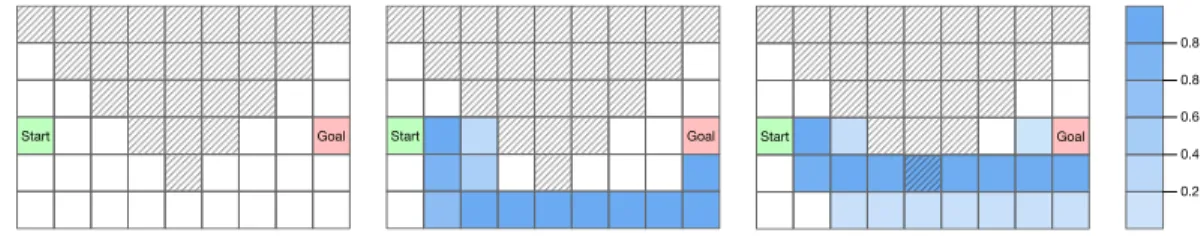
Figure 1: Left: The Risky Mars Rover environment. The agent is required to navigate from the starting point to reach the goal point without staying long (0.5steps in expectation) in the risky area (cross-hatching region). Middle, Right. Example of an optimal mixed policy found by C2RL in a single run. After 10k samples, C2RL finds a mixed policy that randomizes among two policies with weight0.49and0.51. The visitation probabilities of the two policies are plotted.
Theorem 4.5(Memory Complexity Bound). For an constrained RL problem withm-dimensional measurement vector, in the worst case, a mixed policy needs to randomize amongm+ 1individual policies to ensure convergence of RL oracles that search for deterministic policies.
Since the minor cycles in the C2RL method eliminate policies with affinely dependent measurement vectors, after the termination of minor cycles, the size of the active set is at mostm+ 1. That is, the policy found by the C2RL method requires randomization among no more thanm+ 1individual policies. Therefore the proposed C2RL indeed achieves the optimal sparsity in the worst case, making it favorable for large-scale usage.
Corollary 4.5.1. The C2RL method that randomizes among at mostm+ 1policies is worst-case optimal to ensure convergence of any RL oracle.
5
EXPERIMENTS
We evaluate the performance of C2RL in a grid-world navigation task (Fig. 1), and demonstrate its ability to efficiently find sparse policy. In thisRisky Mars Roverenvironment, the agent is required to navigate from the starting point to the goal point, by moving to one of the four neighborhood cells at each step. The episodes terminate when the goal point is reached or after300steps. To enforce robustness, we add a risky area to indicate the dangerous states. The agent receives a measurement vector to indicate the steps it takes (0.1for every step), and whether it stays in the risky area (0.1for every risky step, and0otherwise), with discount factorγ= 0.99. We constrain the agent to reach the goal point with expected cumulative steps measure within1.1and the expected cumulative risky steps within0.05. Note that by design, the shortest path from the starting point to the goal point does not satisfy the constraint. This is common in practice, as robustness typically evolves trade-off between the reward and the constraint satisfaction.
The proposed C2RL method is compared with approachability-based policy optimization (Ap-proPO) (Miryoosefi et al., 2019) and with reward constrained policy optimization (RCPO) (Tessler et al., 2018). ApproPO solves the same convex constrained RL problem by using an RL oracle to play against a no-regret online learner (Hazan et al., 2008; Zinkevich, 2003). Since ApproPO and C2RL both use a RL oracle, ApproPO is a natural baseline to be compared with our method. Besides, we also compare with RCPO, which takes a Lagrangian approach to incorporate the con-straints as a penalty signal into the reward. Using an advantage actor critic (A2C) Mnih et al. (2016), RCPO has been shown to converge to a fixed point. For a fair comparison, C2RL and ApproPO uses an A2C agent as the RL oracle, with the same hyperparameter as used in RCPO. The approximation errors are compared after training for the same number of samples.
Note that the C2RL method does not introduce any extra hyper-parameter. For ApproPO and RCPO, they require extra hyper-parameter for the initialization and learning rate of a variable equivalent to ourλin the outer loop. This is because our approach does not rely on the online learning framework, and therefore there is no need to tune the initialization and learning rate for ourλand ease the usage. We first showcase the consequences of our theoretical results using anoptimal RL oracle. For any
x∈Rm, an optimal policy can be easily found via Dijkstra’s algorithm. If multiple optimal paths
c(⇧⇧)
c( (⇧⇧))
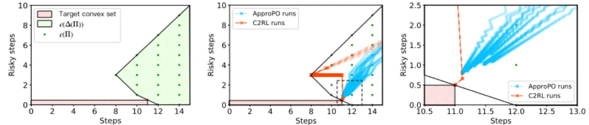
Figure 2: Left: Visualization of the distance minimization problem (7) inR2, where the number
of steps and the number of steps in risky zone are measured. The green hatched region is the polytope formed by values achievable by mixed deterministic policiesc(∆(Π)), and the red hatched region is the target set. Middle: Using anoptimal RL oracle, 10 paths are sampled to showcase the convergence property of C2RL and ApproPO, where each cross on the dashed line corresponds to a call to the oracle.Right: If we zoom in, ApproPO suffers from the zig-zagging problem.
Figure 3: Left: Time complexity measured by number of calling an optimal RL oracle. Middle, Right: Using A2C to approximate an RL oracle, time complexity measured by thousands of samples and memory complexity measured by the number of policies stored are compared.
Using this as an optimal RL oracle, the convergence property of C2RL and ApproPo are compared. Figure 2 Middle shows the value of policiesc(µt)found after each call to the oracle. In Figure 2
Right, when approaching the boundary of the feasible set, the iterations of approachability-based methods start to zigzag. Since C2RL contains a minor cycle to re-optimize the weights among the active set, C2RL progresses quickly to reach the exact optimal solution. In Figure 3 Left, the approximation error is shown for300calls of the optimal RL oracle.
We then compare C2RL, ApproPO and RCPO using the same A2C agent (details of the model structures and hyper-parameters are provided in Appendix E). We run each algorithm for50times, and each run for a maximum of100thousands of samples. The mean and standard deviation of the results are presented in Figure 3. The original paper of ApproPO suggests using a cache to save memory, and the memory requirement of this variant is also presented. Figure 3 demonstrates that C2RL converges to an optimal policy faster than previous methods, and a sparse combination of individual policies is maintained throughout the iteration process.
6
CONCLUSION
In this paper, we introduce C2RL, an algorithm to solve RL problems under orthant or convex constraints. Our method reduces the constrained RL problem to a distance minimization problem, and a novel variant of Frank-Wolfe type algorithm is proposed to solve this. Our method comes with rigorous theoretical guarantees and does not introduce any extra hyper-parameter. To find an-approximation solution, C2RL takesO(1/)calls of any RL oracle and ensures convergence to work with arbitrary RL algorithm. Moreover, C2RL strictly reduces the approximation error between consecutive calls of RL oracle, and form-dimensional constraints, the memory requirement is reduced from storing infinitely many policies (O(1/)) to storing at most constantly many (m+ 1) polices. We further show that the constant is worst-case optimal to ensure the convergence for RL algorithms that search for deterministic policies. Experimentally, we demonstrate that the proposed C2RL method finds sparse solution efficiently, and outperforms previous methods.
REFERENCES
Jacob Abernethy, Peter L Bartlett, and Elad Hazan. Blackwell approachability and no-regret learning are equivalent. InProceedings of the 24th Annual Conference on Learning Theory, pp. 27–46, 2011.
Jacob D Abernethy and Jun-Kun Wang. On frank-wolfe and equilibrium computation. InAdvances in Neural Information Processing Systems, pp. 6584–6593, 2017.
Alekh Agarwal, Alina Beygelzimer, Miroslav Dud´ık, John Langford, and Hanna Wallach. A reduc-tions approach to fair classification.arXiv preprint arXiv:1803.02453, 2018.
Eitan Altman.Constrained Markov decision processes, volume 7. CRC Press, 1999.
Gabriel Barth-Maron, Matthew W Hoffman, David Budden, Will Dabney, Dan Horgan, Dhruva Tb, Alistair Muldal, Nicolas Heess, and Timothy Lillicrap. Distributed distributional deterministic policy gradients. arXiv preprint arXiv:1804.08617, 2018.
Amir Beck and Shimrit Shtern. Linearly convergent away-step conditional gradient for non-strongly convex functions. Mathematical Programming, 164(1-2):1–27, 2017.
Craig Boutilier and Tyler Lu. Budget allocation using weakly coupled, constrained markov decision processes. 2016.
Deeparnab Chakrabarty, Prateek Jain, and Pravesh Kothari. Provable submodular minimization using wolfe’s algorithm. InAdvances in Neural Information Processing Systems, pp. 802–809, 2014.
Minmin Chen, Alex Beutel, Paul Covington, Sagar Jain, Francois Belletti, and Ed H Chi. Top-k off-policy correction for a reinforce recommender system. InProceedings of the Twelfth ACM International Conference on Web Search and Data Mining, pp. 456–464, 2019.
Yinlam Chow and Mohammad Ghavamzadeh. Algorithms for cvar optimization in mdps. In Ad-vances in neural information processing systems, pp. 3509–3517, 2014.
Yinlam Chow, Mohammad Ghavamzadeh, Lucas Janson, and Marco Pavone. Risk-constrained re-inforcement learning with percentile risk criteria.The Journal of Machine Learning Research, 18 (1):6070–6120, 2017.
Yinlam Chow, Ofir Nachum, Edgar Duenez-Guzman, and Mohammad Ghavamzadeh. A lyapunov-based approach to safe reinforcement learning. InAdvances in neural information processing systems, pp. 8092–8101, 2018.
Jes´us A De Loera, Jamie Haddock, and Luis Rademacher. The minimum euclidean-norm point in a convex polytope: Wolfe’s combinatorial algorithm is exponential. InProceedings of the 50th Annual ACM SIGACT Symposium on Theory of Computing, pp. 545–553, 2018.
Miroslav Dud´ık, John Langford, and Lihong Li. Doubly robust policy evaluation and learning.arXiv preprint arXiv:1103.4601, 2011.
Marguerite Frank, Philip Wolfe, et al. An algorithm for quadratic programming. Naval research logistics quarterly, 3(1-2):95–110, 1956.
Yoav Freund and Robert E Schapire. Adaptive game playing using multiplicative weights. Games and Economic Behavior, 29(1-2):79–103, 1999.
Scott Fujimoto, Herke Van Hoof, and David Meger. Addressing function approximation error in actor-critic methods. arXiv preprint arXiv:1802.09477, 2018.
Dan Garber and Elad Hazan. A linearly convergent conditional gradient algorithm with applications to online and stochastic optimization.arXiv preprint arXiv:1301.4666, 2013a.
Dan Garber and Elad Hazan. Playing non-linear games with linear oracles. In 2013 IEEE 54th Annual Symposium on Foundations of Computer Science, pp. 420–428. IEEE, 2013b.
Peter Geibel and Fritz Wysotzki. Risk-sensitive reinforcement learning applied to control under constraints. Journal of Artificial Intelligence Research, 24:81–108, 2005.
Elad Hazan, Alexander Rakhlin, and Peter L Bartlett. Adaptive online gradient descent. InAdvances in Neural Information Processing Systems, pp. 65–72, 2008.
Martin Jaggi. Revisiting frank-wolfe: Projection-free sparse convex optimization. InProceedings of the 30th international conference on machine learning, number CONF, pp. 427–435, 2013. Nan Jiang and Lihong Li. Doubly robust off-policy value evaluation for reinforcement learning. In
International Conference on Machine Learning, pp. 652–661. PMLR, 2016.
Simon Lacoste-Julien and Martin Jaggi. On the global linear convergence of frank-wolfe optimiza-tion variants. InAdvances in neural information processing systems, pp. 496–504, 2015. Hoang Le, Cameron Voloshin, and Yisong Yue. Batch policy learning under constraints. In
Inter-national Conference on Machine Learning, pp. 3703–3712, 2019.
Timothy P Lillicrap, Jonathan J Hunt, Alexander Pritzel, Nicolas Heess, Tom Erez, Yuval Tassa, David Silver, and Daan Wierstra. Continuous control with deep reinforcement learning. arXiv preprint arXiv:1509.02971, 2015.
Sobhan Miryoosefi, Kiant´e Brantley, Hal Daume III, Miro Dudik, and Robert E Schapire. Reinforce-ment learning with convex constraints. InAdvances in Neural Information Processing Systems, pp. 14093–14102, 2019.
BF Mitchell, Vladimir Fedorovich Dem’yanov, and VN Malozemov. Finding the point of a polyhe-dron closest to the origin. SIAM Journal on Control, 12(1):19–26, 1974.
Volodymyr Mnih, Koray Kavukcuoglu, David Silver, Alex Graves, Ioannis Antonoglou, Daan Wier-stra, and Martin Riedmiller. Playing atari with deep reinforcement learning. arXiv preprint arXiv:1312.5602, 2013.
Volodymyr Mnih, Adria Puigdomenech Badia, Mehdi Mirza, Alex Graves, Timothy Lillicrap, Tim Harley, David Silver, and Koray Kavukcuoglu. Asynchronous methods for deep reinforcement learning. InInternational conference on machine learning, pp. 1928–1937, 2016.
Santiago Paternain, Luiz Chamon, Miguel Calvo-Fullana, and Alejandro Ribeiro. Constrained rein-forcement learning has zero duality gap. InAdvances in Neural Information Processing Systems, pp. 7555–7565, 2019.
Doina Precup. Eligibility traces for off-policy policy evaluation. Computer Science Department Faculty Publication Series, pp. 80, 2000.
Doina Precup, Richard S Sutton, and Sanjoy Dasgupta. Off-policy temporal-difference learning with function approximation. InICML, pp. 417–424, 2001.
Richard S Sutton and Andrew G Barto. Reinforcement learning: An introduction. MIT press, 2018. Chen Tessler, Daniel J Mankowitz, and Shie Mannor. Reward constrained policy optimization. In
International Conference on Learning Representations, 2018.
Hado Van Hasselt, Arthur Guez, and David Silver. Deep reinforcement learning with double q-learning.arXiv preprint arXiv:1509.06461, 2015.
Ziyu Wang, Tom Schaul, Matteo Hessel, Hado Hasselt, Marc Lanctot, and Nando Freitas. Dueling network architectures for deep reinforcement learning. InInternational conference on machine learning, pp. 1995–2003, 2016.
Philip Wolfe. Convergence theory in nonlinear programming. Integer and nonlinear programming, pp. 1–36, 1970.
Philip Wolfe. Finding the nearest point in a polytope.Mathematical Programming, 11(1):128–149, 1976.
Shuai Xiao, Le Guo, Zaifan Jiang, Lei Lv, Yuanbo Chen, Jun Zhu, and Shuang Yang. Model-based constrained mdp for budget allocation in sequential incentive marketing. InProceedings of the 28th ACM International Conference on Information and Knowledge Management, pp. 971–980, 2019.
Xiangyu Zhao, Liang Zhang, Long Xia, Zhuoye Ding, Dawei Yin, and Jiliang Tang. Deep rein-forcement learning for list-wise recommendations.arXiv, pp. arXiv–1801, 2017.
Guanjie Zheng, Fuzheng Zhang, Zihan Zheng, Yang Xiang, Nicholas Jing Yuan, Xing Xie, and Zhenhui Li. Drn: A deep reinforcement learning framework for news recommendation. In Pro-ceedings of the 2018 World Wide Web Conference, pp. 167–176, 2018.
Martin Zinkevich. Online convex programming and generalized infinitesimal gradient ascent. In Proceedings of the 20th international conference on machine learning (icml-03), pp. 928–936, 2003.
Lixin Zou, Long Xia, Zhuoye Ding, Jiaxing Song, Weidong Liu, and Dawei Yin. Reinforcement learning to optimize long-term user engagement in recommender systems. In Proceedings of the 25th ACM SIGKDD International Conference on Knowledge Discovery & Data Mining, pp. 2810–2818, 2019.
A
MORE ON
FRANK-WOLFE-TYPE
ALGORITHMS
A.1 STANDARDFRANK-WOLFEALGORITHMAlgorithm 2Frank-Wolfe algorithm (Frank et al., 1956) Input:obj.f :Y 7→R, oracleO(·), init.x0∈ Y
1: fort=1, 2, 3 . . . , Tdo
2: s←Oracle(∇f(xt−1)) = arg mins∈{s1,...,sn}s
T∇f(x t−1) 3: xt←(1−ηt)xt−1+ηts, forηt:= t+22
4: end for 5: returnxT
For a convex functionf : X 7→ Rthe Frank-Wolfe algorithm (FW) solves the constrained
opti-mization problem over a compact and convex setX. The standard FW is known to have a sublinear convergence rate, and various methods are proposed to improve the performance. For example, when the underlying feasible set is a polytope, and the objective function is strongly convex, multi-ple variants, such as away-step FW (Wolfe, 1970; Jaggi, 2013), pairwise FW (Mitchell et al., 1974), and Wolfe’s method (Wolfe, 1976) are shown to enjoy linear convergence rate. Linear convergence under other conditions is also studied (Beck & Shtern, 2017; Garber & Hazan, 2013a;b).
A.2 WOLFE’SMETHOD FORMINIMUMNORMPOINT
Algorithm 3Wolfe’s Method for Minimum Norm Point Initializex∈ P, active setS= [x]and weightλ= [1]. Output:x∈ Pthat has the minimum Euclidean norm.
1: whiletruedo // Major cycle
2: s←Oracle(x) // Potential improving point 3: if||x||2≤xTs+thenbreak
4: S ← S ∪ {s}
5: whiletruedo // Minor cycle
6: y,α←AffineMinimizer(S) //y= arg mins∈aff(S)||s||2
7: ifαs>0for allsthenbreak //y∈conv(S)
8: // Ify∈/ conv(S), then updateyto the intersection ofconv(S)and segment joiningxand
y. Then remove points inSunnecessary for describingy. 9: θ←mini:αi≤0 λi λi−αi // Recallλsatisfiesx= P s∈Sλss 10: y←θy+ (1−θ)x, λi=θαi+ (1−θ)λi 11: S ← {si|si∈ Sandλi>0} 12: end while 13: Updatex=yandλ=α. 14: end while 15: returnx
Wolfe’s method is an iterative algorithm for finding the point with minimum Euclidean norm in a polytope, which is defined as the convex hull of a set of finitely many points.
The Wolfe’s method consists of a finite number of major cycles, each of which consists of a finite number of minor cycles. At the start of each major cycle, let H(x) := {yTx = xx} be the
hyperplane defined byx. IfH(x)separates the polytope from the origin, then the major cycle is terminated. Otherwise, it invokes an oracle to find any point on the near side of the hyperplane. The point is then added into the active setS, and starts a minor cycle.
In a minor cycle, letybe the point of smallest norm in of the affine hull aff(S). Ify is in the relative interior of the convex hullconv(S), thenxis updated toyand the minor cycle is terminated. Otherwise,yis updated to the nearest point toyon the line segmentconv(S)∩[x,y]. Thusyis updated to a boundary point ofconv(S), and any point that is not on the face ofconv(S)in which
whose affine minimizer lies inside its convex hull. Since a set of one point is always a corral, the minor cycles is terminated after a finite number of runs.
B
PROOF OF
THEOREM
4.1
Theorem 4.1 (Approximation Error Strictly Decreases). For any non-terminal step t, we have err(µt+1) < err(µt). That is, the measurement vector of µt found by the C2RL method gets
strictly closer to the convex setΩafter major cycle step.
Proof. If the current step is a major cycle with no minor cycle, thenxt+1is the affine minimizer of aff(S ∪ {st})with respect toωt. Then the affine minimizer property implies(st−xt+1)(xt+1− ωt) = 0. Since iteration does not terminate at stept, we have(xt−ωt)T(xt−st) > 0, and
thereforext+1 not equal to xt. Then xt+1 is the unique affine minimizer impliesf
Ω(xt+1) = minω∈Ω||xt+1−ω||2≤ ||xt+1−ωt||2<||xt−ωt||2=fΩ(xt).
Otherwise the current step contains one or more minor cycles. In this case, we show that the first minor cycle strictly reduces the approximation error, and the (possibly) following minor cycles cannot increase it. For the first minor cycle, the affine minimizery0ofaff(S ∪ {st})with respect
toωtis outsideconv(S ∪ {st}). Letz=θy0+ (1−θ)xtbe the intersection ofconv(S ∪ {st})
and segment joiningxandy. LetV0:=StandVidenote the active set after thei-th minor cycle.
Then sincey1is the affine minimizer ofV1with respect toωt, we have
||z−ωt||=||θy0+ (1−θ)xt−ωt|| ≤θ||y0−ωt||+ (1−θ)||xt−ωt||<||xt−ωt||, (17) where the second step uses the triangle inequality and the last step follows since the segmentxty0
intersects the interior ofconv(S ∪{st}), and the distance toωtstrictly decreases along this segment.
Therefore the pointzfound by first minor cycle satisfies fΩ(z) = min
ω∈Ω||z−ω||
2≤ ||z−ωt||2<||xt−ωt||=f
Ω(xt). (18)
Henceh(y1) < h(xt), and the first minor cycle strictly decreases the approximation error. By a
similar argument, in subsequent minor cycles the approximation error cannot be increased. However, after the first minor cycle, the iterating point may already at the intersection point and the strict inequality in last step of Eq. 17 need to be replaced by non-strict inequality.
Therefore any major cycle either finds an improving point and continue, or enters minor cycles where the first minor cycle finds an improving point, and the subsequent minor cycles does not increase the distance. Adding both side offΩ(xt+1)< fΩ(xt)byfΩ(x∗)and we have the approximation errorh(xt+1)< h(xt)strictly decreases.
C
PROOF OF
THEOREM
4.2
We first prove the Theorem 4.2, using Lemma 4.3 and Lemma 4.4. Then we present the proof of the lemmas.
Theorem 4.2(Convergence in Approximation Error). Fort≥1, the mixed policyµtfound by the
C2RL method satisfies
err(µt)≤16Q2/(t+ 2). (19) whereQ:= maxµ∈∆(U)||c(µ)||is the maximum norm of a measurement vector.
Proof. Since Lemma 4.4 shows that drop steps are no more than half of total major cycle steps, and Theorem 4.1 guarantees these drop steps reducing the approximation error, we can safely skip these step, and re-index the step numbers to include non-drop steps only usingk.
For these non-drop steps, we claim thaterr(µk)≤8Q2/(k+ 1). Using Lemma 4.3, we prove the convergence rate using induction. We first bound the error of anyerr(µk). For anyk≥1
err(µk) = dist2(c(µk),Ω)− dist2(c(µ∗),Ω) (20) = 1/2||c(µk)− ProjΩ(c(µk))||2−1/2||c(µ∗)− ProjΩ(c(µ∗))||2 (21) ≤1/2(||c(µk)||2+||ProjΩ(c(µk))||2− ||c(µ∗)||2− ||ProjΩ(c(µ∗))||2) (22) ≤ ||c(µk)||2− ||c(µ∗)||2 (23) ≤ ||c(µk)||2 (24) ≤Q2, (25)
where Eq. 21 uses the definition of our squared Euclidean distance function. Eq. 22 follows from triangle inequality, and Eq. 23 is by the contractive property of the Euclidean distance.
Whenk = 1, the Eq. 25 established the based case. Now fork ≥ 1, assume that err(µk) ≤
8Q2/(k+ 1)for k ≥ 1, then Lemma 4.3 giveserr(µk+1) ≤err(µk)−err2(µk)/8Q2. Since the quadratic function of the right hand side is monotonically increasing on(−∞,4Q2], using the inductive hypothesis
err(µk+1)≤err(µk)−
err2(µk)/8Q2≤8Q2/(k+ 1)−8Q2/(k+ 1)2≤Q2/(k+ 2) (26) Since fort steps of major cycle steps, the number of non-drop stepsk > t/2, we conclude that err(µt)≤16Q2/(t+ 2).
Then we prove the lemmas.
Lemma 4.3. For a non-drop step, we haveerr(µt)−err(µt+1)≥err2(µt)/8Q2.
Proof. The non-drop step contains either no minor cycle or one minor cycle. We first consider the no minor cycle case.
If a major cycle contains no minor cycle, thenxt+1is the affine minimizer of theS ∪ {st}.
err(µt)−err(µt+1) =dist2(xt,Ω)−dist2(xt+1,Ω) (27) = 1/2(||xt−ωt||2−min ω∈Ω||x t+1 −ω||2) (28) ≥1/2(||xt−ωt||2− ||xt+1−ωt||2) (29) = 1/2(||xt−ωt||2+||xt+1−ωt||2−2||xt+1−ωt||2) (30) = 1/2(||xt−ωt||2+||xt+1−ωt||2−2(xt−ωt)T(xt+1−ωt)) (31) = 1/2(||xt−xt+1||2), (32)
where the equation (31) follows from the affine minimizer property Eq. (11). For||xt−xt+1||in the last equation, and∀q∈aff(S ∪ {st}), we have
||xt−xt+1|| ≥ ||xt−xt+1||||x t||+||q|| 2Q (Definition ofQ) (33) ≥ ||xt−xt+1||||x t−q|| 2Q (Triangle inequality) (34) ≥ 1 2Q(x t−xt+1)(xt−q) (Cauchy-Schwarz inequality) (35) = 1 2Q(x
t−ωt)(xt−q) (Affine minimizer property). (36)
SinceΩis a convex set, the squared Euclidean distance functiondist2(x,Ω)is convex forx, which implies
dist2(xt,Ω) + (q−xt)∇dist2(xt,Ω)≤dist2(q,Ω). (37) Putting in∇dist2(xt,Ω) = (xt−ProjΩ(xt)) = (xt−ωt), we get(xt−ωt)(xt−q)≥err(µt),
which together with Eq. 32 and Eq. 36 concludes that for non-drop step with no minor cycles, we haveerr(µt)−err(µt+1)≥
err2(µt)/8Q2.
For non-drop step with one minor cycle, we use the Theorem 6 of (Chakrabarty et al., 2014). By a linear translation of adding all points with−ωt, it gives
||xt−ωt||2− ||xt+1−ωt||2≥((xt−ωt)(xt−q))2/8Q2. (38) Then applying the same argument as Eq. 37, and we finished our proof.
Lemma 4.4. Aftertmajor cycle steps of C2RL method, the number of drop steps is less thant/2. Proof. Recall that at the termination of a minor cycle, the size of the active set|Sc| ∈[1, m]. Since in each major cycle steps, the size of active setStincreases by one, and each drop step reduces the size ofStby at least one, the number of drop steps is always less than half of total number of the major cycle steps.
D
PROOF OF
THEOREM
4.5
Theorem 4.5(Memory Complexity Bound). For an constrained RL problem withm-dimensional measurement vector, in the worst case, a mixed policy needs to randomize amongm+ 1individual policies to ensure convergence of RL oracles that search for deterministic policies.
Proof. We give a constructive proof. Consider am-dimensional vector-valued MDP with a sin-gle state,m+ 1actions, andc(ai) := ei is the unit vector ofi-th dimension fori ∈ [1, m], and c(am+1) := 0, and the episode terminates after1steps. The constrained RL problem is to find a policy whose measurement vector lies in the convex set of a single point{1/2m}. By linear pro-gramming, it is clear that the only feasible mixed deterministic policy is to selectam+1with1/2 probability, and the restmactions with 1/2mprobability; i.e. the unique feasible policy to this problem has an active set containingm+ 1deterministic policies. Therefore any method random-ize among less than m+ 1individual policies does not ensure convergence when used with RL algorithms searching for deterministic policies.
E
ADDITIONAL
EXPERIMENT
DETAILS
All the methods use the same A2C agent. The input is the one-hot encoded current position index. The A2C is the standard fully connected multi-layer perceptron with ReLU activation function. The actor and critic share the internal representation and have their only final layer. Both actor and critic networks use Adam optimizer with learning rate set to1e−2. The network is as follows
Actor Critic
Input layer One-hot encoded state index (dim=54) Hidden layer Linear(in=54, out=128, act=”relu”)
Output layer Linear(in=128, out=4, act=”relu”) Linear(in=128, out=1, act=”relu”)
Output name Action score State value
For ApproPO, the constant κfor projection convex set to convex cone is set to be20. The θ is initialized to0. Following the original paper.
For RCPO, the learning rate of itsλis set to2.5e−5, and itsλis initialized to0and updated by online gradient descent with learning rate set to1, as used by the original paper.