A Linear Programming Based Method for Job Shop Scheduling

Kerem B ¨ulb ¨ul

Sabancı University, Manufacturing Systems and Industrial Engineering, Orhanlı-Tuzla, 34956 Istanbul, Turkey [email protected]

Philip Kaminsky

Industrial Engineering and Operations Research, University of California, Berkeley, CA [email protected]

Abstract: We present a decomposition heuristic for a large class of job shop scheduling problems. This heuristic

utilizes information from the linear programming formulation of the associated optimal timing problem to solve subproblems, can be used for any objective function whose associated optimal timing problem can be expressed as a linear program (LP), and is particularly effective for objectives that include a component that is a function of individual operation completion times. Using the proposed heuristic framework, we address job shop schedul-ing problems with a variety of objectives where intermediate holdschedul-ing costs need to be explicitly considered. In computational testing, we demonstrate the performance of our proposed solution approach.

Keywords: job shop; shifting bottleneck; intermediate inventory holding costs; non-regular objective; optimal timing

problem; linear programming; sensitivity analysis; single machine; earliness/tardiness.

1. Introduction The job shop scheduling problem, in which each job in a set of orders requires processing on a unique subset of available resources, is a fundamental operations research problem, encompassing many additional classes of problems (single machine scheduling, flow shop scheduling, etc). While from an application perspective this model is traditionally used to sequence jobs in a factory, it is in fact much more general than this, as the resources being allocated can be facilities in a logistics network, craftsmen on a construction job site, etc. In light of both the practical and academic importance of this problem, many researchers have focused on various approaches to solving it. Exact optimization methods, however, have in general proved effective only for relatively small problem instances or simplified versions of the problem (certain single-machine and two-machine flow shop models, for example). Thus, in many cases, researchers who wish to use approaches more sophisticated than simple dispatch rules have been motivated to focus on heuristics for practically sized problem instances, typically metaheuristics (seeLaha(2007) andXhafa and Abraham(2008) and the references therein) or decomposition methods (seeOvacik and Uzsoy(1996) and the references therein). In almost all of this work, however, the objective is a function of the completion time of each job on its final machine, and is not impacted by the completion times of intermediate operations.

This is a significant limitation because objectives that are only a function of job completion times rather than a function of all operation completion times ignore considerations that are increasingly important as the focus on lean, efficient supply chains grows. For example, in many cases, intermediate inventory holding costs are an important cost driver, especially when entire supply chains are being modeled. Often, substantial value is added between processing stages in a production network, but intermediate products may be held in inventory for significant periods of time waiting for equipment to become available for the next processing or transfer step. Thus, in this case, significant savings may result from schedules that delay intermediate processing steps as much as possible. On the other hand, sometimes it makes sense for certain intermediate processing steps to be expedited. Consider, for example, processes when steel must be coated as soon as possible to delay corrosion, or when intermediates are unstable and degrade over time. Indeed, some supply chains and manufacturing processes may have certain steps that have to be expedited and other steps that have to be delayed in order to minimize costs.

Similarly, consider the so-called “rescheduling problem.” Suppose that a detailed schedule exists, and all necessary arrangements have been made to accommodate that schedule. When a supply chain disruption of some kind occurs, so that the schedule has to be changed to account for changing demand or alternate resource availability, the impact of these changes can often be minimized if the new schedule

adheres as closely as possible to the old schedule. This can be accomplished by penalizing operations on machines that start at different times than those in the original schedule.

In these cases and others, a scheduling approach that considers only functions of the completion time of the job, even those that consider finished goods inventory holding cost (e.g., earliness cost) or explicitly penalize deviation from a targeted job completion time, may lead to a significantly higher cost solution than an approach that explicitly considers intermediate holding costs. We refer the reader to

Bulbul(2002) andBulbul et al.(2004) for further examples and a more in-depth discussion.

Unfortunately, the majority of previous work in this area (and of scheduling work in general) focuses on algorithms or approaches that are specific to an individual objective function, and are not adaptable to other objective functions in a straightforward way. Because each approach is highly specialized for a particular objective, it is difficult for a researcher or user to generalize insights for a particular approach to other objectives, and thus from an application point of view, software to solve scheduling problems is highly specialized and customized, and from a research point of view, scheduling research is fragmented. Indeed, published papers, algorithms, and approaches typically focus on a single objective: total completion time, flowtime, or tardiness, for example. It is quite uncommon to find an approach that is applicable to more than one (or one closely related set) of objectives.

Thus, there is a need for an effective, general approach to solve the growing class of scheduling prob-lems that explicitly considers the completion time of intermediate operations. In this paper we address this need by developing an efficient, effective heuristic algorithmic framework useful for addressing job shop scheduling problems for a large class of objectives where operation completion times have a direct impact on the total cost. To clarify the exposition, we present our results in the context of explicitly min-imizing intermediate holding costs, although our approach applies directly and without modification to other classes of problems where operation completion times are critical. This framework builds on the notion of theoptimal timing problemfor a job shop scheduling problem. For any scheduling problem where intermediate holding costs are considered, the solution to the problem is not fully defined by the sequence of operations on machines – it is necessary to specify the starting time of each operation on each machine, since the time that each job is idle between processing steps dictates intermediate holding costs. The problem of determining optimal start times of operations on machines given the sequence of operations on machines is known as the optimal timing problem, and for many job shop scheduling problems, this optimal timing problem can be expressed as an LP.

Specifically,our algorithm applies to any job shop scheduling problem with operation completion time-related costs and any objective for which the optimal timing problem can be expressed as an LP. As we will see, this includes, but is certainly not limited to, objectives that combine holding costs with total weighted completion time, total weighted tardiness, and makespan.

Our algorithm is a machine-based decomposition heuristic related to theshifting-bottleneckheuristic, an approach that was originally developed for the job shop makespan problem byAdams et al.(1988). Versions of this approach have been applied to job shop scheduling problems with maximum lateness (Demirkol et al.(1997)) and total weighted tardiness minimization objectives (Pinedo and Singer(1999),

Singer (2001) and Mason et al. (2002)). None of these authors consider operation completion time-related costs, however, and each author presents a version of the heuristic specific to the objective they are considering. Our approach is general enough to encompass all of these objectives (and many more) combined with operation completion time-related costs. In addition, we believe and hope that other researchers can build on our ideas, particularly at the subproblem level, to further improve the effectiveness of our proposed approach.

In general, relatively little research exists on multi-machine scheduling problems with intermediate holding costs, even those focusing on very specific objectives. Avci and Storer (2004) develop eff ec-tive local search neighborhoods for a broad class of scheduling problems that includes the job shop total weighted earliness and tardiness (E/T) scheduling problem. Work-in-process inventory holding costs have been explicitly incorporated inPark and Kim(2000),Kaskavelis and Caramanis(1998), and

Chang and Liao (1994) for various flow- and job shop scheduling problems, although these papers present approaches for very specific objective functions that do not fit into our framework, and use very different solution techniques. Ohta and Nakatanieng(2006) considers a job shop in which jobs must complete by their due dates, and develops a shifting bottleneck-based heuristic to minimize holding

costs. Thiagarajan and Rajendran(2005) andJayamohan and Rajendran(2004) evaluate dispatch rules for related problems. In contrast, our approach applies to a much broader class of job shop scheduling problems.

2. Problem Description In the remainder of the paper, we restrict our attention to the job shop scheduling problem with intermediate holding costs in order to keep the discussion focused. However, we reiterate that many other job shop scheduling problems would be amenable to the proposed solution framework as long as their associated optimal timing problems are LP’s.

Consider a non-preemptive job shop withmmachines andnjobs, each of which must be processed on a subset of those machines. The operation sequence of job jis denoted by an ordered setMjwhere

theith operation inMjis represented byoij, i= 1, . . . ,mj =| Mj |, and Ji is the set of operations to be

processed on machinei. For clarity of exposition, from now on we assume that theith operationoijof

job jis performed on machineiin the definitions and model below. However, our proposed solution approach applies to general job shops, and for our computational testing we solve problems with more general routing.

Associated with each job j, j=1, . . . ,n, are several parameters: pij, the processing time for job jon

machinei;rj, the ready time for jobj; andhij, the holding cost per unit time for jobjwhile it is waiting in

the queue before machinei. All ready times, processing times and due dates are assumed to be integer. For a given scheduleS, letwijbe the time jobjspends in the queue before machinei, and letCijbe the

time at which job jfinishes processing on machinei. We are interested in objective functions with two components, each a function of a particular schedule: an intermediate holding cost componentH(S), and aC(S) that is a function of the completion times of each job. The intermediate holding cost component can be expressed as follows:

H(S)= n ∑ j=1 mj ∑ i=1 hijwij.

Before detailing permissibleC(S) functions, we formulate them-machine job shop scheduling problem (Jm): (Jm) min H(S)+C(S) (1) s.t. C1j−w1j=rj+p1j ∀j (2) Ci−1j−Cij+wij=−pij i=2, . . . ,mj, ∀j (3) Cik−Cij≥pikorCij−Cik≥pij ∀i,∀j,k∈Ji (4) Cij,wij≥0 i=1, . . . ,mj,∀j. (5)

Constraints (2) prevent processing of jobs before their respective ready times. Constraints (3), referred to as operation precedence constraints, prescribe that a jobjfollows its processing sequenceo1j, . . . ,omjj.

Machine capacity constraints (4) ensure that a machine processes only one operation at a time, and an operation is finished once started. Observe that even if the objective function is linear, due to constraints (4) the formulation is not linear (without a specified order of operations).

The technique we present in this paper is applicable to any objective functionC(S) that can be modeled as a linear objective term along with additional variables and linear constraints added to formulation (Jm). Although this allows a rich set of possible objectives, to clarify our exposition, for our computational experiments we focus on a specific formulation that we call (Jmc) that models total weighted earliness, total weighted tardiness, total weighted completion time, and makespan objectives. For this formulation, in addition to the parameters introduced above,djrepresents the due date for job j;ϵjis the earliness

cost per unit time if job jcompletes its final operation before timedj; πj represents the tardiness cost

per unit time if job jcompletes its final operation after timedj; andγrepresents the penalty per unit

time associated with the makespan. VariablesEjandTjmodel the earliness, max(dj−Cmjj,0), and the

tardiness, max(Cmjj−dj,0), of jobj, respectively. Consequently, the total weighted earliness and tardiness

are expressed as∑jϵjEjand

∑

jπjTj, respectively. Note that ifdj =0∀j, thenTj =Cj∀j, and the total

weighted tardiness reduces to the total weighted completion time. The variableCmax represents the

Formulation (Jmc), which we present below, thus extends formulation (Jm) with additional variables and constraints. Constraints (7) relate the completion times of the final operations to the earliness and tardiness values, and constraints (8) ensure that the makespan is correctly identified.

(Jmc) min n ∑ j=1 mj ∑ i=1 hijwij+ n ∑ j=1 (ϵjEj+πjTj)+γCmax (6) s.t. (2)−(5) Cmjj+Ej−Tj=dj ∀j (7) Cmjj−Cmax+sj=0 ∀j (8) Ej,Tj,sj≥0 ∀j (9) Cmax≥0. (10)

Following the three field notation ofGraham et al.(1979),Jm/rj/∑n_j=1∑mj_i=1hijwij+

∑n

j=1(ϵjEj+πjTj)+ γCmaxrepresents problem (Jmc). (Jmc) is stronglyNP-hard, as a single-machine special case of this problem

with all inventory holding and earliness costs and the makespan cost equal to zero, i.e., the single-machine total weighted tardiness problem 1/rj/∑πjTj, is known to be stronglyNP-hard (Lenstra et al.(1977)).

In the next section of this paper, Section 3, we explain our heuristic for this model. The core of our solution approach is the single-machine subproblem developed conceptually in Section3.3.1and analyzed in depth in AppendixA. In Section4, we extensively test our heuristic, and compare it to the current best approaches for related problems. Finally, in Section5, we conclude and explore directions for future research.

3. Solution Approach As mentioned above, we propose a shifting bottleneck (SB) heuristic for this problem, and our algorithm makes frequent use of the optimal timing problem related to our problem, and is best understood in the context of the disjunctive graph representation of the problem, so in the next two subsections, we review these. For reasons that will become clear in Section3.3.1, we refer to our SB heuristic as the Shifting Bottleneck Heuristic Utilizing Timing Problem Duals (SB-TPD).

3.1 The Timing Problem Observe that (Jm) with a linear objective function would be an LP if we knew the sequence of operations on each machine (which would imply that we could pre-select one of the terms in constraint (4) of (Jm)). Indeed, researchers often develop two-phase heuristics for similar problems based on this observation, where first a processing sequence is developed, and then idle time is inserted by solving the optimal timing problem.

For our problem, once operations are sequenced, and assuming operations are renumbered in se-quence order on each machine, the optimal schedule is obtained by solving the associated timing prob-lem (TTJm), defined below. The variableiijdenotes the time that operationjwaits before processing on

machinei(that is, the time between when machineicompletes the previous operation, and the time that operationjbegins processing on machinei) .

(TTJm) min H(S)+C(S) (11)

s.t.

(2),(3),(5)

Cij−1−Cij+iij=−pij ∀i,j∈Ji,j,1 (12)

iij≥0 ∀i,j∈Ji,j,1 (13)

Specifically, in our approach, we construct operation processing sequences by solving the subproblems of a SB heuristic. Once the operation processing sequences are obtained, we find the optimal schedule given these sequences by solving (TTJm). The linear program (TTJm) hasO(nm) variables and constraints. As mentioned above, to illustrate our approach, we focus on a specific example, (Jmc). The timing problem for (Jmc), (TTJm[), follows. (TTJm[) min n ∑ j=1 mj ∑ i=1 hijwij+ n ∑ j=1 (ϵjEj+πjTj)+γCmax (14)

s.t.

(2),(3),(5) (7)−(10) (12)−(13)

Also, for some of our computational work, it is helpful to add two additional constraints to formulation (TTJm[), Cmax≤CUBmax (15) n ∑ j=1 πjTj≤WTUB, (16) whereCUB

maxandWTUBare upper bounds onCmaxand the total weighted tardiness, respectively. 3.2 Disjunctive Graph Representation The disjunctive graph representation of the scheduling problem plays a key role in the development and illustration of our algorithm. Specifically, the dis-junctive graph representationG(N,A) for an instance of our problem is given in Figure1, where the machine processing sequences for jobs 1, 2, 3 are given byM1 = {o11,o31,o21}, M2 = {o22,o12,o32}, and

M3 = {o23,o13,o33}, respectively. There are three types of nodes in the node setN: one node for each

operationoij, one dummy starting nodeSand one dummy terminal nodeT, and one dummy terminal

nodeFjper job associated with the completion of the corresponding jobj. The arc setAconsists of two

types of arcs: the solid arcs in Figure1represent the operation precedence constraints (3) and are known as conjunctive arcs. The dashed arcs in Figure1are referred to as disjunctive arcs, and they correspond to the machine capacity constraints (4).

0 p22 p12 p32 p23 p13 p33 r1 p11 p31 p21 r2 r3

S

o

o

o

o

o

o

o

o

o

F

F

F

T

Figure 1: Disjunctive graph representation for (Jm).

Before a specific schedule is determined for a problem, there is initially a pair of disjunctive arcs between each pair of operations on the same machine (one in each direction). The set of conjunctive and disjunctive arcs are denoted byACandAD, respectively, and we haveA=AC∪AD. Both conjunctive and

disjunctive arcs emanating from a nodeoijhave a length equal to the processing timepijof operationoij.

The ready time constraints (2) are incorporated by connecting the starting nodeSto the first operation of each job jby an arc of lengthrj. The start time of the dummy terminal nodeTmarks the makespan.

A feasible sequence of operations for (Jm) corresponds to a selection of exactly one arc from each pair of disjunctive arcs (also referred to as fixing a pair of disjunctive arcs) so that the resulting graph G′(N,AC∪A_DS) is acyclic whereAS_Ddenotes the set of disjunctive arcs included inG′. However, recall that

by itself, this fixing of disjunctive arcs does not completely describe a schedule for (Jm). The operation completion times and the objective value corresponding toG′are obtained by solving (TTJm) where the constraints (12) corresponding toAS

Dare included. Note that a disjunctive arc (oij,oik)∈ASDcorresponds

to a constraintCij−Cik+iik=−pikin (TTJm).

3.3 Key Steps of the Algorithm SB-TPD is an iterative machine-based decomposition algorithm.

• First, a disjunctive graph representation of the problem is constructed. Initially, there are no machines scheduled, so that no disjunctive arcs are fixed, i.e., AS

machine capacity constraints are initially ignored, and the machines are in effect allowed to process as many operations as required simultaneously.

• At each iterationof SB-TPD, one single-machine subproblem is solved for each unscheduled machine (we detail the single-machine subproblem below), the “bottleneck machine” is selected from among these (we detail bottleneck machine selection below), and the disjunctive arcs corresponding the schedule on this “bottleneck machine” are added to AS

D. As we discuss

below, the disjunctive graph is used to characterize single-machine problems at each iteration of the problem, and to identify infeasible schedules. Finally, the previous scheduling decisions are re-evaluated, and some machines are re-scheduled if necessary.

• These steps are repeateduntil all machines are scheduled and a feasible solution to the problem (Jm) is obtained.

• A partial tree searchover the possible orders of scheduling the machines performs the loop in the previous steps several times. Multiple feasible schedules for (Jm) are obtained and the best one is picked as the final schedule produced by SB-TPD.

In the following subsections, we provide more detail.

3.3.1 The Single-Machine Problem The key component of any SB algorithm is defining an appro-priate single-machine subproblem. The SB procedure starts with no machine scheduled and determines the schedule of one additional machine at each iteration. The basic rationale underlying the SB proce-dure dictates that we select the machine that hurts theoverallobjective the most as the next machine to be scheduled, given the schedules of the currently scheduled machines. Thus, the single-machine subproblem defined must capture accurately the effect of scheduling a machine on the overall objective function. In the following discussion, assume that the algorithm is at the start of some iteration, and let

MandMS⊂ Mdenote the set of all machines and the set of machines already scheduled, respectively. Since “machines being scheduled” corresponds to fixing disjunctive arcs, observe that at this stage of the algorithm, the partial schedule is represented by disjunctive graphG′(N,AC∪AS_D) whereAS_Dcorresponds

to the selection of disjunctive arcs fixed for the machines inMS.

In our problem, the overall objective function value and the corresponding operation completion times are obtained by solving (TTJm). The formulation given in (11)-(13) requires all machine sequences to be specified. However, note that we can also solve an intermediate version of (TTJm) – one that only includes machine capacity constraints corresponding to the machines inMS_{while omitting the capacity}

constraints for the remaining machines inM \ MS_{. We refer to this intermediate optimal timing problem}

and its optimal objective value as (TTJm)(MS_{) andz}

(TTJm)(MS), respectively, and say that (TTJm) is

solved over the disjunctive graphG′(N,AC∪AS_D).

Observe that initially SB-TPD starts with no machine scheduled, i.e.,MS_{is initially empty. Therefore,}

at the initialization step (TTJm) is solved over a disjunctive graphG′(N,AC∪AS_D) whereAS_D = ∅ by

excluding all machine capacity constraints (12) and yields a lower bound on the optimal objective value of the original problem (Jm).

Once again, assume that algorithm is at the start of an iteration, so that a set of machines MS

is already scheduled and the disjunctive arcs selected for these machines are included in AS D. The

optimal completion times C∗_ij for all i ∈ M and j ∈ Ji are also available from (TTJm)(MS) . As the

current iteration progresses, a new bottleneck machineib_{must be identified by determining which of}

the currently unscheduled machinesi∈ M \ MS_{will have the largest impact on the objective function}

of (TTJm)(MS_{∪i) if it is sequenced effectively (that is, in the way that minimizes its impact). Then,}

a set of disjunctive arcs for machineib_{corresponding to the sequence provided by the corresponding}

subproblem is added toAS

D, and a new set of optimal completion timesC′ij for alli ∈ Mand j ∈ Ji is

determined by solving (TTJm)(MS_{∪ {i}b_}).

Clearly, the optimal objective value of (TTJm)(MS∪ {ib_{}) is no less than that of (TTJm)(M}S_{), i.e.,}

z(TTJm)(MS∪ {ib}) ≥ z(TTJm)(MS) must hold. Therefore, a reasonable objective for the subproblem of

machineiis to minimize the differencez(TTJm)(MS∪ {i})−z(TTJm)(MS). In the remainder of this section,

we show how this problem can be solved approximately as a single-machine E/T scheduling problem with distinct ready times and due dates.

For defining the subproblem of machine i, we note that if the completion times obtained from (TTJm)(MS_{) for the set of operations J}

i to be performed on machine i are equal to those obtained

from (TTJm)(MS_{∪ {i}) after adding the corresponding machine capacity constraints, i.e., ifC}∗

ij=C′ijfor

all j∈ Ji, then we havez(TTJm)(MS)=z(TTJm)(MS∪ {i}). This observation implies that we can regard the

current operation completion timesC∗_ijprovided by (TTJm)(MS) as due dates in the single-machine sub-problems. Early and late deviations from these due dates are discouraged by assigning them earliness and tardiness penalties, respectively. These penalties are intended to represent the impact on the overall problem objective if operations are moved earlier or later because of the way a machine is sequenced.

Specifically, for a machine i ∈ M \ MS_{, some of the operations in J}

i may overlap in the optimal

solution of (TTJm)(MS) because this timing problem excludes the capacity constraints for machinei. Thus, scheduling a currently unscheduled machineiimplies removing the overlaps among the operations on this machine by moving them earlier/later in time. This, of course, may also affect the completion times of operations on other machines. For a given operationoijon machinei, assume thatC∗_ij =dijin

the optimal solution of (TTJm)(MS). Then, we can measure the impact of moving operationoijforδ >0

time units earlier or later on the overall objective function by including a constraint of the form

Cij+sij=dij−δ (Cij≤dij−δ) or (17)

Cij−sij=dij+δ (Cij≥dij+δ), (18)

respectively, in the optimal timing problem (TTJm)(MS_{) and resolving it, where the variable s} ij ≥

0 denotes the slack or surplus variable associated with (17) or (18), respectively, depending on the context. Of course, optimally determining the impact on the objective function for all values of δ is computationally prohibitive as we explain later in this section. However, as we demonstrate in AppendixA, the increase in the optimal objective value of (TTJm)(MS_{) due to an additional constraint}

(17) or (18) can be bounded by applying sensitivity analysis to the optimal solution of (TTJm)(MS_{) to}

determine the value of the dual variables associated with the new constraints. Specifically, we show the following:

Proposition3.1 Consider the optimal timing problems(TTJm)(MS)and(TTJm)(MS∪{ib})solved in iterations

k and k+1of SB-TPD where ib_{is the bottleneck machine in iteration k. For any operation o} ib_j, if C′

ib_j=Cib_j−δ

or C′_ib_j=Cib_j+δfor someδ >0, then z₍TTJm)(MS∪ {ib})−z(TTJm)(MS)≥|y¯_m′′₊₁ |δ≥0,wherey¯′′is defined in

AppendixAin(36)-(37). ¯

y′′_m+1is the value of the dual variable associated with (17) or (18) if we augment (TTJm)(MS) with (17) or (18), respectively, and carry out a single dual simplex iteration. Thus, the cost increase characterized in Proposition3.1is in some ways related to the well-known shadow price interpretation of the dual variables. In AppendixA, we give a closed form expression for ¯y′′that can be calculated explicitly using only information present in the optimal basic solution to (TTJm)(MS_{). Thus, we can efficiently bound}

the impact of pushing an operation earlier or later by δ time units on the overall objective function from below. This allows us to formulate the single-machine subproblem of machineiin SB-TPD as a single-machine E/T scheduling problem 1/rj/∑ϵjEj+πjTjwith the following parameters: the ready

timerijof jobjon machineiis determined by the longest path from nodeSto nodeoijin the disjunctive

graphG′(N,AC∪AS_D); the due datedijof jobjon machineiis the optimal completion timeC∗_ijof operation

oijin the current optimal timing problem (TTJm)(MS); the earliness and tardiness costsϵijandπijof job

jon machineiare given by

ϵij=−y¯′′_m+1= _¯¯ct Ajt =− max k,j|A¯jk>0 ¯ ck −_A¯_jk and πij=y¯′′m+1=− ¯ ct ¯ Ajt =−max k|A¯jk<0 ¯ ck ¯ Ajk , (19)

respectively, where these quantities are defined in (34) and (36)-(37). (IfC∗_ij = rij+pij, then it is not

feasible to push operation oij earlier, and ϵij is set to zero.) As we detail in Appendix A, this cost

function, developed for shifting a single operationoijearlier or later, is based on a single implicit dual

simplex iteration after adding the constraint (17) or (18) to (TTJm)(MS_{). We are therefore only able} to obtain a lower boundon the actual change in cost that would result from changing Cij from its

current valueC∗_ij. In general, the amount of change in cost would be a piecewise linear and convex function as illustrated in Figure2. However, while the values ofϵijandπijin (19) may be computed

efficiently based on the current optimal basis of (TTJm)(MS_{) – see AppendixBfor an example on (TTJm}[₎

–, we detail at the end of AppendixAhow determining the actual cost functions requires solving one LP with a parametric right hand side for each operation, and is therefore computationally expensive. In addition, the machine capacity constraints are introduced simultaneously for all of the operations on the bottleneck machine in SB-TPD, and there is no guarantee that this combined effect is close to the sum of the individual effects. However, as we demonstrate in our computational experiments in Section4, the single-machine subproblems provide reasonably accurate bottleneck information and lead to good operation processing sequences. We also note that the single-machine E/T scheduling problem 1/rj/∑ϵjEj+πjTjis strongly NP-hard because a special case of this problem with all earliness costs

equal to zero, i.e., the single-machine total weighted tardiness problem 1/rj/∑πjTj, is stronglyNP-hard

due toLenstra et al.(1977). Several efficient heuristic and optimal algorithms have been developed for 1/rj/∑ϵjEj+πjTjin the last decade. SeeBulbul et al.(2007),Tanaka and Fujikuma(2008),Sourd(2009), Kedad-Sidhoum and Sourd(2010). Our focus here is to develop an effective set of cost coefficients for the subproblems, and any of the available algorithms in the literature could be used in conjunction with the approach we present. For the computational experiments in Section4, in some instances we solve the subproblem optimally using a time-indexed formulation, and in some instances we solve the subproblem heuristically using the algorithm ofBulbul et al.(2007). The basis of this approach is constructing good operation processing sequences from a tight preemptive relaxation of 1/rj/∑ϵjEj+πjTj. We note that

it is possible to extend this preemptive lower bound to a general piecewise linear and convex E/T cost function with multiple pieces on either side of the due date. Thus, if one opts for constructing the actual operation cost functions explicitly at the expense of extra computational burden, it is possible to extend the algorithm ofBulbul et al.(2007) to solve the resulting subproblems.

approximation

actual

C

ϵ

π

d

=

C

Figure 2: Effect of moving a single operation on the overall objective.

Also, an additional difficulty might arise at each iteration of the algorithm. We observe that when the set of disjunctive arcs in the graphG′(N,AC∪AS_D) is empty, then no path exists between any two

operationsoik andoij on a machinei ∈ M. However, as we add disjunctive arcs toG′, we may create

paths between some operations of a currently unscheduled machinei<MS_{. In particular, a path from}

node oik tooij indicates a lower bound on the amount of time that must elapse between the starting

times of these two operations. This type of path is an additional constraint on the final schedule, and is referred to as a delayed precedence constraint (DPC). Rather than explicitly incorporate these DPC’s into our subproblem definition, we check for directed cycles while updatingG′, since violated DPC’s imply cycles in the updated graph. If necessary, we remove cycles by applying local changes to the sequence of the current bottleneck machine.

We conclude this section with some comments on classical job shop scheduling problems with regular objective functions, such as Jm//Cmax, Jm//∑jwjCj, and Jm//∑jwjTj. The cost coefficients in (19)

measure the marginal effect of moving operationoijearlier or later. The former is clearly zero for any

regular objective function. Furthermore,πijis also zero if the job completion time is not affected by a marginal delay in the completion time ofoij. Thus, SB-TPD may be ineffective for the classical objectives in

the literature. The true benefits of our solution framework are only revealed when operation completion times have a direct impact on the total cost. Furthermore, for regular objectives, the task of estimating the actual piecewise linear operation cost functions is accomplished easily by longest path calculations in the disjunctive graph. Of course, solving the resulting single-machine subproblems with a general piecewise linear and convex weighted tardiness objective is a substantially harder task. Bulbul(2011) formalizes these concepts and develops a hybrid shifting bottleneck-tabu search heuristic for the job shop total weighted tardiness problem by generalizing the algorithm ofBulbul et al.(2007) for solving the subproblems as discussed above.

3.3.2 Selecting the Bottleneck Machine As alluded to above, at each iteration of the algorithm, we solve the single-machine problem described abovefor each of the remaining unscheduled machines, and select the one with the highest corresponding subproblem objective value to be the current bottleneck machineib_{. Then, the disjunctive graph and the optimal timing problem are updated accordingly to}

include the machine capacity constraints of this machine where the sequence of operations onib _are

determined by the solution of the corresponding subproblem.

3.3.3 Rescheduling The last step of an iteration of SB-TPD is re-evaluating the schedules of the previously scheduled machines inMS_{given the operation processing sequence on the current bottleneck}

machineib_{. It is generally observed that SB algorithms without a rescheduling step perform rather poorly}

(Demirkol et al.(1997)). We perform a classical rescheduling step, such as that in Pinedo and Singer

(1999). For each machine i ∈ MS_{, we first delete the corresponding disjunctive arcs from the set}

AS_D and construct a subproblem for machinei based on the solution of the optimal timing problem

(TTJm)(MS\ {i} ∪ {ib}). Then, machine iis re-scheduled according to the sequence obtained from the

subproblem by adding back the corresponding disjunctive arcs toAS

D. The rescheduling procedure may

be repeated several times until no further improvement in the overall objective is achieved.

3.3.4 Tree Search SB-TPD as outlined up until here terminates inmiterations with a single feasible schedule for (Jm) by scheduling one additional machine at each iteration. However, it is widely accepted in the literature that constructing multiple feasible schedules by picking different orders in which the machines are scheduled leads to substantially improved solution quality. This is typically accomplished by setting up a partial enumeration tree that conducts a search over possible orders of scheduling the machines. (See, for instance, Adams et al.(1988) and Pinedo and Singer(1999)). Each node in this enumeration tree corresponds to anorderedsetMS_{that specifies the order of scheduling the machines.}

The basic idea is to rank the machines inM \ MS_{in non-increasing order of their respective subproblem}

objective function values and create a child node for theβl most critical machines inM \ MS, where l=| MS|. Thus, anm-dimensional vectorβ=(β0, . . . , βm−1) prescribes the maximum number of children

at each level of the tree. This vector provides us with a direct mechanism to trade-offsolution time and quality. Our solution approach incorporates no random components, and we can expand the search space with the hope of identifying progressively better solutions by adjustingβappropriately. For more details and a discussion of the fathoming rule that further restricts the size of the search tree, the reader is referred toBulbul(2011).

4. Computational Experiments The primary goal of our computational study is to demonstrate that the proposed solution approach is general enough that it can produce good quality solutions to different types of job shop scheduling problems. To this end, we consider three special cases of (Jmc). In all cases, the fundamental insight is that SB-TPD performs quite well, and in particular, its performance relative to that of alternative approaches improves significantly as the percentage of the total cost attributed to inventory holding costs grows.

In Section4.1,γ=0 and we solve a job shop total weighted E/T problem with intermediate holding costs. For small 4×10 (m×n) instances, we illustrate the performance of the algorithm in an absolute sense by benchmarking it against a time-indexed (TI) formulation of the problem (seeDyer and Wolsey

(1990)). However, directly solving the TI formulation is impractical (and often, impossible) for larger instances. As there are no directly competing viable algorithm in the literature, we follow a different path to assess the performance of our algorithm on larger 10×10 instances. We consider 22 well-known job shop total weighted tardiness instances due toPinedo and Singer(1999) and modify them as necessary. In particular, the unit inventory holding costshij, i=2, . . . ,mj, including the unit earliness costϵjthat

represents the finished goods inventory holding cost per unit time, are non-decreasing for a jobjthrough processing stages, and the unit tardiness costπjis larger thanϵj. Depending on the magnitude ofπj relative to the other cost parameters and the tightness of the due dates, we would expect that a good schedule constructed specifically for the job shop total weighted tardiness problem does also perform well under the presence of inventory holding costs in addition to tardiness penalties. Thus, for 10×10 instances we compare the performance of SB-TPD against those of algorithms specifically designed for the job shop total weighted tardiness problem. This instance generation mechanism ensures a fair comparison. In Sections4.2.1and4.3.1, we utilize a similar approach to assess the performance of the algorithm for the job shop total weighted completion time and makespan minimization problems with

intermediate inventory holding costs, respectively.

The results reported in Section4.1.1for the TI formulation are obtained byIBM ILOG OPL Studio 5.5 running on IBM ILOG CPLEX 11.0. The algorithms we developed were implemented in Visual Basic (VB) under Excel. The optimal timing problem (TTJm[) and the preemptive relaxation of the single-machine subproblem 1/rj/∑ϵjEj+πjTjformulated as a transportation problem as described by Bulbul et al.(2007) are solved byIBM ILOG CPLEX 9.1through the VB interface provided by the IBM ILOG OPL 3.7.1Component Libraries. All runs were completed on a single core of an HP Compaq DX 7400 computer with a 2.40 GHz Intel Core 2 Quad Q6600 CPU and 3.25 GB of RAM running on Windows XP. The ease and speed of development is the main advantage of the Excel/VB environment. However, we note that an equivalent C/C++implementation would probably be several times faster. This point should be taken into account while evaluating the times reported in our study.

4.1 Job Shop Total Weighted E/T Problem with Intermediate Inventory Holding Costs

4.1.1 Benchmarking against the TI formulation As mentioned above, for benchmarking against the TI formulation of (Jmc), we created 10 instances of size 4×10. All jobs visit all machines in random order. The processing times are generated from an integer uniform distributionU[1,10]. For jobs that start their processing on machinei, the ready times are distributed as integerU[0,Pi], wherePirefers

to the sum of the processing times of the first operations to be performed on machinei. Then, the due date of job jis determined as dj = rj+⌊f∑mj_i=1pij⌋, where f is the due date tightness factor. For each

job, the inventory holding cost per unit time at the first stage of processing is distributed asU[1,10]. At subsequent stages, the inventory holding cost per unit time is obtained by multiplying that at the immediately preceding stage by a uniform random numberU[100,150]%. The tardiness cost per unit time,πj, is distributed asU[100,200]% timesϵj. For each instance, the due date tightness factor is varied as f = 1.0,1.3,1.5,1.7,2.0, yielding a total of 50 instances. Experimenting with different values of f while keeping all other parameters constants allows us to observe the impact of increasing slack in the schedule. Another 50 instances are generated by doubling the unit tardiness cost for all jobs in a given instance.

In the TI formulation of (Jmc), the binary variablexijttakes the value 1 ifoijcompletes processing at

timet. The machine capacity constraints are formulated as described byDyer and Wolsey(1990), and for modeling the remaining constraints (2), (3), (8), we representCij by

∑

ttxijt. A time limit of 7,200

seconds (2 hours) is imposed on the TI formulation, and the best incumbent solution is reported if the time limit is exceeded without a proven optimal solution.

For the tree search,β = (3,3,2,1) and at most 18 feasible schedules are constructed for (Jmc) in the partial enumeration tree (see Section3.3.4). At each node of the tree, we perform rescheduling for up to three full cycles. We do two experiments for each of the 100 instances. In the first run, the single-machine subproblems are solved optimally by a conventional TI formulation (“SB-TPD-OptimalSubprob”), and then in the second run, we only seek a good feasible solution in the subproblems by adopting the approach ofBulbul et al.(2007) (“SB-TPD-HeuristicSubprob”).

The results of our experiments are summarized in Tables1and2. The instance names are listed in the first column of Table1. In the upper half of this table, we report the results for the first 50 instances, whereπjis determined asU[100,200]% timesϵj. Re-solving each instance after doublingπjfor all jobs in a given instance yields the results in the bottom half of the table. The objective function values associated with the optimal/best incumbent solutions from the TI formulation appear in columns 2-6 as a function of the due date tightness factor f. Applying SB-TPD by solving the subproblems optimally provides us with the objective function values in columns 7-11, and the percentage gaps with respect to the TI formulation are calculated in columns 12-16. A gap is negative if SB-TPD-OptimalSubprob returns a better solution than the TI formulation. The corresponding results obtained by solving the subproblems

T able 1: Benchmarking against the TI formulation † on job shop E / T instances with intermediate inventory holding costs. πj ∼ ϵj · U ( 100 , 200 )% T ime-Indexed (TI) SB-TPD-OptimalSubprob SB-TPD-HeuristicSubprob OFV OFV Gap to TI(%) OFV Gap to TI(%) f = 1.0 1.3 1.5 1.7 2.0 1.0 1.3 1.5 1.7 2.0 1.0 1.3 1.5 1.7 2.0 1.0 1.3 1.5 1.7 2.0 1.0 1.3 1.5 1.7 2.0 Jm 1 4295 3133 2474 2038* 1962 4383 3457 2568 2065 1954 2.1 10.3 3.8 1.3 -0.4 4568 3665 2773 2098 2044 6.4 17.0 12.1 2.9 4.2 Jm 2 4087 3170 2487 2211* 1968* 4109 3568 2752 2223 1968 0.5 12.6 10.6 0.6 0.0 4509 3232 2616 2231 2052 10.3 2.0 5.2 0.9 4.3 Jm 3 2857 2045* 1652* 1482* 1508* 2922 2199 1702 1482* 1528 2.3 7.5 3.0 0.0 1.4 3014 2200 1698 1486 1517 5.5 7.6 2.8 0.3 0.6 Jm 4 2308* 1678* 1394* 1197* 1233* 2574 1877 1400 1197* 1236 11.5 11.9 0.4 0.0 0.3 2705 1970 1397 1334 1366 17.2 17.4 0.2 11.5 10.8 Jm 5 4365* 3351* 2844* 2578* 2756 4630 3428 2844* 2578* 2484 6.1 2.3 0.0 0.0 -9.9 4486 3490 3098 2612 2583 2.8 4.1 8.9 1.3 -6.3 Jm 6 4034 2917 2243 1999* 2014 4607 3148 2584 2037 2081 14.2 7.9 15.2 1.9 3.3 4647 3399 2271 2087 2102 15.2 16.5 1.2 4.4 4.4 Jm 7 3195 2072* 2242 2214 2077 3214 2072* 2266 1993 2181 0.6 0.0 1.1 -10.0 5.0 3317 2362 2222 2205 2187 3.8 14.0 -0.9 -0.4 5.3 Jm 8 2530* 1765* 1431* 1571 1568* 2530* 1765* 1470 1697 1755 0.0 0.0 2.7 8.0 11.9 2946 1856 1704 1677 1868 16.4 5.2 19.1 6.8 19.1 Jm 9 2734* 2237 1779 1488* 1448 2851 2241 1923 1544 1425 4.3 0.2 8.1 3.7 -1.6 2923 2186 1841 1664 1563 6.9 -2.3 3.5 11.8 7.9 Jm 10 3081* 2119* 2044 1714* 1676 3282 2119* 1973 1714* 1554 6.5 0.0 -3.4 0.0 -7.3 3081* 2119* 2100 1750 1577 0.0 0.0 2.8 2.1 -5.9 A vg. 6.4 9.0 10.4 26.8 10.8 A vg. 4.8 5.3 4.2 0.6 0.3 A vg. 8.5 8.1 5.5 4.2 4.5 Med. 6.3 9.7 5.8 26.8 9.1 Med. 3.3 4.9 2.9 0.3 0.1 Med. 6.6 6.4 3.1 2.5 4.3 Min 3.4 3.4 3.1 6.6 0.3 Min 0.0 0.0 -3.4 -10.0 -9.9 Min 0.0 -2.3 -0.9 -0.4 -6.3 Max 9.7 13.2 22.0 47.0 24.1 Max 14.2 12.6 15.2 8.0 11.9 Max 17.2 17.4 19.1 11.8 19.1 πj ∼ ϵj · U ( 200 , 400 )% Jm 1 7115* 5232 3888* 2856* 2347 7750 5571 4093 2944 2340 8.9 6.5 5.3 3.1 -0.3 8265 6158 4315 2957 2347 16.2 17.7 11.0 3.5 0.0 Jm 2 7155 5506 3712 2960 2158* 7209 5726 4222 2956 2158 0.8 4.0 13.7 -0.1 0.0 8513 5260 4399 3024 2181 19.0 -4.5 18.5 2.2 1.1 Jm 3 5206 3366* 2496 1981* 1694* 5228 3587 2574 2048 1694* 0.4 6.6 3.1 3.4 0.0 5361 3626 2611 2028 1728 3.0 7.7 4.6 2.4 2.0 Jm 4 4052* 2684* 2016* 1533* 1300* 4517 2995 2216 1621 1319 11.5 11.6 10.0 5.8 1.5 4737 2812 2251 1764 1491 16.9 4.8 11.6 15.1 14.7 Jm 5 7747* 5564* 4394* 3693* 3702 8176 5632 4394* 3693* 3175 5.5 1.2 0.0 0.0 -14.2 7929 5685 4758 3760 3358 2.3 2.2 8.3 1.8 -9.3 Jm 6 6982* 5520 3298* 2537* 2285* 7740 5272 3762 2669 2336 10.8 -4.5 14.1 5.2 2.2 7401 5600 3298* 2690 2354 6.0 1.4 0.0 6.0 3.0 Jm 7 5547 3219* 3099 2657 2272* 5629 3219* 3313 2609 2435 1.5 0.0 6.9 -1.8 7.2 5839 3765 3353 2609 2470 5.3 17.0 8.2 -1.8 8.7 Jm 8 4418* 2764* 1900* 1925* 1610* 4506 2764* 1900* 2162 1610* 2.0 0.0 0.0 12.3 0.0 4838 2919 1980 2236 1849 9.5 5.6 4.2 16.2 14.8 Jm 9 4842* 3560* 3136 2623 1674* 5048 3718 3008 2192 1674* 4.3 4.4 -4.1 -16.5 0.0 5183 3664 3210 2404 1750 7.0 2.9 2.3 -8.4 4.5 Jm 10 5417* 3493* 2871 2440 1927 5417* 3493* 2976 2327 1791 0.0 0.0 3.7 -4.6 -7.1 5417* 3493* 2976 2327 1814 0.0 0.0 3.7 -4.6 -5.8 A vg. 5.4 19.1 9.2 22.6 26.5 A vg. 4.6 3.0 5.3 0.7 -1.1 A vg. 8.5 5.5 7.2 3.2 3.4 Med. 5.0 22.2 4.9 16.3 30.4 Med. 3.1 2.6 4.5 1.5 0.0 Med. 6.5 3.9 6.4 2.3 2.5 Min 0.9 8.1 4.0 9.2 12.1 Min 0.0 -4.5 -4.1 -16.5 -14.2 Min 0.0 -4.5 0.0 -8.4 -9.3 Max 10.3 27.0 27.7 48.4 37.1 Max 11.5 11.6 14.1 12.3 7.2 Max 19.0 17.7 18.5 16.2 14.8 † The time limit is 7200 seconds. ∗ Optimal solution.

heuristically are specified in columns 17-26. Optimal solutions in the table are designated with a ’*’ and appear in bold. The average, median, minimum, and maximum percentage gaps are computed in rows labeled with the headers “Avg.,” “Med.,” “Min,” and “Max,” respectively. For columns 2-6, these statistics are associated with the optimality gaps of the incumbent solutions reported byCPLEX

at the time limit. Table2presents statistics on the CPU times until the best solutions are identified for SB-TPD-OptimalSubprob and SB-TPD-HeuristicSubprob.

The TI formulation terminates with an optimal solution in 59 out of 100 cases. Among these 59 cases, SB-TPD-OptimalSubprob and SB-TPD-HeuristicSubprob identify 19 and 5 optimal solutions, respectively. Over all 100 instances, the solution gaps of OptimalSubprob and SB-TPD-HeuristicSubprob with respect to the optimal/incumbent solution from the TI formulation are 2.75% and 5.86%, respectively. We achieve these optimality gaps in just 31.9 and 3.1 seconds on average with SB-TPD-OptimalSubprob and SB-TPD-HeuristicSubprob, respectively. We therefore conclude that the subproblem definition properly captures the effect of the new sequencing decisions on the currently unscheduled machines, and that SB-TPD yields excellent feasible solutions to this difficult job shop scheduling problem in short CPU times. We observe that SB-TPD-OptimalSubprob is about an order of magnitude slower than the SB-TPD-HeuristicSubprob. Based on the quality/time trade-off, we opt for solving the subproblems heuristically in the rest of our computational study.

For all algorithms, the objective values are almost always non-increasing as a function of f = 1.0,1.3,1.5,1.7. For f large enough, tardiness costs are virtually eliminated, and increasing f further leads to an increase in the objective function value. Therefore, we occasionally observe that for some problem instances the objective increases from f =1.7 to f =2.0. Furthermore, the performance of the SB-TPD variants improves significantly as f increases. This may partially be attributed to the relatively lower quality of the incumbent solutions for large f values. The optimality gaps reported byCPLEX

for incumbents at termination tend to grow with f. Note that larger f values imply longer planning horizons and increase the size of the TI formulation. As a final remark, doubling the unit tardiness costs does not lead to a visible pattern in solution quality for the SB-TPD variants.

Table 2: CPU time statistics (in seconds) for the results in Table1. πj∼ϵj·U(100,200)% SB-TPD-OptimalSubprob SB-TPD-HeuristicSubprob f= 1.0 1.3 1.5 1.7 2.0 1.0 1.3 1.3 1.7 2.0 Avg. 43.0 19.8 23.6 29.9 41.5 2.8 2.3 3.7 2.8 3.0 Med. 39.5 9.0 10.1 19.9 38.5 2.1 1.4 3.3 2.5 2.5 Min 4.0 4.0 4.5 3.6 4.9 0.4 0.4 0.4 1.0 0.7 Max 81.7 79.2 67.1 84.6 81.6 7.2 6.4 7.4 6.5 6.3 πj∼ϵj·U(200,400)% Avg. 45.4 26.7 26.9 26.4 35.8 3.6 2.9 3.3 2.9 4.2 Med. 50.0 14.0 29.8 14.8 35.0 2.9 1.7 3.0 2.1 3.8 Min 3.9 4.1 3.7 3.6 3.7 0.3 0.5 0.3 0.6 0.5 Max 86.8 91.8 48.6 61.0 76.2 8.8 6.5 8.0 6.8 7.6

4.1.2 Benchmarking Against Heuristics As we mentioned at the beginning of Section4, the major obstacle to demonstrating the value of our heuristic for large problem instances is the lack of directly competing algorithms in the literature. To overcome this, we pursue an unconventional path. Instead of simply benchmarking against a set of dispatch rules, we adopt a data generation scheme that is tailored toward algorithms specifically developed for the job shop total weighted tardiness problem (JS-TWT). In particular, we suitably modify 22 well-known standard benchmark instances originally proposed forJm//Cmaxfor our problem. Note that this same set of instances were adapted to JS-TWT by Pinedo and Singer(1999) and are commonly used for benchmarking in papers focusing on JS-TWT, such asPinedo and Singer(1999),Kreipl(2000),Bulbul (2011). In the original 10×10 makespan instances, all jobs visit all machines, all ready times are zero, and the processing times are distributed between 1 and 100. For our purposes, all processing times are scaled aspij ← ⌈pij/10⌉,j=1, . . . ,n,i=1, . . . ,mj, in

solving the subproblems depends on the sum of the processing times. (Recall that our goal in this paper is to develop an effective set of cost coefficients for the subproblems, so that we could have employed other algorithms in the literature that do not have this limitation for solving the subproblems.) The due dates and the inventory holding, earliness, and tardiness costs per unit time are set following the scheme described in Section4.1. Two levels of the unit tardiness costs and five values of f for each makespan instance yield a total of 220 instances for our problem. As we observe later in this section, under tight due dates the majority of the total cost is due to the tardiness of the jobs, and we expect that good schedules constructed specifically for minimizing the total weighted tardiness in these instances also perform well in the presence of intermediate inventory holding and earliness costs in addition to tardiness penalties. In other words, we have specifically designed an instance generation mechanism to ensure a fair comparison.

We use these instances to demonstrate that our (non-objective-specific) heuristic SB-TPD fares quite well against state-of-the-art algorithms developed for JS-TWT for small values of f. On the other hand, as more slack is introduced into the schedule by setting looser due dates and holding costs become increasingly more significant, our approach dominates alternative approaches.

A total of five different algorithms are run on each instance. We apply SB-TPD by solving the sub-problems heuristically. We test this against the large-step random walk local search algorithm (“LSRW”) byKreipl(2000) and the SB heuristic for JS-TWT (“SB-WT”) due toPinedo and Singer(1999). Both of these algorithms generate very high quality solutions for JS-TWT. In general, LSRW performs better than SB-WT. These observations are based on the original papers and are also verified by our compu-tational testing in this section. We note that Pinedo and Singer(1999) and Kreipl(2000) demonstrate the performance of their algorithms on the same 22 benchmark instances considered here, except that they consider a different tardiness cost structure and set f = 1.3,1.5,1.6. Preliminary runs indicated that the LSRW generally improves very little after 120 seconds of run time. Thus, the time limit for this algorithm is set to 120 seconds. Due to the probabilistic nature of this algorithm, we run it 5 times for each instance and report the average objective function value. We also run the general pur-pose SB algorithm (“Gen-SB”) byAsadathorn(1997) that also supports a variety of objectives. Finally, we construct a schedule using the Apparent Tardiness Cost (“ATC”) dispatch rule proposed for JS-TWT by Vepsalainen and Morton (1987). The scaling parameter for the average processing time in this rule is set to 4 for f = 1.0,1.3, to 3 for f =1.5, and to 2 for f = 1.7,2.0. For these settings, see

Vepsalainen and Morton(1987),Kutanoglu and Sabuncuoglu(1999). These last four algorithms are all implemented in LEKIN⃝R- Flexible Job-Shop Scheduling System(2002) which allows us to easily test

these algorithms in a stable and user-friendly environment. For these algorithms, we first solve JS-TWT by ignoring the inventory holding and earliness costs in a given instance. Then, we compute the corre-sponding objective value for the job shop E/T problem with intermediate holding costs by applying the earliness, tardiness and intermediate inventory holding costs to the constructed schedule. The results are presented in Table3.

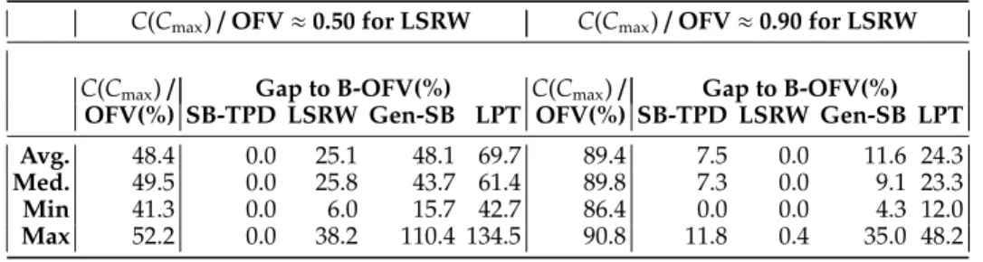
Table 3: Results for the job shop total weighted E/T instances with intermediate inventory holding costs.

πj∼ϵj·U(100,200)% πj∼ϵj·U(200,400)%

f=1.0

B-WT/ Gap to B-OFV(%) B-WT/ Gap to B-OFV(%)

B-OFV(%) SB-TPD LSRW SB-WT Gen-SB ATC B-OFV(%) SB-TPD LSRW SB-WT Gen-SB ATC

Avg. 87.5 10.4 0.1 9.4 43.0 44.9 93.3 9.0 0.3 9.9 41.9 45.0

Med. 87.4 9.8 0.0 9.1 42.6 42.0 93.3 9.4 0.0 8.0 40.3 42.9

Min 83.9 0.0 0.0 0.0 4.1 16.4 91.2 0.0 0.0 0.0 3.8 14.7

Max 90.1 28.3 2.0 26.6 77.8 99.3 95.2 17.4 6.1 25.7 74.4 99.2

f=1.3

B-WT/ Gap to B-OFV(%) B-WT/ Gap to B-OFV(%)

B-OFV(%) SB-TPD LSRW SB-WT Gen-SB ATC B-OFV(%) SB-TPD LSRW SB-WT Gen-SB ATC

Avg. 54.1 12.1 1.0 10.7 70.6 123.0 69.6 14.6 0.5 11.5 80.1 147.4

Med. 54.2 11.9 0.0 10.6 54.6 111.1 70.2 12.3 0.0 10.7 67.3 133.4

πj∼ϵj·U(100,200)% πj∼ϵj·U(200,400)%

Max 73.8 37.2 10.9 30.6 203.7 293.6 85.0 40.8 4.0 38.8 276.6 397.0

f=1.5

B-WT/ Gap to B-OFV(%) B-WT/ Gap to B-OFV(%)

B-OFV(%) SB-TPD LSRW SB-WT Gen-SB ATC B-OFV(%) SB-TPD LSRW SB-WT Gen-SB ATC

Avg. 13.0 2.3 16.2 21.8 57.9 142.2 20.4 7.2 7.3 14.3 78.0 196.2

Med. 9.7 0.0 12.5 16.0 51.2 138.5 16.4 3.4 1.2 9.7 61.0 184.9

Min 0.0 0.0 0.0 0.0 10.0 71.3 0.0 0.0 0.0 0.0 13.3 96.1

Max 40.0 21.2 63.2 70.5 141.2 293.6 56.4 42.5 55.5 63.2 212.1 475.8

f=1.7

B-WT/ Gap to B-OFV(%) B-WT/ Gap to B-OFV(%)

B-OFV(%) SB-TPD LSRW SB-WT Gen-SB ATC B-OFV(%) SB-TPD LSRW SB-WT Gen-SB ATC

Avg. 1.3 0.0 52.7 54.3 51.2 127.2 2.1 0.0 44.9 47.1 59.4 165.5

Med. 0.0 0.0 48.8 55.0 47.4 119.5 0.0 0.0 38.6 51.5 52.7 150.8

Min 0.0 0.0 19.8 17.2 22.8 57.4 0.0 0.0 5.3 6.3 24.1 92.4

Max 12.1 0.0 90.6 99.3 144.4 282.6 21.3 0.0 96.8 92.0 150.3 350.8

f=2.0

B-WT/ Gap to B-OFV(%) B-WT/ Gap to B-OFV(%)

B-OFV(%) SB-TPD LSRW SB-WT Gen-SB ATC B-OFV(%) SB-TPD LSRW SB-WT Gen-SB ATC

Avg. 0.0 0.0 97.6 116.8 55.6 149.7 0.0 0.0 89.3 106.3 51.5 155.1

Med. 0.0 0.0 99.0 110.3 47.8 132.8 0.0 0.0 77.4 103.9 48.3 136.9

Min 0.0 0.0 33.6 68.4 30.9 76.7 0.0 0.0 30.1 45.6 23.0 88.3

Max 0.0 0.0 245.5 240.9 82.6 314.3 0.0 0.0 244.5 190.2 80.2 373.8

For each instance, we calculate the best objective function value (“B-OFV”) obtained over five alternate algorithms, and all gaps in Table3are calculated with respect to the best available solutions. Furthermore, in order to justify our benchmarking strategy against algorithms developed for JS-TWT we compute the minimum total weighted tardiness cost (“B-TWT”) over all algorithms applied to an instance, and we report statistics on the ratio of B-TWT to B-OFV in the first column of Table3. Forf =1.0,1.3, the average of the ratio B-TWT/B-OFV is 90.4% and 61.9%, respectively. Thus, for these instances we expect that the schedules obtained from algorithms designed for JS-TWT perform very well.

For f = 1.0, LSRW is the best contender. SB-TPD performs on a par with SB-WT, and both of these algorithms have an average gap of 9-10% from the best available solution. The fact that the tardiness costs dictate the schedule is also reflected in the gaps obtained by considering tardiness costs only. These figures (not reported here) are close to their counterparts with inventory holding and earliness costs. Both Gen-SB and the ATC dispatch rule have average gaps of more than 40% with respect to the best available solution.

For f = 1.3, LSRW again outperforms the other algorithms. SB-TBD performs slightly worse than SB-WT. The average gap of SB-TPD is on average 12.1% and 14.6% with respect to the best available solution for instances with small and large tardiness costs, respectively. The corresponding figures for SB-WT are 10.7% and 11.5%, respectively. Gen-SB has an average gap of 70.6% and 80.1% with respect to to the best available solution for instances with small and large tardiness costs, respectively. For ATC, these average gaps are at 123.0% and 147.4%, respectively.

For f = 1.5, the average of the ratio B-WT to B-OFV drops to 16.7%. That is, the inventory holding and earliness costs become crucial. In this case, SB-TPD is superior to all other algorithms. For small tardiness costs, the average gaps with respect to the best available solution are 2.3%, 16.2%, and 21.8% for SB-TPD, LSRW, and SB-WT, respectively. The corresponding average gaps for large tardiness costs are obtained as 7.2%, 7.3%, and 14.3%, respectively. The two other algorithms lag by a large margin as for f=1.0 and f=1.3.

For f = 1.7 and f = 2.0, the tardiness costs can almost always be totally eliminated. For these instances, SB-TPD always produces the best schedule. All other algorithms have average gaps of at least 45% with respect to our algorithm.

In SB-TPD, the time until the best solution identified is 782 seconds on average over all instances with no clear trend in solution times as a function of f or the relative magnitude of the unit tardiness costs to the unit earliness costs. However, on average 68% of this time is spent on calculating the single-machine cost functions which requires inverting the optimal basis of the optimal timing problem in the Excel/VB environment. This time can be eliminated totally if the algorithm is implemented in C/C++ using the correspondingCPLEXlibrary which provides direct access to the inverse of the optimal basis. The second main component of the solution time is expended while solving the preemptive relaxation of 1/rj/∑ϵjEj+πjTj as part of the single-machine subproblem and constitutes about 9% of the total

solution time. On the other hand, the time required byCPLEXfor solving the optimal timing problems is only about 4% of the total time on average. Clearly, SB-TPD has great potential to provide excellent solutions in short CPU times. Furthermore, by pursuing the different branches of the search tree on different processors, SB-TPD can be parallelized in a straightforward manner and the solution times may be reduced further.

In general, we expect to obtain high-quality solutions early during SB-TPD if the subproblem definition is appropriate and the associated solution procedure is effective. In AppendixC, we present a detailed analysis of the rate at which good incumbent solution are found and improved. In general, our procedure finds very good solutions (and often the best solutions found) early during the heuristic run.

4.2 Job Shop Total Weighted Completion Time Problem with Intermediate Inventory Holding Costs

4.2.1 Benchmarking Against Heuristics The instances in the previous section are converted into total weighted completion time instances by setting the due dates to zero. The same set of algorithms are applied to the resulting 44 instances, except that the ATC dispatch rule is substituted by the Weighted Shortest Processing Time (WSPT) dispatch rule which is more appropriate for weighed completion time problems. Note that the WSPT rule implemented in LEKIN⃝R- Flexible Job-Shop Scheduling System

(2002) computes the priority of an operationoij by taking into account the total remaining processing

time of jobj. The results are presented in Table4.

Table 4: Results for the job shop total weighted completion time instances with intermediate inventory holding costs.

πj∼ϵj·U(100,200)% πj∼ϵj·U(200,400)%

B-WC/ Gap to B-OFV(%) B-WC/ Gap to B-OFV(%)

B-OFV(%) SB-TPD LSRW SB-WT Gen-SB WSPT B-OFV(%) SB-TPD LSRW SB-WT Gen-SB WSPT

Avg. 96.7 2.0 0.4 1.8 10.8 10.7 98.3 1.8 0.4 1.8 9.9 10.1

Med. 96.6 1.9 0.0 1.5 9.8 10.2 98.3 1.8 0.0 1.5 8.1 9.5

Min 95.6 0.0 0.0 0.0 2.3 3.4 97.7 0.0 0.0 0.0 3.2 3.2

Max 97.9 6.7 3.3 5.6 24.6 21.7 98.9 3.9 2.2 6.6 23.7 20.8

As in Section 4.1.2, we calculate the best objective function value (“B-OFV”) obtained over five alternate algorithms for each instance, and the gaps reported in Table4are based on the best available solutions. Statistics on the ratio of the minimum total weighted completion time cost (“B-WC”) over all algorithms to B-OFV are provided in the first column of Table4and justify our benchmarking strategy. For all instances, the ratio B-WC/B-OFV stands above 95%. The job shop total weighted completion time problem with inventory holding costs appears to be easier in practice compared to its counterpart with tardiness costs. SB-WT and SB-TPD perform on a par, while LSRW exhibits slightly better gaps. For small unit completion time (tardiness) costs, the average gaps with respect to the best available solution are 2.0%, 0.4%, and 1.8% for SB-TPD, LSRW, and SB-WT, respectively. Doubling the unit completion time costs leads to the average solution gaps 1.8%, 0.4%, and 1.8% for these three algorithms, respectively. The two other algorithms Gen-SB and WSPT are on average about 10% offthe best available solution.

For the total weighted completion time instances with inventory holding costs, SB-TPD takes an average of 817 seconds until the best solution is identified with a similar composition to that in Section