Time-Optimal Online Trajectory Generator for Robotic Manipulators
Francisco Ramos, Mohanarajah Gajamohan, Nico Huebel and Raffaello D’Andrea
Abstract— This work presents a trajectory generator for time-optimal maneuvering of a robotic manipulator in joint-space. This generator allows to adapt these maneuvers depend-ing on external events received by the robot (e.g. from sensors or human input). Closed-form equations for these trajectories are provided, resulting on a computationally light algorithm which can update the trajectory at any time taking into account the current state of the robot and the final desired state.
The contribution of this paper is an implementation of the al-gorithm which is available under LGPL for the use of the com-munity. This implementation has been designed to work with KUKA Fast Research Interface (FRI). As a test-bed, a KUKA Light Weight Robot with seven degrees-of-freedom was used, and the experimental results are summarized in this article. The source code of the trajectory generator is available athttps: //github.com/IDSCETHZurich/trajectory-generator
I. INTRODUCTION
Trajectory design is a topic of capital importance in industrial robotics and, as such, it has been developing since first robots were ever released and there are chapters devoted to the generation of trajectories in almost every textbook on robotics [1]. Their importance is tightly related to productivity in assembly chains (the faster the trajectories, the higher the production), but also to the durability of the robot elements, such as motors, or the avoidance of vibrations at the tip of the arm.
In this paper we deal with online generation of time-optimal trajectories. While traditional approaches design the trajectory offline [2], [3] and execute it afterwards ignoring any new information regarding the environment, the online trajectory generation approach attempts to generate trajec-tories that can react instantaneously to unforeseen external events. This problem is attracting considerable attention lately [4] as robots are beginning to operate outside of the factories where they performed repetitive tasks in structured environments. New applications demand from them the abil-ity to interact with their environments, or at least, react to events that happen in them [5].
Therefore, the trajectories have to be modified during execution time, depending on external factors such as sensor measurements or human commands. In [6], [7], Kr¨oger and Wahl show a general solution to this problem. Every time instant they calculate the next reference position based on the current state of the robot and the final desired state.
F. Ramos is with the School of Industrial Engineering, University of Castilla-La Mancha, 13071 Ciudad Real, Spain
francisco.ramos@uclm.es
G. Mohanarajah, N. Huebel and R. D’Andrea are with the Institute for Dynamic Systems and Control, ETH Zurich, 8092 Zurich, Switzerland
{gajan,nhuebel,rdandrea}@ethz.ch
While their work proposes a very general solution, it also requires a not-negligible amount of calculations at every time instant, and the classification stage grows exponentially with the number of derivatives accounted for in the robot state model. In this work we take a different approach that saves computation time. We only recalculate the trajectories, whenever a new event arrives to the trajectory generator, while we can get the position from evaluating a polynomial at every time step. Furthermore, the classification depends only on two parameters that can be calculated in a straightforward manner.
The article is structured as follows. First, Section II intro-duces the problem framework and the notation and provides a general structure for the solution. Then, the velocity profiles of a specific case are calculated in Section III, and Section IV states a procedure for synchronizing the trajectories of the joints in a maneuver. Finally, the experimental setup is described and the experimental results are analyzed in Section V before conclusions are drawn.
II. TIME-OPTIMAL TRAJECTORIES
We aim to find a family of trajectories that solve the problem of moving a robot manipulator withmjoints from an initial state to a final state in a time-optimal fashion. We define the state of the system at instanttas
X(t) = 1x(t),2x(t), ...,mx(t), (1) where
lx(t) = lp(t), lv(t)
(2) represents the state of a single jointlat timet, which consists of position,lp(t)and velocity,lv(t), of the joint. In addition, we define the acceleration of joint l, la(t), as the control input to the system.
These variables are bounded by the following joint space and control input limits
la
m≤la(t)≤laM lv
m≤lv(t)≤lvM lp
m≤lp(t)≤lpM
∀t∈(0, tf). (3)
We only consider the kinematic model of the system in this work. Hence, the maneuver can be decoupled for each joint and calculated separately, so we will drop the l index and assume that we are calculating the time-optimal maneuver for a generic joint. We also assume that the robot cannot collide with itself as long as we are moving within the joint space, which is a common design requirement for industrial manipulators [8].
A. Problem solution
The time optimal problem for each joint can be stated as:
Find the optimal inputa∗(t)that minimizes
Z tf
0
dt
subject tothe following system equations
v(t) = dp(t)
dt a(t) = dv(t)
dt (4)
the initial and final constraints
xi=x(0) = (pi, vi)
xf =x(tf) = (pf, vf),
(5) and the state and input constraints given by equation (3).
This is a well-known control problem that can be solved using Pontryagin’s Minimum Principle [9] and the direct adjoining approach to handle the constraints. Then, from corollary 5.2 in [10], it can be demonstrated that the the control input that provides a time-optimal solution is a piece-wise bang-zero-bang profile. The state and control profiles are given by the following polynomial equations
pj(t) = 12aj0(t−Tj)2+vj0(t−Tj) +pj0 (6)
vj(t) = aj0(t−Tj) +vj0 (7)
aj(t) = aj0, (8)
where pj0, vj0 and aj0 are the initial values of the states
and the control input in the j-th piece, and Tj is the initial time of the piece. Assuming that actuator limits are identical in both positive and negative directions, the constraints from (3) become
|a(t)| ≤aM, |v(t)| ≤vM, |p(t)| ≤pM, ∀t∈(0, tf),
(9)
B. Note on the final velocities
The use of final velocities different from zero raises two additional problems, as not all states that satisfy (9) can be reached without implying a previous or posterior violation of those same constraints:
• Non-decelerable final state: these states are reachable from within the feasible region of the state-space, but they will conflict with the position constraints after the end of the trajectory. Assuming that our final velocity isvf, the minimum distance covered when decelerating to zero would be
∆pdec=
vf· |vf|
2aM
. (10)
As the position at rest must be within the limits given by (9), it follows that
|pf+ ∆pdec| ≤pM, (11)
or we would not be able to stop the movement without violating the position constraints.
• Non-reachable final state: these states are within the feasible region of the phase space defined by (9), but cannot be reached without leaving that feasible region previously. That is, the distance needed to accelerate to vf from 0 is given by Eq. (10), with |∆pacc| =
|∆pdec|. Therefore, for the final state to be reachable,
the position, at rest, from where we approach it must fulfil
|pf−∆pacc| ≤pM, (12)
vf
pf + Δpdec pf - Δpacc
vf
pf
pf
pi
pi
vi
vi
Fig. 1: Outline of non-decelerable and non-reachable final states due to final velocities
From conditions (11) and (12) the following additional feasibility condition can be derived for the desired final state of the trajectory can be joined in a single statement as
max (|pf+ ∆pdec|,|pf−∆pacc|)≤pM. (13) III. VELOCITY PROFILES
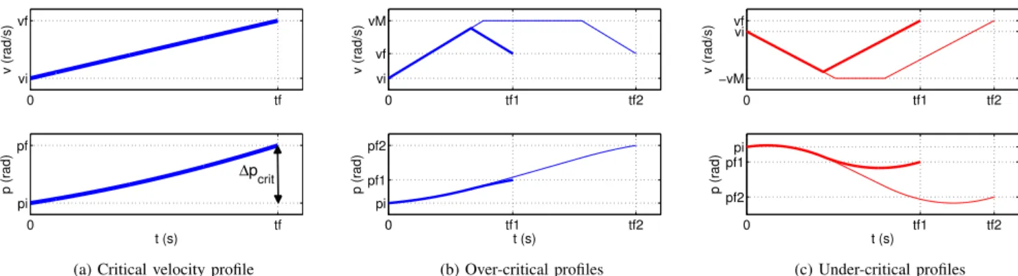
Depending on the values of the initial state and the final desired state, we will obtain different trajectory shapes. In this work we will use the velocity profile to classify the trajectories into three cases: critical, over-critical and under-critical. For simplification, both initial and final velocities of the trajectory will be considered positive in the analysis, but the results extend to any pair of velocities within the limits given by (9) and (13).
A. Critical profile
We define a critical profile that consists of a linear velocity profile between initial and final velocities at a constant accelerationaM (see Fig. 2a). This profile defines a threshold between accelerating and decelerating from the initial state. Let us define ∆p =pf −pi and ∆v =vf−vi. Then the duration of this profile is
tcritf =s˜v∆v
aM
(14) and the distance covered during the maneuver is given by
∆pcrit= ¯v·tcritf = ˜
sv
v2
f−v
2
i
2aM
, (15)
where˜sv=sign(∆v).
In the case ∆p = ∆pcrit, no further calculations are needed, and the piecewise polynomial solution consists of a single piece
a1(t) = ˜svaM v1(t) = ˜svaMt+vi
p1(t) = 12s˜vaMt2+vit+pi
t∈
0, tcritf
0 tf pi
pf
t (s)
p (rad)
0 tf
vi vf
v (rad/s)
∆pcrit
(a) Critical velocity profile
0 tf1 tf2
pi pf1 pf2
t (s)
p (rad)
0 tf1 tf2
vi vf vM
v (rad/s)
(b) Over-critical profiles
0 tf1 tf2
pf2 pf1 pi
t (s)
p (rad)
0 tf1 tf2
−vM vi vf
v (rad/s)
(c) Under-critical profiles
Fig. 2: Velocity profiles classification depending on the comparison between∆pand∆pcrit.
The duration of a critical profile is the minimum time that a trajectory with such values of initial and final velocity can take. When the distance to cover is longer or even shorter than∆pcrit, the duration of the trajectory will be longer than the critical, as we will discuss in the following subsections.
B. Over-critical profile (∆p >∆pcrit)
In this case, as the distance to cover is longer than the criti-cal, the maneuver will require more time to be accomplished. Let us first assume that the velocity profile is triangular and, hence, is divided into two parts: 1) acceleration, and 2) deceleration (see Fig. 2b). The peak velocity achieved during the motion is given by
vpo= r
∆p·aM +
1 2
v2
f+vi2
. (17)
The triangular profile will be feasible if vpo < vM. Oth-erwise, the system will follow a trapezoidal profile with three parts: 1) acceleration, 2) constant speed atvM, and 3) deceleration (see Fig. 2b). Equations for both profiles will be treated in Section III-D.
C. Under-critical profile (∆p <∆pcrit)
This case requests a shorter position movement and, therefore, we may be inclined to think that its duration should be also shorter. However, the final velocity restriction causes the joint first to move backwards to reach point pcrit
i =pf−∆pcritat velocityvi, and then perform a critical maneuver in order to achieve the final desired state. Hence, the total trajectory will also be longer than the critical.
However, the profile shape is similar to that of the over-critical profile. Again, we determine the profile to be tri-angular or trapezoidal (see Fig. (2c))depending on the peak velocity, which, in this case, is given by
vpu=− r
1 2
v2
f+v2i
−∆p·aM. (18)
D. Equations of a generic non-critical profile
Under and over-critical profiles can be expressed in a single formulation by defining the sign of the trajectory as
˜
s=sign ∆p−∆pcrit (19)
and the peak speed (assuming a triangular profile) as vp =
r
1 2
v2
f+v
2
i
+ ˜s·∆p·aM. (20) Equation (19) also gives the sign of the initial acceleration of the profile, while (20) provides a criterion to classify the profile.
1) Triangular profile (vp ≤ vM): This is a bang-bang acceleration profile with two parts:
• First piece, t ∈ (0, T1), from initial velocity to peak
velocity
a1(t) = ˜saM v1(t) = ˜saMt+vi
p1(t) = 12sa˜ Mt2+vit+pi.
(21)
• Second piece, t∈(T1, tf], from peak velocity to final velocity
a2(t) = −sa˜ M
v2(t) = −sa˜ M(t−T1) + ˜svp
p2(t) = −21˜saM(t−T1)2+ ˜svp(t−T1) +p1(T1).
(22)
• Switching times: to completely define this trajectory we only need to calculateT1 andtf, which are given by
T1 =
˜
svp−vi
˜
saM tf = T1+
vf−˜svp
−sa˜ M
.
(23)
2) Trapezoidal profile (vp > vM): In this case, the distance to cover is long enough such that the velocity reaches its maximum admissible value. Hence, the profile will have three parts:
• First piece,t∈[0, T1], from initial to maximum velocity
a1(t) = ˜saM v1(t) = ˜saMt+vi
p1(t) = 12sa˜ Mt2+vit+pi.
(24)
• Second piece t∈(T1, T2], motion at constant velocity
˜
svM
a2(t) = 0
v2(t) = sv˜ M
p2(t) = sv˜ M(t−T1) +p1(T1).
• Third piecet∈(T2, tf], from maximum to final velocity a3(t) = −sa˜ M
v3(t) = −sa˜ M(t−T2) + ˜svM
p3(t) = −21˜saM(t−T2)2+ ˜svM(t−T2) +p2(T2).
(26)
• Switching times:T1,T2 andtf can be calculated from T1 =
˜
svM−vi
˜
saM T2 =
1
vM "
v2
f+vi2−2˜svMvi
2aM
+ ˜s∆p #
tf = T2+
vf−sv˜ M
˜
saM .
(27)
This is a compact, straightforward formulation for the event-driven online trajectory generation problem that functions for any set of initial and final conditions (pi,pf,vi andvf) satisfying (9) and (13).
IV. TRAJECTORY SYNCHRONIZATION Most maneuvers of the robot will have different durations for each joint trajectory and the shorter ones will already have finished their motions while the longer ones are still moving. Hence, there is no need for the shorter trajectories to be performed in a time-optimal way and they could use some of this extra time to make their profiles less demanding for the actuators, hence extending their lifetime. This procedure is what we will define as synchronization: a maneuver is synchronized if all joints arrive at their target positions at the same time instant.
To achieve this, new synchronized trajectory profiles that take the final time as an input have been developed.
The synchronization procedure consists of three steps
• Calculate the minimum time of every joint profile and choose the synchronizing time as the maximum of them tsyncf = maxltf, l= 1, ..., m. (28) • Determine the shape of synchronized velocity profile
for every joint.
• Calculate the parameters and coefficients of the profiles. The first step is straightforward from the equations given in previous Section, and hence it will not be further detailed. However, the shape of the synchronized profile is a rich problem in terms of the choice of the design parameters. As we now relax the optimal-time requirement and only fix the final time of the trajectory, we have a new degree of freedom in the equations, which could be used in a number of ways (i.e. reducing the maximum demanded acceleration). In this paper we approach the problem by minimizing the value of the velocity at the constant velocity piece of each individual joint,vc, such that all joints reach the final position at time tsyncf while keeping the acceleration value at its maximum, aM, during the acceleration and deceleration pieces. However, the duration of these pieces will be reduced. With these constraints in mind, the different synchronized profiles have been outlined in Fig. 3. For the trajectory
0 0
time−optimal trapezoidal limit double ramp vM
vi
tfopt tflim
Fig. 3: Different shapes of the velocity profiles depending on the synchronization time
synchronization, we will assume that the final velocity is zero.
We can see that there is a limit case, which separates trapezoidal from double ramp profiles, when vc = vi. The duration of this limit case has to be calculated separately for each joint, yielding
tlimf = ∆p
vi
+˜s·vi 2aM
. (29)
Then, comparing this value withtsyncf , we can determine the shape of the trajectory: trapezoidal profile iftsyncf < tlim
f or
double-ramp profile otherwise.
The expression ofvc will differ for each profile • Trapezoidal profile:
vc=
1 2
b−
q
b2−4˜s·a
M∆p−2v2i
, (30)
whereb=aMtsyncf + ˜s·vi. • Double-ramp profile:
vc =
˜
s·∆p− v
2
i
2aM tsyncf − vi
˜
s·aM
. (31)
The equations of the synchronized trajectory will be very similar to those of the trapezoidal profile, only substituting vM byvcand including a new signs˜t=sign(tlimf −t
sync f ), that makes a general formulation valid for both trapezoidal and double-ramp profiles, yielding
• First piece,t∈(0, T1): initial to constant velocity.
a1(t) = ˜s˜staM v1(t) = ˜s˜staMt+vi
p1(t) = 12s˜s˜taMt2+vit+pi.
(32)
• Second piece, t∈(T1, T2): constant velocity at sv˜ M. a2(t) = 0
v2(t) = ˜svc
p2(t) = ˜svc(t−T1) +p1(T1).
(33)
• Third piece,t∈(T2, t
sync
f ): fromsv˜ M to final velocity. a3(t) = −sa˜ M
v3(t) = −sa˜ M(t−T2) + ˜svc
p3(t) = −21˜saM(t−T2)2+ ˜svc(t−T2) +p2(T2).
Obviously, the switching times will be different for this profile than those of the optimal trajectory
T1 =
˜
svc−vi
˜
ss˜taM T2 = tsyncf −
vc aM
.
(35)
V. EXPERIMENTS
To show the performance of our trajectory generator, experimental results will be presented in this section.
A. Experimental Setup
The trajectory generator has been tested on a KUKA Light Weight Robot (LWR) with seven degrees of freedom. For our software setup we were using the Robot Operating System (ROS) [11] and the Open Robot Control Software (OROCOS) [12]. We were using a ROS node to generate random joint positions at a rate of 1 s. These positions were sent to our trajectory generator OROCOS component. To couple our trajectory generator with the KUKA FRI the OROCOS LWR FRI component was used. More information on this component can be found athttp://www.ros.org/ wiki/lwr_fri.
Trajectory
Generator LWR_FRI
Next Final Joint Position
[1 s]
Commanded Joint Position [20 ms]
UDP Packets [1 ms] Measured
Robot State [1 ms]
ROS OROCOS KRC
Fig. 4: Experimental setup
Whenever the trajectory generator component receives a new final desired position, it gets the current state of the robot from the LWR FRI component and calculates the new trajectory to reach the new final position taking into account the current position and velocity of the robot. After calculating the trajectory polynomials, they can be evaluated at the current time whenever the FRI is requesting a new position. This event-based architecture was chosen to avoid synchronization problems between the FRI running on the KUKA Robot Controller (KRC) and the OROCOS and ROS components running on the remote computer.
B. Source Code of the Trajectory Generator
The trajectory generator is available at https://github. com/IDSCETHZurich/trajectory-generator, under LGPL. This repository contains all nodes and components required to run the setup described above (except for the FRI, which must be provided by KUKA). If a real KUKA LWR is not available or the behavior of newly developed code using the trajectory generator should first be tested without endangering the real robot, a script file offers to reroute the output to the ROS visualization environment RVIZ (http: //www.ros.org/wiki/rviz). Please be aware that this is only a visualization of the kinematics, which does not take into account the dynamics of the robot. README files,
0 0.5 1 1.5
−2 0 2
angles(rad)
t(s)
0 0.5 1 1.5
−2 0 2
veloticies(rad/s)
(a) Time-optimal
0 0.5 1 1.5
−2 0 2
angles(rad)
t(s)
0 0.5 1 1.5
−2 0 2
veloticies(rad/s)
(b) Synchronized
Fig. 5: Single maneuver of the robot
explaining the content, setup, and use of each package, are provided as well. If you should encounter problems or have questions, feel free to contact the authors.
C. Results
Figure 5 shows a single maneuver performed by the robot using time optimal trajectories for all joints (Fig. 5a) and using synchronized trajectories (Fig. 5b). Notice that when we use the synchronization procedure, the acceleration periods of each joint (except for the longest time-optimal trajectory) are reduced with respect to the set of original time-optimal profiles, while the overall maneuver duration remains the same.
The most interesting feature of this work is the ability to interrupt trajectories depending on unforeseen events (human or sensor driven). In Fig. 6, two excerpts of the profiles generated during longer runs of the robot are shown. Fig. 6a shows the joint velocity profiles when the time-optimal trajectories are used in the robot, while Fig. 6b gives an example of the velocity profiles when the joint trajectories are synchronized. The position profiles are smooth during the whole sequence of maneuvers even when they are interrupted by new events. This shows the advantage of considering the current state in the updating of the trajectories, which is one of the main goals of this work.
Maneuvers are clearly more abrupt when they are not synchronized, and there are also more rest periods for the joints, while the synchronized motions are smoother but there are no rests in the whole sequence of maneuvers. Velocities are also more steady in the synchronized maneuvers, while they are almost constantly changing in the time-optimal case, showing that the use of acceleration (and hence, motor torques) is reduced with synchronization.
VI. CONCLUSIONS
In this paper, a trajectory generator for robotic arms that takes into account the kinematics of the arm has been studied. The trajectory profiles have been calculated in a time-optimal manner, obtaining a compact, computationally light formulation which works for any set of initial and final states within the robot limits. Due to this, the trajectory generator can be event-driven and dynamically update the current trajectory of each joint whenever a new desired final state arrives. This is a convenient feature of a trajectory
10 11 12 13 14 15 16 17 18 −1
0 1
FRI POSITIONS Robot Side | Solid:commanded | Dashed:measured
t(s)
joint angles
(rad)
10 11 12 13 14 15 16 17 18
−1 0 1
FRI VELOCITIES Robot Side | Solid:commanded | Dashed:measured
joint velocities
(rad/s)
(a) Non-synchronized maneuvers.
10 11 12 13 14 15 16 17 18
−1 0 1
FRI POSITIONS Robot Side | Dashed:commanded | Solid:measured
t(s)
joint angles
(rad)
10 11 12 13 14 15 16 17 18
−1 0 1
FRI VELOCITIES Robot Side | Dashed:commanded | Solid:measured
joint velocities
(rad/s)
(b) Synchronized maneuvers.
Fig. 6: Continuous motion of each joint of the KUKA LWR. New targets state every second.
generator, as there are a number of applications in which we would like to modify the original trajectory based on sensor information, especially for service robotics, where the robot must dynamically react to changes in the environment.
The trajectory generator has been implemented to work with some of the most used software packages in the robotics community (ROS, OROCOS), and is available under LGPL in a public git repository at https://github. com/IDSCETHZurich/trajectory-generator. Even if no physical robot is available, the trajectory generator opera-tion and performance can be checked in simulaopera-tion following the instructions found in the code repository.
The same approach taken in this paper will be extended in future works to more general trajectories that include synchronization with non-zero final velocities, and higher order control inputs (jerk, snap).
VII. ACKNOWLEDGMENTS
This research was funded by the European Union Seventh Framework Programme FP7/2007-2013 under grant agree-ment no. 248942 RoboEarth.
REFERENCES
[1] B. Siciliano, L. Sciavicco, L. Villani, and G. Oriolo,Robotics. Mod-elling, Planning and Control. Springer, 2009.
[2] K. G. Shin and N. D. McKay, “Minimum-time control of robotic manipulators with geometric path constraints,” Automatic Control, IEEE Transactions on, vol. 30, no. 6, pp. 531 – 541, jun 1985.
[3] H. Geering, L. Guzzella, S. Hepner, and C. Onder, “Time-optimal motions of robots in assembly tasks,”Automatic Control, IEEE Trans-actions on, vol. 31, no. 6, pp. 512 – 518, jun 1986.
[4] J. Kim, S.-R. Kim, S.-J. Kim, and D.-H. Kim, “A practical approach for minimum-time trajectory planning for industrial robots,”Industrial Robot: An International Journal, vol. 37, no. 1, pp. 51–61, 2010. [5] J. Lloyd and V. Hayward, “Trajectory generation for sensor-driven and
time-varying tasks,”The International Journal of Robotics Research, vol. 12, no. 4, pp. 380–393, 1993.
[6] T. Kr¨oger, A. Tomiczek, and F. M. Wahl, “Towards on-line trajectory computation,” inProc. of the IEEE/RSJ International Conference on Intelligent Robots and Systems, Beijing, China, oct 2006, pp. 736–741. [7] T. Kr¨oger and F. M. Wahl, “On-line trajectory generation: Basic concepts for instantaneous reactions to unforeseen events,” IEEE Trans. on Robotics, vol. 26, no. 1, pp. 94–111, feb 2010.
[8] M. Shimizu, H. Kakuya, W. . Yoon, K. Kitagaki, and K. Kosuge, “Analytical inverse kinematic computation for 7-dof redundant manip-ulators with joint limits and its application to redundancy resolution,”
IEEE Transactions on Robotics, vol. 24, no. 5, pp. 1131–1142, 2008. [9] D. P. Bertsekas,Dynamic Programming and Optimal Control. Athena
Scientific, 2007.
[10] H. Maurer, “Optimal-control problems with bounded state variables and control appearing linearly,”SIAM Journal on Control and Opti-mization, vol. 15, no. 3, pp. 345–362, 1977.
[11] Willow Garage, “Robot Operating System (ROS),” 2009, [Last visited 2011].
[12] H. Bruyninckx, “Open Robot COntrol Software,” 2001, [Last visited 2011].