ISSN: 1311-1728 (printed version); ISSN: 1314-8060 (on-line version) doi:http://dx.doi.org/10.12732/ijam.v31i5.9
SINGLE MACHINE SLACK DUE-WINDOW SCHEDULING WITH LINEAR RESOURCE ALLOCATION AND
POSITION-DEPENDENT PROCESSING TIMES Bo Cheng1§, Ling Cheng2
1Department of Applied Mathematics School of Finance
Guangdong University of Foreign Studies Guangzhou, 510420, CHINA
2School of Electrical and Information Engineering University of the Witwatersrand
Private Bag 3, Wits. 2050, Johannesburg, SOUTH AFRICA
Abstract: In this paper, we investigate single machine scheduling with linear resource allocation and position-dependent processing times based on the slack due-window method. The objective is to minimize the total cost caused by the due-window location, the due-window size, the resource consumption, the makespan and the earliness and tardiness with respect to a slack due-window. We provide a polynomial-time algorithm to solve the problem.
AMS Subject Classification: 90B35
Key Words: resource allocation, due-window, machine scheduling, resource consumption model
1. Introduction
In the classical scheduling theory, job processing times are considered as con-stants. However, in the last decade we have witnessed a steadily growing interest on solving scheduling problems with changeable job processing times. There is a practical merit of considering changeable job processing times. In practice, the processing time of a job can be dependent on the position scheduled, and
the phenomenon that the actual processing time of a job can be reduced due to an additional resource allocated to the job has been noted. It prompts the stud-ies on a variety of single machine scheduling models and assignment problems taking into account the effects of resource allocation and position-dependent processing times.
Conventionally, there are a few due-window methods, for example, common due-window and slack due-window. In this paper, we investigate the single machine scheduling and slack due-window assignment problem with resource allocation and position-dependent processing times. To our best knowledge, this problem has not been studied in literatures. In a relevant work, [1] investigated a similar model but with position-independent processing times. In this paper, we generalize this model by assuming that the processing times are position-dependent.
The rest of this paper is organized as follows. The problem under study is illustrated in Section 2. The optimal (polynomial-time) solution is presented in Section 3. A numerical example to demonstrate the polynomial-time solution is given in Section 4. The research is concluded and future study is foreseen in the last section.
2. Model Formulation
In the models of this paper, n independent and non-preemptive jobs J1, J2,
. . . ,Jn are scheduled on a single machine. All the jobs can be arranged at time zero. Let ajr and pjr be the normal and the actual position-dependent processing times of job Jj when it is arranged in the rth position. The actual and the maximum-available resource allocated to job Jj are denoted by uj and ¯uj, respectively. For the linear resource consumption model, the actual processing time of job Jj is determined by
pjr=ajr−cjuj, (1)
wherecj is the positive compression rate of job Jj, 0≤uj ≤u¯j and pjr≥0. The due-window of job Jj is determined by a pair of non-negative real numbers [dj, d′j] such that dj ≤ d′j, where dj and d′j are the beginning and ending times of the due-window respectively. For the slack due-window method,
dj andd′j are decided by
dj =pjr+q, (2)
and
whereq′ > q are two job-independent constants.
Then the due-window sizeDj =dj −d′j =q′−q, for j= 1, . . . , n, is equal for all the jobs. Let D=Dj.
For a given schedule π, Cj denotes the completion time of job Jj, Ej = max{0, dj −Cj} is the earliness value of job Jj, and Tj = max{0, Cj −d′j} is the tardiness value of job Jj. The makespan Cmax = max{Cj|j = 1,2, . . . , n} is the completion time of all jobs. HereCmax is the completion time of the last job scheduled in then’th position.
To this end, we can create the following total cost function
Z =
n X
t=1
(αEt+βTt+γdt+δD) +η n X
t=1
Gtut+θCmax, (4)
which takes into account (i) earliness Ej, (ii) tardiness Tj, (iii) starting time of the due-window dj, (iv) due-window size D, (v) resource consumption uj and (vi) makespan Cmax. We further define α > 0, β > 0, γ > 0 and δ > 0 representing the earliness, tardiness, due-window starting time and due-window size costs per unit time respectively. For the resource consumption cost, Gt is defined as the per unit resource cost for jobJt. Hereη ≥0 and θ≥0 are two constant weights which are specified by the decision-maker.
With the three-field notation of [2], the problem under study is expressed as 1|SLKW, pjr =ajr−cjuj |Pnt=1(αEt+βTt+γdt+δD)+ηPnt=1Gtut+θCmax, whereSLKW in the second field denotes the slack due-window method.
3. Optimal Solution Algorithm
In this section we present some properties for a schedule.The proofs of the fol-lowing lemmas are similar to those in [3], [4], [5] and [6]. We use a conventional notation [r] to indicate the index of a job which is allocated at therth position.
Lemma 1. IfC[r]≥d′[r] holds, thenC[r+1]≥d′[r+1].
Lemma 2. IfC[r]≤d[r] holds, thenC[r−1]≤d[r−1].
Consider a job sequence π and a resource allocation way u = (u1, u2, . . . ,
un). Suppose C[s] ≤ q ≤ C[s+1] and C[t] ≤ q′ ≤ C[t+1]. Then the total cost
Z is a linear function ofq and q′, and hence an optimum is obtained either at
Lemma 3. (i) For any given resource allocation u and job sequence π, there exists an optimal scheduling such thatq andq′ coincide with the comple-tion times of thek-th andl-th jobs (l≥k) in the sequence.
(ii) An optimal scheduling begins at time zero and has no idle time between consecutive jobs.
For a numbera,⌊a⌋ denotes the largest integer less than or equal to a.
Lemma 4. k=jn(δ−γ)α kand l=jn(β−δ)β k.
With Lemma 4, the values of kand l can be obtained. In the following we assume k≤l and refer to [7] for the other cases.
For the objective function, we have
Z =
n X
r=1
(αE[r]+βT[r]+γd[r]+δD) +η
n X
t=1
Gtut+θCmax
= n X
r=1
wrpjr+η n X
t=1
Gtut,
(5)
where
wr=
αr+γ(n+ 1) +θ, 1≤r ≤k, γ+nδ+θ, k < r ≤l, β(n−r) +γ+θ l < r ≤n.
(6)
Since pjr=ajr−cjuj, we have
Z =
n X
r=1
wrajr+ n X
r=1
(ηGj−wrcj)uj, (7)
wherej = [r].
Due to the fact thatpjr≥0, we have uj ≤ acjrj . Setu′j = min{uj,acjrj }, and hence we haveuj ≤u′j.
Note that the optimal resource allocation for jobJj depends on the sign of
ηGj −wrcj. Letu∗j be the optimal resource allocation for job Jj. Then
u∗j =
u′j, if ηGj −wrcj <0,
uj ∈[0, u′j], if ηGj −wrcj = 0, 0, if ηGj −wrcj >0.
(8)
χjr= (
wrajr, if ηGj−wrcj ≥0,
wrajr+ (ηGj −wrcj)u′j, if ηGj−wrcj <0,
(9)
and
zjr= (
1 if job Jj is arranged in therth position
0 otherwise. (10)
To minimize the problem 1 | SLKW, pjr = ajr −cjuj | Pnj=1(αEj +βTj +
γdj +δD) +ηPnj=1Gjuj +θCmax is equivalent to minimizing the following Assignment Problem, which can be solved in time complexityO(n3),
min n X j=1 n X r=1
χjrzjr
s.t. Pn
j=1zjr = 1, r = 1,2, . . . , n, Pn
r=1zjr= 1, j = 1,2, . . . , n,
zjr= 0 or 1, j, r = 1,2, . . . , n.
(11)
Algorithm 1. Solution algorithm for the problem 1|SLKW, pjr=ajr−
cjuj |Pnt=1(αEt+βTt+γdt+δD) +ηPnt=1Gtut+θCmax.
1 SET k=j n(δ−γ)α k, l=j n(β−δ)β k.
2 FOR each position r = 1,2, . . . , n in a schedule
3 DETERMINE the positional weight wr
4 END FOR
5 FOR each job j= 1,2, . . . , n
6 FOR each position r= 1,2, . . . , n in a schedule
7 DETERMINE the value χjr according to (9)
8 END FOR
9 END FOR
10 DETERMINE the global optimal schedule of the assignment problem
described in (11) and its total cost
Theorem 1. Algorithm 1 solves the problem1|SLKW, pjr=ajr−cjuj | Pn
t=1(αEt+βTt+γdt+δD) +ηPnt=1Gtut+θCmax inO(n3) time.
Proof. The correction of Algorithm 1 is guaranteed by Lemmas 4 and
complexity of Step 10 is O(n3). Hence, the time complexity for solving the 1|SLKW, pjr =ajr−cjuj |Pnt=1(αEt+βTt+γdt+δD)+ηPnt=1Gtut+θCmax
problem isO(n3).
Remark. Theorem 3.3 in [1] can be regarded as a special case of Theorem 1.
4. Numerical Example
In this section, Algorithm 1 for the linear resource model presented in Section 3 is demonstrated by the following example.
Example 1. There are n = 7 jobs. The initial settings of all jobs are illustrated by Table 1 and Table 2.
j 1 2 3 4 5 6 7
cj 3 2 3 4 3 4 2
Gj 34 40 25 38 24 48 42
u 8 7 7 6 6 6 7
Table 1: The settings in Example 1.
ajr r= 1 2 3 4 5 6 7
j = 1 50 30 35 40 55 60 70
2 40 20 45 50 40 70 30
3 35 40 55 50 30 45 22
4 45 52 63 28 41 27 39
5 53 62 74 35 27 39 40
6 30 20 54 62 39 40 50
7 30 50 20 30 40 50 60
Table 2: The ajr settings in Example 1.
The penalties for unit earliness, tardiness, due-window starting time and due-window size are α = 2, β = 18, γ = 4 and δ = 5, respectively. The constant weights are specified by the decision-maker as θ= 0.8 and η= 1.
Solution. By Lemma 4, we have the locations of k = jn(δ−γ)α k = 3 and
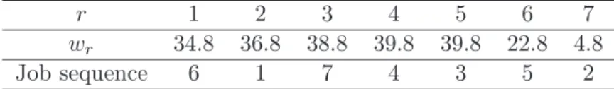
r 1 2 3 4 5 6 7
wr 34.8 36.8 38.8 39.8 39.8 22.8 4.8
Job sequence 6 1 7 4 3 5 2
Table 3: Positional weights in Example 1.
Next, based on (9), we obtain χjr in the following assignment matrix:
1176.80 492.80 698.80 908.80 1505.80 1092.80 336.00 1184.80 500.80 1482.80 1712.80 1314.80 1556.80 144.00 662.20 874.20 1494.20 1329.20 533.20 722.20 105.60 958.80 1258.40 1741.20 387.20 904.60 296.40 187.20 1362.00 1763.20 2316.80 820.60 502.20 622.80 192.00 496.80 240.00 1452.00 1800.40 885.00 652.80 240.00 850.80 1618.80 526.80 930.80 1328.80 1114.80 288.00
(12)
By solving the assignment problem described in (11), we obtain the local opti-mal sequence (6, 1, 7, 4, 3, 5, 2) and the total cost Z = 3203.60.
The global optimal solution for this example includes the following: (i) the job sequence is (6, 1, 7, 4, 3, 5, 2) and the corresponding job starting time and actual processing time are (0, 6, 12, 18, 22, 31, 52) and (6, 6, 6, 4, 9, 21, 30), respectively; (ii) the slack window parameters are q= 18 and q′ = 31; (iii) the optimal resource consumption of each job is (8, 0, 7, 6, 6, 6, 7); (iv) the total cost isZ = 3203.60.
5. Conclusion
References
[1] Y. Yin, T. C. E. Cheng, C.-C. Wu, and S.-R. Cheng, Single-machine due window assignment and scheduling with a common flow allowance and con-trollable job processing time,Journal of the Operational Research Society, 65, No 1 (2014), 1–13.
[2] R. L. Graham, E. L. Lawler, J. K. Lenstra, and A. Kan, Optimization and approximation in deterministic sequencing and scheduling: A survey, Annals of Discrete Mathematics,5 (1979), 287–326.
[3] G. Mosheiov and D. Oron, Job-dependent due-window assignment based on a common flow allowance,Foundations of Computing and Decision Sci-ences,35(2010), 185–195.
[4] B. Mor and G. Mosheiov, Scheduling a maintenance activity and due-window assignment based on common flow allowance,International Jour-nal of Production Economics,135, No 1 (2012), 222–230.
[5] K. Chen, M. Ji, and J. Ge, A note on scheduling a maintenance activity and due-window assignment based on common flow allowance, International Journal of Production Economics,145, No 2 (2013), 645–646.
[6] B. Cheng and L. Cheng, Single machine slack due-window scheduling with linear resource allocation, aging effect, and a deteriorating rate-modifying activity, International Journal of Applied Mathematics, 30, No 5 (2017), 375–386; DOI: 10.12732/ijam.v30i5.2.
[7] M. Ji, J. Ge, K. Chen, and T. Cheng, Single-machine due-window assign-ment and scheduling with resource allocation, aging effect, and a deteri-orating rate-modifying activity, Computers & Industrial Engineering, 66, No 4 (2013), 952–961.
[8] E. Prasetyaningsih, T. Samadhi, and A. Halim, Production and delivery batch scheduling with a common due date and multiple vehicles to mini-mize total cost,IOP Conference Series: Materials Science and Engineer-ing,114, No 1 (2016), 1–10.