BAYESIAN ANALYSIS FOR THE BURR TYPE XII DISTRIBUTION BASED ON RECORD VALUES
M. Nadar, A.S. Papadopoulos
1. INTRODUCTION
The theory and applications of record values is of great importance to scien-tists and engineers and has been studied extensively. For example, predicting the magnitude of an earthquake which has a greater magnitude than the previous o-nes, in a given region, is of importance to seismologists, also predicting the flood level of a river that is greater than the previous ones is of importance to clima-tologists. The theory of record values can be applied to sports records, estimating the strength of materials, etc. Record values are also important to ordinary people and the book “World Guinness Records” chronicles records of sports & games, natural disasters, science & technology, and of all kinds of strange and extreme talents, among others.
Let X X1, 2,... be an infinite sequence of identical independent (iid) random
variables having a common probability density function (pdf) f x( , ) , where θ could be a vector parameter. Intuitively an upper record value, Xj is the
obser-vation which is larger than all previous obserobser-vations. Formally, Xj is an upper
record value if Xj Xi for all i j. The sequence { , 1}Tm m of record times
is defined as follows:
1
1
1
1, with probability 1, and
min{ : >T , m } for 2.
m m j T
T
T j j X X m
Based on the above, the sequence Rm XTm, m1 defines a sequence of upper record values. One can give a similar definition for lower record values.
Let R( ,R R1 2,...,Rm) be a random vector of the upper record values for
intro-duced by Chandler (1952) whereas Feller (1966) gave some examples of record values in gambling. The reader is referred to Arnold et al. (1998), Ahmadi (2000), Feller (1966), Gulati and Padgett (1994), and Nevzorov (2001) for more details on the applications of record values from a statistician’s point of view.
When the underlying distribution is exponential the record values have been studied by Awad and Raqab (2000), they studied four procedures for obtaining prediction intervals for the future s-th record value and by means of computer simulation they compared these procedures. Based on the record values, Ali Mousa (2001) derived three types of estimators, maximum likelihood, minimum variance unbiased and Bayesian estimators for the one parameter Burr type X dis-tribution. Based on record values from the two parameter Pareto distribution, Raqab et al. (2007) obtained maximum likelihood and Bayes estimators for the unknown parameters and point or interval prediction for the future record values. Statistical analysis of record values from the geometric distribution was done by Doostparast and Ahmadi (2006). Furthermore, they derived estimators for the unknown parameter and also considered the problem of predicting the future re-cord values based on past rere-cord values from a non-Bayesian and Bayesian point of view. Based on upper record values, Hendi et al. (2007) obtained Bayes estima-tors, under SEL and LINEX loss functions, for the parameter, reliability function and hazard rate for the Rayleigh distribution. Finally, Ahmadi et al. (2009) studied the prediction of k-records from a general class of distributions under balanced type loss functions.
The purpose of this study is to review and extend some results that have been derived on record values from the two parameter Burr Type XII distribution which was first introduced in the literature by Burr (1942). Its probability density function and cumulative distribution are given below,
1 ( 1)
( ; , ) (1c c) k , , 0
f x c k c k x x x c k (1a)
( , , ) 1 (1 c) k
F x c k x (1b)
In Section 2, we will derive estimators for the parameters c and k, based on record values, review the Bayes estimators that were derived under a SEL func-tion for the parameters by Ahmadi (2000) and also we will derive Bayes estima-tors for c and k under a LINEX loss function. In Section 3, estimates for the fu-ture s-th record value will be derived using non Bayesian and Bayesian ap-proaches. Finally, in Section 4, a numerical example will illustrate the findings of Sections 2 and 3.
2. PARAMETER ESTIMATION
The joint pdf of the first m upper record values according to Arnold et al. (1998) is
1
1 2
1
( ; ) m ( ; ) ( ; ), i m ... m
i
f h r f r r r r
r (2)
where ( , ,... ), ( ; )1 2 ( ; ) ,
1 ( ; )
i
m i
i
f r r r r h r
F r
r and may be a vector, where
is the parameter space. For the Burr Type XII pdf the joint distribution of the first m upper record values reduces to
1
1 2
1
( )
( ; , ) , ... .
(1 ) (1 )
c
m m
i
m
c k c
i
m i
r ck
f c k r r r
r r
r (3)
2.1. MLE Estimation
Suppose we observed the first m upper record values
1 1, ,..., 2 2 m m
R r R r R r from a Burr Type XII, with pdf and cdf given by e-quations (1a) and (1b). Then the joint density function is given by
1
1 m
1
k
( ; , ) , 0, 0; - <r <...<r <
(1 ) (1 )
c
m m m
i
c k c
i
m i
r c
f c k c k
r r
r (4)
Then the log-likelihood function is
1 1
( , ) ln ln ln(1 c) m ( 1)ln m ln(1 c)
m i i
i i
L c k m c m k k r c r r
r (5)
1 1
ln ln
ln 0
1 1
c c
m m
m m i i
i c c
i m i i
kr r r r
m r
c r r
(6)ln(1 mc) 0 m
r
k (7)
The above system is nonlinear, but can be easily solved using numerical tech-niques.
2.2.Bayes Estimation
In this Subsection, we will assume that the parameters and c k of the Burr Type XII distribution are random variables with a joint bivariate density function that was first suggested by Al-Hussaini and Jaheen (1995) and is given by,
1 2
( , ) ( | ) ( )
g c k g k c g c (8)
where
1
1( | ) ( 1) 1 , 1, 0
kc
c
g k c k e
(9)
is the gamma conjugate prior when c is know. This prior was first introduced by Papadopoulos (1978) and was also used later on by Al-Hussaini et al. (1992). The prior of c is
1
2( ) , , 0
( )
c
c
g c e
(10)
which is the gamma(, ) density. With the aid of equations (9) and (10) we ob-tain the bivariate prior of c and k, given as
( , )c k c k exp( (1/c k/ ))
(11)
where 1, , and are positive real numbers.
From (3) and (11), the joint posterior distribution is given by
1
1
1
m+ +1 1
0
exp( (1/ / ))
1 (1 )
( , | )
exp( / ) (m+ +1)
1
ln(1 )
c m
m m
i
c c k
i i m
c m
m i
c
i i c
m
r k
c c k
r r
k c
r c c
r c
r
If the loss function is the well known squared loss function, the Bayes estima-tors for the parameters and c kare the given by the posterior expectations. Ahmadi and Doostparast (2006) derived these estimators and are reproduced be-low, 0 0 1 +2 1 0 1 +1 1 0 ( | ) ( , | )
exp( / ) dc 1
ln(1 )
( 1) .
exp( / ) dc
1 ln(1 ) B c m m i c m
i i c
m
c m
m i
c m
i i c
m
k E k k k c dk dc
r c c
r c
r m
r c c
r c r r r (13) Similarly, 1 1 +1 1 0 1 +1 1 0
exp( / ) dc
1
ln(1 )
xp( / ) dc
1 ln(1 )
e
c m m i c mi i c
m
B c m
m i
c m
i i c
m
r c c
r c
r c
r c c
r c r
(14)Instead of using the well known symmetric SEL function, one can use the asym-metric LINEX loss function which was first proposed by Varian (1975) and is given as
( )
( , ) v ( ) 1
L e v (15)
where θ is a univariate parameter and v0. The parameter v is known and gives the degree of asymmetry. If v0 and the errors are positive, the LINEX loss function is almost exponential and for negative errors almost linear, in this situation overestimation is a more serious problem than underestimation. If
0,
v underestimation is more important than overestimation.
Let M|r( )t E|r(et) be the moment generating function of the Bayes
predictive density function of given .r It can be easily verified that the value of ( ) that minimizes E|r( ( , ( ))L in equation (15) is
*
|
1
( ) lnM ( ),v
v
( , )|
0 0
( vk| ) vk ( , | )
k c
E e e k c dc dk
r r r (16)
For the parameter k the LINEX estimator is
1 +1 1 0 1 +1 1 0
exp( / )
dc 1
ln(1 )
1ln
exp( / ) dc 1
ln(1 )
m c m
i m c i i c m L
m c m
i m c i i c m c c r
r v c
r k
v r c c
r c r
(17)Similarly, LINEX estimate for c is
( , )|
0 0
( vc| ) vc ( , | )
k c
E e e k c dc dk
r r r (18)
1 +2 1 0 1 +1 1 0
exp( ( 1/ ))
dc 1
ln(1 )
1ln
exp( / ) dc
1 ln(1 ) c m m i c m
i i c
m
L m c m
i
c m
i i c
m
r c c v
r c
r c
v r c c
r c r
(19)It should be pointed out that equations (17) and (19) are not just simply the logarithmic transformation of equations (13) and (14), since argument of the lo-garithm involves the asymmetry parameter v. Furthermore, it should be men-tioned that equations (17) and (19) are not in explicit form, but the practitioner should not be discouraged, there are several numerical methods that can be used to evaluate those expressions.
3. PREDICTION OF FUTURE RECORD VALUES
In this section we address the problem of estimating the s-th record value us-ing non-Bayesian and Bayesian approaches.
3.1. Non-Bayesian Prediction Approach
Suppose that we observe the first m record values from a population with pdf ( ; ).
1 2
( , ,... ).r r rm
r The joint predictive likelihood function of Y R s, and is given by Basak and Balakrishnan (2003).
1 1 [ ( ; ) ( ; )] ( , ; ) ( ; ) ( ; ), ( ) s m m i i i
H y H r
L y h r f y
s m
r (20)
where
( ; ) ln(1 ( ))
H y F y (21)
and
( ; ) ( ; )
1 ( ; )
i i i f r h r F r
(22)
The predictive likelihood function for the Burr Type XII pdf is,
1 1 1
1
1 1
1 1
[ln(1 ) ln(1 )]
( , , ; ) ,
( )
1 (1 )
... 0.
c c c s m c
m
m s i m
c c k
i i
m m
r y r y
L y c k c k
s m
r y
y r r r
r (23)Estimates for , and c k y are obtained by minimizing the log-likelihood equa-tion with respect to the above menequa-tioned parameters. After some simplificaequa-tions these equations are,
1 1 ln ln 1 1 1 ( 1)
ln(1 ) ln(1 ) ln
ln ( 1) ln ln 0,
1 1 c c m m c c m c c m c
c m m
i
i i
c c
i i i
r r y y
y r
m
s m
c y r
r y y
y k r r
y r
(24)ln(1 c) 0, s
y
k (25)
1
1
1 1
( 1) ( 1) 0.
ln(1 ) ln(1 ) 1
c
c c
c c c
m
cy
y c cy
s m k
y
y r y
(26)
We can reduce the above system of three equations into a system of two
equa-tions by replacing
ln(1 c) s k
y
1 1
ln ln
1 1 ln
1
( 1) ln 1
ln(1 ) ln(1 ) ln(1 ) 1
ln ln 0, 1
c c
m m
c c c
m
c c c c
m c
m m
i
i c i
i i i
r r y y
y r y y
m s
s m y
c y r y y
r
r r
r
(27)
1
1
1 1
( 1) 1 0.
ln(1 ) ln(1 ) ln(1 ) 1
c
c c
c c c c
m
cy
y c s cy
s m
y
y r y y
(28)
The above system can easily be solved numerically and an example in Section 4 will demonstrate this.
3.2. Bayes Prediction Approach
In this part, we consider the problem of prediction of future records based on a Bayesian approach using squared error and linear exponential loss functions. Assume that we have observed the first m upper records R1r1, ..., Rm rm
from the Burr Type XII distribution. Based on this sample, we want to predict s-th upper record, 1 m s. Let Y R s denote the s-th upper record value. The
Bayes predictive density function of Y given r is,
( | ) ( | , ) ( | )
h y f y d
r r r (29)
where the conditional pdf of Y R s| Rm rs is,
1
[ ( ; ) ( ; )] ( | )
( | , ) ,
( ) 1 ( | )
s m m
m m
H y H r f y
f y r y
s m F r
r (30)
for the Burr XII distribution with and k c as parameters.
1
1 1
1
( | , ) [ln ]
( ) 1 1 1
k c
c c
s m
s m m
c c c
m
r
y y
c k f y
s m r y y
r (31)
1 1 1 1 1 1 0 1 1 ( 1) ( | ) *
( 1) ( )
1
[ln ] exp( / )
1 1 1
ln(1 )
exp( / ) 1
ln(1 )
c m c c
m
s m i
c s c c
i i c m
c m
i
c m
i i c
m
s h y
m s m
r c y y c dc
r c y r
y
r c c dc
r c r
r 1 0 m
(32)From the above equation, under SEL Ahmadi and Doostparast (2006) derived the Bayes point predictor of the s-th upper record value (s m 1) which is re-produced below 1 1 1 1 1 0 1 ( 1) ( | ) ( | ) *
( 1) ( )
1
ln exp( / )
1 1 1
ln(1 ) 1 m m SEL r s m
c m c c
m i
c s c c
i i m
r c c m i c i s
E Y y h y dy
Y
m s m
r c y y
c dc dy
r c y r
y r c r c
r r 1 1 0exp( / ) ln(1 ) m m i c m c dc r
(33)From the above equation, under LINEX loss function, the moment generating
function of the Bayes predictive density function of Y given r is
|( ) |( tY).
Y Y
M r t E r e It can be easily verified that the value of ( ) Y that mini-mizes EY|r( ( , ( ))L Y Y is * |
1
( )Y lnMY ( ),v v
r provided that MY|r(.) exists
and is finite.
|
0
1
1 1
( 1)ln ln(1 ) 1 1 0 1 ( 1) ( ) ( | ) *
( 1) ( )
1
( ) ln exp( / )
1 1 ln(1 ) 1 c m vY vY Y s m
c m c
m
vy c y y
i
c s c
i i m
r c c i c i s
E e e h y dy
m s m
r c y
e c dcdy
r c r
y r c r
r r 1 1 0Then, we obtain the Bayes point predictor of the s-th upper record value (s m 1) as
|
1
ln( ( )).
Linex MY v
Y
v
r (35)
4. EXAMPLE
In order to illustrate the findings of Sections 2 and 3 an example is given. Using the values of 1, 3, =2 and =3, we generate c5.988 and k0.6068 from the priors given by equations (9) and (10). Based on these values, a random sample of 9 record values from the Burr Type II distribution are generated, which are given below
0.8946, 0.9873, 1.2239, 1.7232, 1.7803, 3.0018, 3.8968, 5.0832, 6.3071
The first 7 will be used to estimate the parameters kand c, and also to predict the 9th record value. Based on this sample and using MATLAB, we obtained the
MLE for the parameters and k c using
i) the joint pdf of the record values given by equations (6) and (7),
ii) by using the joint predictive likelihood function of Y R s, kand c given by equations (24), (25) and (26). Furthermore, the predicted value of the 9th
record value was also estimated.
Similarly, Bayes estimators for the parameters kand c and the predicted 9th
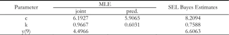
re-cord value were obtained under the SEL and LINEX loss functions under differ-ent values for v. Table 1A summarizes the results for ML and Bayes estimates when the SEL function is used. Table 1B, gives LINEX estimates for different values of v.
TABLE 1A
Bayes and Bayes SEL estimates
MLE Parameter
joint pred. SEL Bayes Estimates
c 6.1927 5.9065 8.2094
k 0.9667 0.6031 0.7588
y(9) 4.4966 6.6063
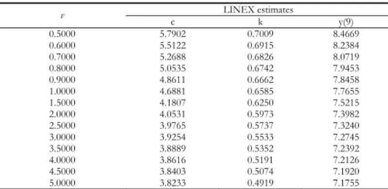
TABLE 1B
LINEX estimates
LINEX estimates v
c k y(9)
0.5000 5.7902 0.7009 8.4669
0.6000 5.5122 0.6915 8.2384
0.7000 5.2688 0.6826 8.0719
0.8000 5.0535 0.6742 7.9453
0.9000 4.8611 0.6662 7.8458
1.0000 4.6881 0.6585 7.7655
1.5000 4.1807 0.6250 7.5215
2.0000 4.0531 0.5973 7.3982
2.5000 3.9765 0.5737 7.3240
3.0000 3.9254 0.5533 7.2745
3.5000 3.8889 0.5352 7.2392
4.0000 3.8616 0.5191 7.2126
4.5000 3.8403 0.5074 7.1920
5.0000 3.8233 0.4919 7.1755
Figure 1 – Graph of prediction of c vs. .v
Figure 3 – Graph of prediction of y(9) vs. .v
Curve fitting reveals that there is an exponential relationship. Table 2, gives the exponential function and the R2 –adj.
TABLE 2
Relationship between the LINEX estimates and v
Parameter function R2 –adj
c c = 4.599exp(-1.836ν) + 4exp(-0.008864ν) 0.9987
k k = 0.158exp(-0.596ν) + 0.5933exp(-0.04103ν) 0.9999
y(9) y(9) = 2.878exp(-2.092ν) + 7.466exp(-0.00833ν) 0.9991
The values of R2 –adj are very close to 1, which implies almost a perfect
rela-tionship between each of the parameter estimates and v. Furthermore, one can predict the value of the LINEX estimator if he has decided on the value of v.
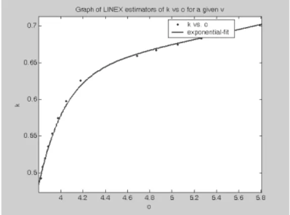
It is also of interest to plot the graphs of c vs. k, c vs. (9)y and k vs. (9)y when the values of v are specified. These graphs are shown below in Figures 4, 5 and 6.
Figure 5 – Graph of LINEX estimators of y(9) vs. c for a given v.
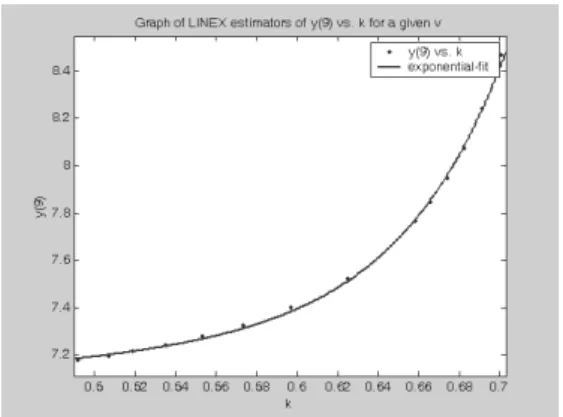
Figure 6 – Graph of LINEX estimators of (9)y vs. k for a given v.
Again, from curve fitting it is evident that there is an exponential relationship in each of these figures. Table 3, gives the functions and R2 –adj.
TABLE 3
Relationship among LINEX estimates
Parameter function R2 –adj
k k = 0.5292exp(0.04867c) – 2200000exp(-4.334c) 0.9977
y(9) y(9) = 4.847+0.6188 c 0.9930
y(9) y(9) = 6.904exp(0.07425k) + 0.00000exp(18.768) 0.9987
If one knows the estimate of one parameter, using the functions from Table 3 can estimate the remaining two.
Department of Mathematics MUSTAFA NADAR
Gebze Institute of Technology, Turkey
Department of Mathematics ALEXANDROS PAPADOPOULOS
REFERENCES
J. AHMADI, (2000), Record values, theory and applications. Ph.D. Thesis, Ferdowsi University of
Mashhad, Mashhad, Iran.
J. AHMADI, M. DOOSTPARAST, (2006), Bayesian estimation and prediction for some life distributions
based on record values, “Statistical Papers”, 47, vol. 3, pp. 373-392.
J. AHMADI, M. JOZANI, E. MARCHAND, A. PARSIAN, (2009), Prediction of k-records from a general class of
distributions under balanced type loss functions, “Metrika”, 70, vol. 1, pp. 19-33.
E.K. AL-HUSSAINI, Z.F. JAHEEN, (1992), Bayesian estimation of the parameters, reliability and failure
rate functions of the Burr Type XII failure model, “J. Statist. Comput. Simul.”, 41, pp. 1829-1842.
E.K. AL-HUSSAINI, Z.F. JAHEEN, (1995), Bayesian prediction bounds for the Burr Type XII failure
model, “Commun. Statist. Theor. Meth.”, 24, pp. 1829-1842.
E.K. AL-HUSSAINI, M.A. MOUSSA, Z.F. JAHEEN, (1992), Estimation under the Burr type XII failure
model based on censored data: A comparative study, “Test”, vol 1, pp. 33-42.
B.C. ARNOLD, N. BALAKRISHNAN, H.N. NAGARAJA, (1998), Records, John Wiley, New York. M.A.M ALI MOUSA, (2001), Inference and prediction for the Burr Type X model based on Records,
“Sta-tistics”, 35, pp. 415-425.
A.M. AWAD, M.Z. RAQAB, (2000), Prediction intervals for the future record values from exponential
distri-bution: comparative study, “J. Statist. Comput. Simul.”, 65, pp. 325-340.
P. BASAK, N. BALAKRISHNAN, (2003), Maximum likelihood prediction of future record statistic.
Mathe-matical and statistical methods in reliability, in B.H. Lindquist and K.A. Doksun (eds.), “Se-ries on Quality, Reliability and Engineering Statistics”, 7, Singapore: World Scientific Publishing, pp. 159-175.
I.W. BURR, (1942), Cumulative frequence functions, “Ann. Math. Statist.”, 13, pp. 215-232. K.N. CHANDLER, (1952), The distribution and frequency of record values, “J. R. Stat. Soc. Series B”,
14, pp. 220-228.
M. DOOSTPARAST, J. AHMADI, (2006), Statistical analysis for geometric distribution based on records,
“Computers & Mathematics with applications”, 52, pp. 905-916.
S.D. DUBBEY, (1972), Statistical contributions to reliability engineering, “ARL TR”, AD 774537,
pp. 72-0120.
S.D. DUBBEY, (1973), Statistical treatment of certain life testing and reliability problems, “ARL TR”,
AD 774537, pp. 73-0155.
W. FELLER, (1966), An Introduction to Probability Theory and its Applications, Vol. 2, second
edi-tion, John Wiley, New York.
S. GULATI, W.J. PADGETT, (1994), Smooth nonparametric estimation of the distribution and density
func-tions from record breaking-data, “Commun. Statist. Theor. Meth.”, 23, vol. 5, pp. 259-1274.
M.I. HENDI, S.E. ABU-YOUSSEF, A.A ALRADDADI, (2007), A Bayesian Analysis of Record Statistics from
the Rayleigh Model, “Intern. Mathem. Forum”, 2, vol. 13, pp. 619-631.
Z. F.JAHEEN, (2005), Estimation based on generalized order statistics from the Burr model.
Commun. Statist. Theor. Meth. 34:785-794.
D. MOORE, A.S. PAPADOPOULOS, (2000), The Burr Type XII distribution as a failure model under
various loss functions, “Microelectronics Reliability”, 40, pp. 2117-2122.
V. NEVZOROV, (2001), Records: mathematical theory, Translation of Mathematical Monographs.
“Amer. Math. Soc.”, 194, Providence, RI.
A.S. PAPADOPOULOS, (1978), The Burr distribution as a failure model from a Bayesian approach,
“IEEE Trans. Rel.”, R-27, vol. 5, pp. 369-371.
M.Z. RAQAB, J. AHMADI, M. DOOSTPARAST, (2007), Statistical inference based on record data from
H.R. VARIAN, (1975), A Bayesian approach to real estate assessment, in S.E. Finberg and A.
Zell-ner (eds.), “Studies in Bayesian Econometrics and Statistics” in Honor of J. L. Savege, North Holland, Amesterdam, pp. 195-208.
SUMMARY
Bayesian analysis for the Burr type XII distribution based on record values