Packet Classification for Core Routers: Is there an
alternative to CAMs?
Florin Baboescu, Sumeet Singh, George Varghese
Abstract— A classifier consists of a set of rules for classifying packets based on header fields. Because core routers can have fairly large (e.g., 2000 rule) database and must use limited SRAM to meet OC-768 speeds, the best existing classification algorithms (RFC, HiCuts, ABV) are precluded because of the large amount of memory they need. Thus the general belief is that hardware solutions like CAMs are needed, despite the amount of board area and power they consume. In this paper, we provide an alternative to CAMs via an Extended Grid-of-Tries with Path Compression (EGT-PC) algorithm whose worst-case speed scales well with database size while using a minimal amount of memory. Our evaluation is based on real databases used by Tier 1 ISPs, and synthetic databases. EGT-PC is based on a observation that we found holds for all the Tier 1 databases we studied: regardless of database size, anypacket matches only a small number of distinct source-destination prefix pairs. The code we wrote for EGT-PC, RFC, HiCuts, and ABV is publicly available [1], providing the first publicly available code to encourage experimentation with classification algorithms.
I. INTRODUCTION
The rapid growth of the Internet has brought great chal-lenges and complex issues in deploying high-speed networks. The number of users, the volume of traffic and the type of services to be provided are continually increasing. The increasing traffic demand requires three key factors to keep pace: high link speeds, high router data switching throughput and high packet forwarding rates. Although there are already solutions for the first two factors, packet forwarding continues to be be a difficult task at wire speeds.
Packet forwarding based on a longest matching prefix lookup of destination IP addresses is fairly well understood with both algorithmic and CAM-based solutions in the market. Using basic variants of tries and some pipelining, it is fairly easy to perform one packet lookup every memory access time, which can easily scale (beyond even today’s OC-768 speeds of 40 Gbps) to 100 Gps using 1 nsec SRAMs.
However, the Internet is becoming a more complex place to live in because of its use for mission critical functions executed by organizations. Organizations desire that their critical activities not be subverted either by high traffic sent by other organizations (i.e., they require QoS guarantees) or by malicious intruders (i.e., they require security guarantees). Both QoS and security guarantees require a finer discrimina-tion of packets based on fields other than the destinadiscrimina-tion that we call packet classification.
F. Baboescu, S. Singh and G. Varghese are with the Computer Science and Engineering Department, University of California, San Diego(UCSD), La Jolla, California. E-mail:{baboescu, susingh, varghese}@cs.ucsd.edu
Other fields a router may need to examine include source addresses (to forbid or provide different service to some source networks), port fields (to discriminate between traffic types such as Napster and say Email), and even TCP flags (to distinguish between say externally and internally initi-ated connections). Besides security and QoS, other functions that require classification include network address translation (NAT), metering, traffic shaping, policing, and monitoring.
The industry standard for classifier formats has come from Cisco ACLs, which consist of a number of rules. Each rule specifies a destination address prefix, a source address prefix, a protocol type or a wildcard, ranges for the destination and source port fields, and some values of TCP flags. The rules are arranged in order of priority and have an associated action (such as drop, forward, place in queueX etc.). Conceptually, a packet must be matched to the first (i.e., highest priority) rule that matches the packet.
Classifiers historically evolved from firewalls that were placed at the edges of networks to filter out unwanted packets. Such databases are generally small, containing 10-500 rules, and can be handled by ad hoc methods. However, with the DiffServ movement, there is potential anticipation [2] of classifiers that could support one hundred thousand rules for DiffServ and policing applications at edge routers. Thus while many classification algorithms [3], [4] work well for classifiers up to say 1000 rules, there is a real scaling problem for larger databases that is partially addressed by [5].
While large classifiers are anticipated for edge routers to enforce QoS via DiffServ, it is perhaps surprising that even within the core fairly large (e.g., 2000 rule) classifiers are commonly used for security. Emerging core routers operate at 40 Gbs speeds, thus requiring the use of limited SRAM to store state for any algorithmic solution. Unfortunately, the best existing classification schemes described in the literature (RFC [4], HiCuts [3], ABV [5]) require large amounts of memory for even medium size classifiers, precluding their use in core routers.
While these core router classifiers are nowhere near the anticipated size of edge router classifiers, there seems no reason why they should not continue to grow beyond the sizes reported in this paper. For example, many of the rules appear to be denying traffic from a specified subnetwork outside the ISP to a server (or subnetwork) within the ISP. Thus, new offending sources could be discovered and new servers could be added that need protection. In fact, we speculate that one reason why core router classifiers are not even bigger is because most core router implementations slow down (and do not guarantee true wire speed forwarding) as classifier sizes
increase.
Thus the general belief is that hardware solutions like Ternary CAMs are needed for core routers, despite the large amount of board space and power that CAMs consume [2], [6]. For a large number of designers, Ternary CAMs, which essentially compare a packet to every rule simultaneously, are the only solution.
There are several reasons to consider algorithmic alterna-tives to Ternary CAMs, however, some of which are stronger than others:
• Density Scaling: One bit in a TCAM requires 10-12 transistors while an SRAM requires 4-6 transistors. Thus TCAMs will also be less dense than SRAMs or take more area. Board area is a critical issue for many routers.
• Power Scaling:TCAMs take more power because of the parallel compare. CAM vendors are, however, chipping away at this issue by finding ways to turn off parts of the CAM to reduce power. Power is a key issue in large core routers.
• Time Scaling: The match logic in a CAM requires all
matching rules to arbitrate so that the highest match wins. Older generation CAMs took around 10 nsec for an operation but currently announced products appear to take 5 nsec, possibly by pipelining parts of the match delay.
• Extra Chips:Given that many routers like the Cisco GSR or the Juniper M160 already have a dedicated ASIC (or network processor) doing packet forwarding it is tempting to integrate the classification algorithm with the lookup without adding CAM interfaces and CAM chips. Note that CAMs typically require a bridge ASIC in addition to the basic CAM chip, and sometimes require multiple CAM chips.
• Rule Multiplication for Ranges: CAMs need to
repre-sent port ranges by several prefixes thus causing extra entries.
To see that this problem is not just of academic interest consider the following recent announcement by Cypress (a leading manufacturer of CAM chips) in EE Times [2]. Basi-cally, Cypress is considering shipping a chip that implements an algorithmic approach to classification to provide a lower cost, lower area, and lower power alternative to their CAMs. The article also mentions other companies such as Fast-Chip, EZchip, and Integrated Silicon Solution that are claiming algorithmic solutions.
II. PAPERCONTRIBUTIONS
Our paper has three main contributions: a new classifier characteristic, a new algorithm, and the first standardized comparison across a number of major algorithms.
• i, New Characteristic: Our paper studies the charac-teristics of core router classifiers used by Tier 1 ISPS. While previous studies have shown [4] that every packet matches at most a few rules, we refine this earlier observation to show that every packet matches at most a few distinct source-destination prefix pairs present in the rule set. In other words, if we project the rule set to
just the source and destination fields, no packet matches more than a small number of rules in the new set of projected rules. Note that this is emphatically not true for single fields because of wildcards: a single packet can match hundreds of rules when considering any one field in isolation.
• ii, New Algorithm:Based on the observation above, our paper introduces a new algorithm we callExtended Grid of Trie with Path Compression(EGT-PC)for multidimen-sional packet classification and evaluates it. While our EGT algorithm is inspired by the earlier grid-of-tries al-gorithm [7], it requires a significant extension. Briefly, the standard grid-of-tries assumes that any source-destination prefix pair(S1, D1)that is no more specific in both fields
than another pair(S2, D2)can be eliminated. While this
works for 2 field classification it does not work for more than 2 fields, and requires new machinery (e.g., jump pointers instead of switch pointers) for correctness. We had to experiment with a number of extension variants before finding one that did not result in storage replication and yet had good performance.
• iii, New standardized comparison: Previous work mostly compares the new algorithm presented in the paper with one other algorithm. Thus for example, the HiCuts paper [3] describes improvements over RFC [4]; similarly, the ABV paper [5] paper describes improve-ments over the Lucent bit vector scheme [8]. The code for each algorithm is also usually difficult to obtain. We have written code for each of these algorithms1and compared them using databases used by Tier 1 ISPs. We also do comparisons based on synthetic databases that preserve the structure of the smaller real databases that we have.2 Finally, our code is publically available on a web site described in the references. By making multiple classification algorithms publicly available we hope to encourage experi-mentation and improvements that can then be incorporated into revisions on the same web site.
III. PRIORWORK ANDSUMMARY OFRESULTS The packet classification problem is inherently hard( [8], [9], [3], [7], [4], [10]) from a theoretical standpoint. It has been shown [8] that in its fullest generality, packet classification requires either O(logk−1N) time and linear space, or logN
time andO(Nk)space, whereN is the number of rules, and kis the number of header fields used in rules.
Most practical solutions either use linear time [8] to search through all rules sequentially3, or use a linear amount of parallelism (e.g., Ternary-CAMs as in [11], [12]). Ternary CAMs are Content Addressable Memories that allow wildcard bits. Solutions based on caching [13] do not appear to work well in practice because of poor hit rates and small flow
1The RFC code is based on code graciously supplied to us by Pankaj Gupta 2Our databases are different from those in [5] because those databases were
largely edge databases as opposed to core databases. Our synthetic generation methodology is also very different from [5] in that we provide a simpler and more realistic model for generating large ISP classifiers.
3The scheme in [8] reduces classification to linear search on aN-bit vector
durations [14], and still need a fast classifier as a backup when the cache fails.
Several algorithms have been developed for the case of rules on two fields (e.g., source and destination IP address only). For this special case, the lower bounds do not apply (they apply only fork >2); thus hardly surprisingly, there are algorithms
that take logarithmic time and linear storage. These include the use of range trees and fractional cascading [8], grid-of-tries [7], area-based quad-trees [15], and FIS-trees [16]. While these algorithms are useful for special cases (such as measuring traffic between source and destination subnets), they do not solve the general problem of k−dimensional packet classification.
The papers by Gupta and McKeown [4], [3], [10] introduced a major new direction into packet classification research. Since the problem is unsolvable in the worst case, they look instead for heuristics to exploit the structure of the databases. They observed for the first time that a given packet matches only a few rules even in large classifiers. Baboescu and Varghese [5] also exploit this observation to reduce the search times for the algorithm described in [8]. Qiu et al [17] exploit the observation that any packet matches at most a few distinct values in each field to suggest backtracking trie search as a viable (though fairly slow) alternative.
Performance of Existing Schemes:In terms of the current state of the art (see comparisons later), it appears that RFC has the fastest search times (12 memory accesses using 16 bit chunks) but at the cost of a large amount of storage (for example, on a database of 2800 rules, RFC requires 24 Mbits of memory). HiCuts takes more memory accesses and requires less memory (e.g., 3 Mbits for the same database using 82 memory accesses).
HiCuts mostly works well. However, with the space factor of 4 used in the HiCuts paper, it is fast (82 memory accesses for a 2800 rules database) but requires a large amount of storage for databases (see DB3 below) in which there are
a large number of rules where the destination address is wildcarded, and a large number of rules where the source address is wildcarded. Using a lower space factor of 1, HiCuts tends to sometimes do better in storage but still does worse in time. In the case ofDB4,HiCuts−4uses more than3times
more memory than EGT −P C while the worst case search time is only slightly better:82vs.87while HiCuts−1uses about 16% less memory than EGT −P C but sacrifices the worst case search time which is now twice as large as the one for EGT −P C.
Besides these better results for existing core router databases,EGT−P C has three other characteristics that may make it more attractive than HiCuts.
• Predictability: It appears to be difficult to predict the performance of HiCuts on arbitrary database because there is no model to predict its performance. EGT − P C performance can be characterized in terms of the maximum number of rules that match a projection of the original rule set onto the source and destination fields.
• Scaling: EGT −P C appears to scale well to large databases.
• Patent issues: EGT − P C is not subject to patent
restriction unlike HiCuts which is patented. While this is not a fundamental issue, it does provide an important reason for looking for alternatives to HiCuts in practice. While RFC is very fast, its large amount of memory makes it hard to implement using limited SRAM. Thus for existing ISP databases none of the existing algorithms including HiCuts scale as well in both memory and time. Further, the EGT-PC scheme can easily be implemented using a small amount of SRAM.
More importantly, when we attempted to scale the database sizes to 100,000 while preserving their structure, EGT-PC took only slightly more memory accesses (at most 118) while preserving low storage4. Thus EGT-PC should scale well assuming that larger databases keep the same source-destination prefix characteristics of the Tier 1 ISP databases we studied.
Assuming a chip capable of around 32 memory accesses per minimum size packet (using say a 32 way pipeline), EGT-PC should allow the handling of large classifiers in 2-3 minimum size packet times in the worst-case. While this is not quite wire speed forwarding, such performance for large classifiers in some pathological cases seems adequate since most core routers today can also fall below wire speed forwarding for large classifiers.
A. Models and Metrics
Readers familiar with classification should skip the next section to get to the new material presented in the paper. In general, the job of a packet classifier is to categorize packets based on a set of rules. Rules are also sometimes called filters. The information relevant for classifying a packet is con-tained inK distinctheader fieldsin the packet. These header fields are denoted H[1], H[2], ..., H[K].
For example, the fields typically used to classify IPv4 packets are the destination IP address, source IP address, protocol field, destination port number, source port number, and protocol flags. The number of protocol flags is limited, so we can combine them into the protocol field itself.
Using these fields, a ruleF=(128.252.*, *, TCP, 23, *), for example, matches all traffic addressed to subnet128.252using TCP destination port 23, which is used for incoming Telnet; using a rule like this, a firewall may disallow Telnet into its network.
A classifier (also known as rule database or filter database) consists of N rules F1, F2, ..., FN. Each rule Fj is an array of Kvalues, where Fj[i]is a specification on thei-th header field. Thei-th header field is sometimes referred to as thei-th dimension. The valueFj[i]specifies what thei-th header field of a packet must contain in order for the packet to match rulej. These specifications often have (but need not be restricted to) the following forms: exact match, for example “source address must equal 128.252.169.16”; prefix match, like “destination address must match prefix 128.252.*”; or range match, e.g. “destination port must be in the range 0 to 1023.”
4However, a linear increase in the memory space that it is used may be
obtained if the number of distinct prefixes in the database scale as well with the the number of rules in the database.
Each rule Fj has an associated directive dispi, which specifies the action to perform for a packet that matches this rule. This directive may indicate whether to block the packet, send it out a particular interface, or perform some other action. A packetPis said tomatcha ruleF if each field of P matches the corresponding field ofF. For instance, let
F = (128.252.∗,∗, T CP,23,∗) be a rule withdisp=block. Then, a packet with header (128.252.169.16, 128.111.41.101, TCP, 23, 1025) matches F, and is therefore blocked. The packet (128.252.169.16, 128.111.41.101, TCP, 79, 1025), on the other hand, doesn’t match F.
Since a packet may match multiple rules in the database, we associate a cost for each rule to resolve ambiguous matches. The packet classification problem is to find the lowest cost rule matching a given packet P.
B. Performance metrics for packet classification
The two main metrics for packet classification are speed in memory accesses and memory. A secondary metric could be the number of fields that can be handled; some applications require more than 5 fields although we will only consider 5 field classifiers in this paper.
Speed:The goal of packet classification is to ideally classify packets at wire speed, which means that for each packet a decision is to be made in the time we have for handling a minimum size packet. At OC-192 rates of 10 Gbps and using 40 byte packets, a decision must be made in 32 nsec.
In practice, this is tricky for several reasons. First, even the definition of minimum packet size is debatable: there are a few rare packets that arrive in with sizes of 30 bytes or less; while most studies use 40 byte minimum size packets (since packets with TCP, IP, and Data link headers are at least this size) some vendors aim for a 64 byte packet sizes with a small queue to handle bursts of smaller sizes. Second, some packet processing events like handling encapsulated packets or multiple levels of label stacking may require multiple lookups that cannot strictly be handled at line speed for a minimum packet size. Thus some relaxation of strict wire speed processing limits for say packet processing may be acceptable (especially when using a large classifier); indeed, this appears to be true for most core routers today.
Speed is measured in terms of memory accesses. Often a wider memory access can reduce the number of memory accesses required. We will assume a 32 bit wide memory. Many of the algorithms described here (especially the two leading contenders HiCuts and EGT) can benefit from wider words, but we normalize our results to 32 bit words.
Memory size: On-chip SRAM for semi-custom ASICS is at most 32 Mbits today. Since on-chip SRAM provides the fastest memory (around 1 nsec), one would ideally like the memory of a classification algorithm to scale with the size of an on-chip SRAM. For example, the RFC sizes of 24 Mbits for a 2800 size table (see results later) tend to rule out RFC for high speed implementations.
Update complexity is generally not an issue for core routers as rules are rarely changed. On the other hand, edge routers that do stateful filtering or intrusion detection systems that
dynamically identify certain flows to be tracked may indeed require faster updates. We do not consider update complexity in this paper.
IV. BRIEFREVIEW OFRFCANDHICUTS
In this section we briefly describe two of the previous algorithms that we compare against our new EGT scheme. We describe HiCuts in some detail as it is the strongest contender for the core router databases we examined. We describe our new algorithm in the next Section. In order to provide examples, let’s consider the small firewall database in the Figure 1. The example contains twelve rules on five fields. A. Recursive Flow Classification(RFC)
The first algorithm we consider is RFC [4]. Gupta and McKeown [4] have invented a scheme called Recursive Flow Classification (RFC). RFC is really an improved form of cross-producting that significantly compresses the cross-product table at a slight extra expense in search time. The scheme works by building larger products from smaller cross-products; the main idea is to place the smaller cross-products into equivalence classes before combining them to form larger cross-products. This equivalencing of partial cross-products considerably reduces memory requirements, because several original cross-product terms map into the same equivalence class.
In Figure 2 we apply the equivalence cross-producting to the first two columns in the example in Figure 1. A two dimensional table is built based on the unique prefixes in each of the first two fields. In this case the result is7distinct values which is close to the number of unique prefixes in the second field.
Prefix matching on a large field can be performed by splitting it up and treating it as several smaller fields. This is useful for fields exceeding 16 bits in length, since a field
W bits in size requires a table of size 2W to map values to equivalence classes. We use the field value of 16 bits suggested in the RFC paper.
B. Hierarchical Intelligent Cuts (HiCuts)
HiCuts was introduced by Gupta and McKeown in [3]. The scheme is based on a precomputed decision tree which is traversed for each packet that need to be classified in order to identify the matching rule which is always located in a leaf node. Each leaf node stores a small number of rules which are linearly searched in the last step. It is a remarkably effective algorithm and so is worth describing in more detail.
In HiCuts each node can be regarded as a k−dimensional region cut up into a set ofncsmaller regions using heuristics which try to take into account the structure of the classifiers. The size of a region is given by the range covered by the region. For example the root node for a 5−tuple (IP Source and Destination, Port Source and Destination, Protocol) may be seen as the region [0,232 −1]X[0,232 −1]X[0,216 −
1]X[0,216−1]X[0,28−1]. The set of rules which intersect
Rule F ield1 F ield2 F ield3 F ield4 F ield5 ACT ION
F0 000∗ 111∗ 10 ∗ U DP act0
F1 000∗ 111∗ 01 10 U DP act0
F2 000∗ 10∗ ∗ 10 T CP act1
F3 000∗ 10∗ ∗ 01 T CP act2
F4 000∗ 10∗ 10 11 T CP act1
F5 0∗ 111∗ 10 01 U DP act0
F6 0∗ 111∗ 10 10 U DP act0
F7 0∗ 1∗ ∗ ∗ T CP act2
F8 ∗ 01∗ ∗ ∗ T CP act2
F9 ∗ 0∗ ∗ 01 U DP act0
F10 ∗ ∗ ∗ ∗ U DP act3
F11 ∗ ∗ ∗ ∗ T CP act4
Fig. 1. A simple example with12rules on five fields.
F ield1/F ield2 000∗ 0∗ ∗
111∗ 110001110011 =C0 000001110011 =C1 000000000011 =C2
10∗ 001110010011 =C3 000000010011 =C4 C2
1∗ C4 C4 C2
01∗ 000000001111 =C5 C5 C5
0∗ 000000000111 =C6 C6 C6
∗ C2 C2 C2
Fig. 2. Forming the partial cross-products of the first two fields in Figure 1 and assigning them into the same equivalence class if they have the same set of matching rules.
A similar ideea with bit tests replacing range tests, was described by T. Woo in [10]. Much more [10] introduces one more degree of freedom in building the decision tree: it allows to arbitrarily interleave the bit tests from all fields. Thus the root of the trie could test for (say) Bit 10 of the source field; if the bit is 0, this could lead to a node that tests for say Bit 22 of the port number field. The schemes in [10] and [3] build the final decision tree usinglocal optimizationdecisions at each node to choose the next bit to test.
In what follows, we describe HiCuts in more detail using an example.
Picking the number of regionsnca node is split into may be done based on several heuristics which try to make a tradeoff between the depth of the decision tree and implicitly the search time versus the memory space occupied by the decision structure. The dimension on which a cut may be executed may be chosen either to:(1) minimize the maximum number of rules into any partition, or (2) maximize the different number of specifications in one dimension, etc. Picking the right number of partitions(nc)to be made affects the overall memory space. The algorithm tunesncas a function of a space measure. In order to do this it uses to parameters: (1) binth and (2) spfac.
Figure 3 shows a decision tree for the Example in Figure 1. Let’s assume that a packet with the header (0010,1101,00,01, T CP) needs to be classified. The path followed by this packet is shown in red in Figure 3. In the first node, markedA, based on the value in its first field, the packet is directed to the node marked B. Node B uses information in the second field to direct to a leaf node containing a small
list of rules which may be a possible match. In this caseF7
is the lowest cost rule matching the packet.
F9 F10 F11
F8 F9 F10
F7 F10 F11
F7 F10 F11
F7 F10 F11 (0010, 1101, 00, 01, TCP)
A
B Field 2, 4
F11
Field 4, 4 Field 3, 4
Field5, 2 F3
F7 F10 F11
F2 F7 F10 F11
F4 F7 F10 F11
F1 F7 F10 F11
F7 F11
F0 F5 F6 F10
Fig. 3. A decision tree is built for the database of Figure 1. The dimension on which a cut is made is associated with the field which has the largest number of unique values. For example the first node is cut along the first field.
V. CHARACTERISTICS OF REAL LIFE CLASSIFIERS Each designer of packet classification heuristics faces the same problem; he or she must know the characteristics of large rule databases. In this section we analyze 4 real life classifiers which are used by several large Tier 1 ISPs. While real databases were also used in [5] and [3], [4], the databases in [5] are small and only reflect firewall applications which are not a good characterization of core router databases. Similarly, it is unclear whether the databases in [3], [4] were mostly from edge routers.
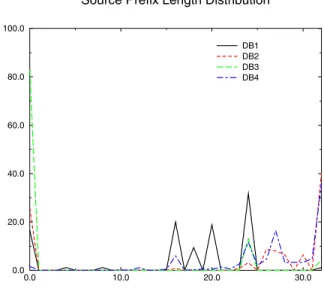
The number of rules in the classifiers varies from85to2800 as is shown in Figure 9. All the classifiers are five dimensional
with the IP source and destination field represented as prefixes while the port fields are represented as ranges. The prefix length distribution for both IP source and destination fields is given in Figures 4 and 5.
With the exception of one database which appears to have rules connecting subnetworks (prefix lengths with values of 16−24) all the other databases have the similar maximums at length of 0, 16, 24 and 32. The distribution is very different from the prefix distribution in publicly available routing tables( [18]) which is described in [5].
The performance of many classifier algorithms are strictly dependent on the largest number of valid prefixes that may be seen on a path from the root to a leaf in a trie that is generated using all the prefixes. The values for this number are between 3 and7 for source and destination address tries. However if we consider the source tries associated with any particular destination trie, then the number is even smaller: between2 and4.
The number of rules matching all five fields is somewhere between3and5. This result is consistent with the result given by Gupta and McKeown in [4], [3]. A value of 3 is easily achieved by a classifier which contains a default rule to be executed on all packets, a second rule to be executed on all the packets carrying a TCP message, and a third rule to be executed on all packets for an establishedTCP connection.
Analyzing the number of IP source and destination pairs only in the rule set we notice that the most common ones in order of their occurrence are:
• i.32−bit IP source to32−bit IP destination. This form of rule appears to be protecting particular ISP servers/routers from particular hosts. Of course, these rules are qualified by port fields that specify the traffic type.
• ii.Anything (wildcarded) to 32−bit IP destination. This form of rule appears to be protecting servers from being reached from the external world.
• iii.16 or 24 bit network source address to 32−bit IP
destination. This form of rule is similar to the first type of pattern except generalized to protecting servers from particular subnets.
• iv.24−bit network source address to anything. This form of rule simply forbids certain subnetworks for certain specified traffic types.
To test scaling later, we use a much simpler synthetic database generation algorithm than [5]. Since each database we studied is quite different in patterns and distribution of length tuples, we used each database as a model to synthesize larger databases by simply replacing each IP address or prefix in a rule by other addresses while keeping other fields the same. This seems to be a reasonable model of an ISP growing in servers to be protected and subnetworks to be protected against.
A. IP Source-Destination matching characteristic
The key observation that forms the basis of our new algorithm is as follows.
Source-Destination Matching: For all our databases, we computed the BV bitmap on all possible source and destination
0.0 10.0 20.0 30.0
0.0 20.0 40.0 60.0 80.0 100.0
Source Prefix Length Distribution
DB1 DB2 DB3 DB4
Fig. 4. Prefix Distribution in the IP source field.Prefix length is repre-sented on the horizontal axis while the percentage of entries with a given prefix length is given on the vertical axis. The graphs have a maximum on the lengths of0,16,24and32.
0.0 10.0 20.0 30.0
0.0 20.0 40.0 60.0 80.0 100.0
Destination Prefix Length Distribution
DB1 DB2 DB3 DB4
Fig. 5. Prefix Distribution in the IP destination field.Prefix length is represented on the horizontal axis while the percentage of entries with a given prefix length is given on the vertical axis. The graphs have a maximum on the lengths of0,16,24and32
prefix values. Then for each possible source-destination prefix pair (crossproduct) we computed the intersection of these bitmaps and counted the number of rules that matched a given packet when considering only the first two fields. We found that for 99.9% of the source-destination crossproducts, the number of matching rules was5or less. Even in a worst case sense, no crossproduct (and hence packet) for any database matches more than 20 rules when considering only source destination field matches.
Notice that this observation implies that the number of distinct source-destination prefix pairs matching a packet is even less than 20 because there can be several rules that share
the same source-destination prefix pair. This observation is true for the smallest to the largest database of around 2800 rules. We expect it to remain approximately true even as databases scale because the number of overlapping prefixes (e.g., of lengths 0, 24, 32) are so limited in each of the source and destination fields.
Note that the small number of matches is not true when one considers only the source or destination fields because of the large numbers of wildcards in each field.
VI. EXTENDING2DSCHEMES
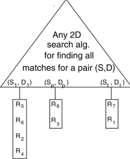
A number of algorithms simply use linear search to search through all possible rules. This scales well in storage but poorly in time. The source-destination matching observation leads to a very simple idea shown in Figure 6 to use source-destination address matching to reduce the linear searching to all rules corresponding to source-destination prefix pairs in the database that match the given packet header. Since mostly 5 and at most 20 rules will match any packet when considering only the source and destination fields, this will reduce the number of rules to be searched to be between 5 and 20. Thus we have linear searching among a pruned space of around 20 rules compared to linear searching the entire database (e.g., 2800 rules in our large databases).
R R R 5
6
2
4
R7 1 R8
R3 Any 2D search alg. for finding all matches for a pair (S,D)
R
R
1 1 p p t t
(S , D ) (S , D ) (S , D )
Fig. 6. Extending two dimensional schemes
The main idea is depicted in Figure 6. The idea is to use any efficient two dimensional matching scheme to findallthe distinct source-destination prefix pairs (S1, D1). . .(St, Dt) that match a header. For each distinct pair(Si, Di)there is a linear array or list with all rules that contain (Si, Di)in the source and destination fields. Thus in the figure, we have to traverse the list at(S1, D1)searching through all the rules (in
reality only the other fields such as port numbers) forR5,R6,
R2 andR4. Then we move on consider the lists at(S2, D2),
etc.
Notice that this structure has two important advantages:
• Each rule is only represented once without replica-tion.However, one may wish to replicate rules to reduce the number of source-destination pairs considered to reduce search times.
• The port range specifications stay as ranges in the
in-dividual lists without the blowup associated with range translation in say CAMs, BV, and ABV.
Since the Grid-of-Tries implementation by Srinivasan et al [7] is one of the most efficient two dimensional schemes described, we now instantiate this general schema by using grid-of-tries as the 2D algorithm in Figure 6
A. Extended Grid-of-Tries(EGT)
In a naive generalization of a k-dimensional trie we either pay a large price in memory or we may be forced to do backtracking and we pay a large price in time [17]. However, we may eliminate part of the waste of backtracking by using precomputation. This basic technique was introduced in the two dimensional trie implementation using grid of tries [7].
However one can immediately see that the approach in grid of tries cannot be generalized ink, k >2dimensions. This is because the grid of tries algorithm assumes that a rule may have at most two fields. If two rules are a match for a packet, then the most specific rule is picked. This observation allows the replacement of the backtracking mechanism with switch pointers. By using aswitch pointer in any failure point in the source trie, it allows the search to jump to the next possible second dimension trie which may contain a matching rule.
Our goal is that for each packet headerH = (H1, H2, . . .)
to be able to identify the set of rules F such that F = {F[i]|F1[i]≤H1∩F2[i]≤H2}.
In our extended grid of trie structure, a first trie is associated with the first dimension in the rule database. For every valid prefix node in this trie a special node is created. Each of these nodes contains a link to a trie which contains values from the second dimension field. For example, if the node in the first dimension trie is associated with a prefixP1 then the second dimension trie nodes is generated using all the second dimension field prefixes P2[i] from the rules Fi = (P1[i], P2[i], . . .), i= 1. . . N in the database.
A nodeX in the second dimension trie which is associated with a valid prefix P2 is appended with a list of rules which correspond to rules that match P1 and P2 in the first two dimensions. A node also contains a list of pointers to all the valid prefixes nodes which are a prefix of P2. Thus node X
knows the list of all the rules F[i] = (P1[i], P2[i], . . .) for whichP1[i] =P1 andP2[i]P25. However, a rule occurs in exactly one position.
A different approach is to keep in each node associated with a valid prefixP2the list of rulesF[i]which haveP1in the first field and in the second field a prefix P2[i] which is either an exact match or a prefix ofP2. We discuss these two approaches when we analyze the scheme behavior on real classifiers.
At this point, for each packet with a header H =
(H1, H2, . . .) we can identify the set of rules F =
{F[i]|F[i] =(P1, P2[i], . . .)}whereP1is the longest matching prefix ofH1for which at least a ruleFi= (P1, . . .)exists and P2[i] if exists isP2[i] H2. In order to get all the rules F
such thatF ={F[i]|F1[i]H1∩F2[i]H2} is necessary to
5P
traverse all the tries associated with prefixes in the first field that are prefixes of the fieldH1of the packet header. However
this requires backtracking in which case we pay a large price in time.
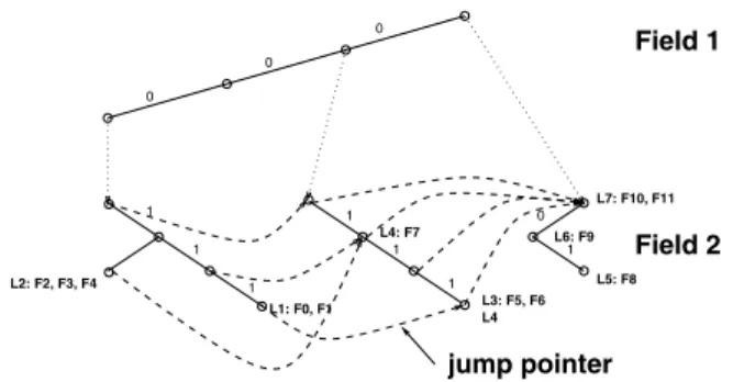
In order to avoid the backtracking we follow an approach inspired by but different from [7]: we introduce at each failure point in the second dimension trie a jump pointerto directly allow the search to jump to the next possible second dimension trie that may contain a matching rule. If the node in which we inserted a jump pointer is associated with a prefix P2 in the
second dimension trie, the jump is either to a node associated with a valid prefix P that is either shorter or equal withP, if such a node exist, or to a regular node which is the longest matching prefix of P2, otherwise.
Figure 7 shows the extended grid of tries for the database in Figure 1. Let’s consider the search for rules that match a packet header(0000,1100, . . .). The search in the first dimension trie
gives P1= 000 as the best match. So we start the search for
finding the matching prefix associated with the second value in the header 1111. We do not find a match in this trie. The search fails in the node 11. However a jump pointer allows the search to continue further into the trie associated with the prefix0∗in the first dimension. The search in this trie provides 1∗ as the longest matching prefix and one ruleF7 as being a matching rule. Once the search fails again in this dimension a jump pointer brings us to the last node corresponding to ∗,∗. This last node adds two more rules to the list making the final matching list to be: F7, F10, F11.
The worst search time for the scheme can be proved to be:
W + (H + 1)∗W = (H + 2)∗W where W is the time to find the best prefix in a trie andH is the maximum length of the trie, H = 32 for IP addresses. However, we expect that the worst case scenario does not occur in practice. Instead we expect the worst case search time to be on the order L∗W
withL being a small value.
We can also reduce W by using compressed multibit tries [19] instead of using 1-bit tries. If we use k−bit expan-sion, the depth of the trie reduces to W/kand so the lookup time goes down correspondingly without a corresponding 2k increase in storage that would be incurred by uncompressed tries.
The bottom line is that using multibit tries, the time to search for the best matching rule in an arbitrarily large multidimensional database could effectively reduce toktimes the time to do IP lookups using multibit tries, withkassumed to be a small constant, plus the time to search through a small list of rules.
B. Extended Grid of Trie with Path Compression
We further improve the Extended Grid of Trie algorithm by using Path Compression [20]. This is a standard compression scheme for tries in which single branching paths are removed. Figure 8 shows how the path compression is applied to the tries in the Figure 7.By doing so a trie with N leaf nodes can be compressed into a trie with at most 2N −1 nodes. Further improvement may be gained by applying both path compression as well as the compression techniques introduced in [19].
0
0
0
1
1
1 1
1
1 0
1
L2: F2, F3, F4
L1: F0, F1 L4: F7
L3: F5, F6 L4
L6: F9
L5: F8 L7: F10, F11
Field 1
Field 2
jump pointer
Fig. 7. Improving the search cost with the use ofjump pointersin the extended grid of tries. The tries are generated using the database in Figure 1.
0
1 11 0
1 11
0 1 L2: F2, F3, F4 L1: F0, F1
L4: F7
L3: F5, F6 L4
L5: F8 L6 L6: F9
L7: F10, F11 00
path compressed
Field 1
Field 2
Fig. 8. Reducing the time of the trie traversal by applying path compression to the tries in Figure 7.The tries are generated using the database in Figure 1.
VII. METHODOLOGY
In this section we describe how the EGT algorithm can be implemented, and how it performs on both real life databases and synthetically created databases. Note that we need synthet-ically created databases to test the scalability of our scheme.
First, we consider the complexity of the preprocessing stage and the storage requirements of the algorithm. Then, we consider search performance and we relate it to the perfor-mance of other algorithms: RFC, HiCuts, BV and ABV. The speed measure we use is the worst case number of memory accesses to be executed across all possible packet headers. Fortunately, computing this number does not entail generating all possible packet headers. This is because packet headers fall into equivalence classes based on distinct cross-products [7]; a distinct cross-product is a unique combination of distinct prefix values for each header field.
Since each packet that has the same cross-product is matched to the same nodeNi(in trieTi) for each fieldi, each packet that has the same cross-product will behave identically. Thus it suffices to compute worst case search times for all possible cross-products.
One can easily see that our algorithm has a worst case behavior when it may need to traverse a very large number of tries that are associated with the second dimension field. However pathological cases for which the heuristics experi-ence the worst behavior may be found for all the algorithms we presented. Therefore in this paper we focus on the worst case search time for a series of realistic test databases.
A. Experimental Platform
We used two different types of databases. First we used a set of four core router databases that we obtained from several large Tier 1 ISPs. For privacy reasons we are not allowed to disclose the name of the ISP or the actual databases. Each entry in the database contains a 6 −tuple (source IP prefix, destination IP prefix, source port number(range), destination port number(range), protocol and action). We call these databasesDB1. . . DB4. The database characteristics are
discussed in Section V.
The second type of databases is generated using the real life databases as a starting point. We extend each of the original databases by randomly generating prefixes for the first two fields with the same length distribution as in the original one. We also maintain the distribution for the last three fields.
B. Performance Evaluation on Real Life Core Router Databases
We experimentally evaluate all the algorithms on a number of four real life core router databases DB1, . . . , DB4. The rules in the databases are converted into prefix format using the technique described in [7] for the evaluation of the BV and ABV algorithms. The memory space that is used by each of them can be estimated based on the number of nodes in the tries, and the number of nodes associated with valid prefixes in the case of BV and ABV.
In the case of EGT we also need to take into account the sizes for the list as well as the jump pointers. We use words of size32bits and aggregate size of32forABV. In the case of
RF C at each level if the number of unique elements isN we uselog2Nbits for an index into that level. Therefore for each
table X∗Y the total memory size in bits isX∗Y ∗log2N.
Our results are summarized in Figure 9.
Both the search time and memory space inHiCuts[3] are dependent on two parameters which may be tuned: (1)space factor (spfac)- which determines the amount of total memory space that will be allocated on the decision tree and a (2) threshold(binth)(a node with fewer than binth rules is not partitioned further). [3] makes the observation that the tree depth is inversely proportional to binth and spfac while the total memory space is proportional with spfac and inverse proportional to binth. The results in Figure 11 and Figure 9 are for HiCuts−4:(binth= 10,spf ac= 4)andHiCuts−
1:(binth= 10,spf ac= 1).
In the case of three databases the memory space occupied byHiCuts−4(the value used in the original HiCuts paper) is an order of magnitude larger than the memory space occupied by the EGT −P C. However, by tuning the space factor parameter(spfac) to a value of1 corresponding to optimizing
HiCuts for memory space, the overall space occupied by
HiCuts is comparable in size withEGT for three databases while in the case ofDB3it is still about 7times higher than
EGT−P C.DB3 shows a database type which may hurt the performance of theHiCutsheuristics. In this case the height of the decision tree that is generated by HiCuts stays the same when spf acis changed from1 to4. This is because of
a set of rules which gets replicated in a majority of the leaf nodes.
In the case of both BV andABV notice the increase in the (aggregated) bit vector size with the number of rules in the database contributes to a higher increase in the overall memory size, being multiplied with the total number of valid prefix nodes in all the tries. However, not keeping the bits in the original bit vector which are associated with an aggregate bit with the value0 may reduce the memory usage ofABV. While this optimization can reduce the memory size ofABV, we have not shown its effect here. The results for RF C
confirm the assumption in [4] that despite of a worst case scenario in which an implementation may take O(Nk−1)
memory space, in reality the memory space occupied by the algorithm’s search structure is smaller.
Overall, as expected, RF C occupies by far the largest memory space. On the other side in terms of lowest memory space EGT −P C and HiCuts are the main competitors.
EGT −P C in general is the one with the best use of space. However, when HiCuts is optimized for memory space it comes close toEGT −P C but is slower with an worst case search time that is2−3times slower than EGT−P C.
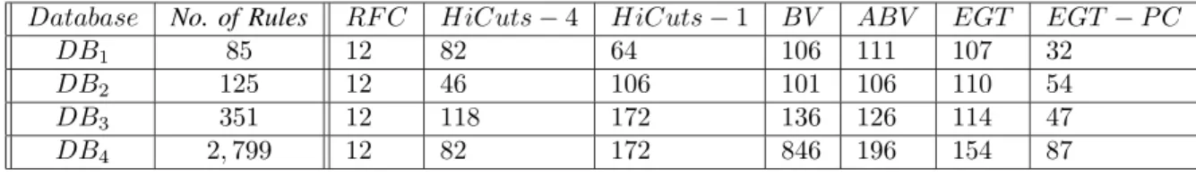
We also evaluate the performance of the five algorithms in terms of worst case lookup time on the core router databases. The results are shown in Figure 11.
As anticipatedRF Chas the best search time with a number of 12 memory accesses. The results in Figure 11 shows that classifying packets withABV has benefits when the number of memory entries in the database is large. In this case the search time for ABV is more than four times faster than in
BV even without rule rearrangement. However, if the number of rules is small, on the order of hundreds, the phenomenon of false matching described in [5] may limit the performance of ABV.
The search time in EGT −P C is mostly due to the several traversals of the tries. The worst case search time using
EGT −P C is on the same order of magnitude as HiCuts
when HiCuts is optimized for speed. However the memory space occupied byEGT −P C is on an order of magnitude smaller than any other analyzed heuristic with the exception of HiCuts optimized for a space factor of1. In this caseHiCuts
andEGT −P C occupy similar memory space sizes. C. Performance evaluation on synthetic generated databases
In this section we want to investigate the scalability of
EGT−P C. In order to do so we generated databases with a large number of rules between5,000 and100,000. The first
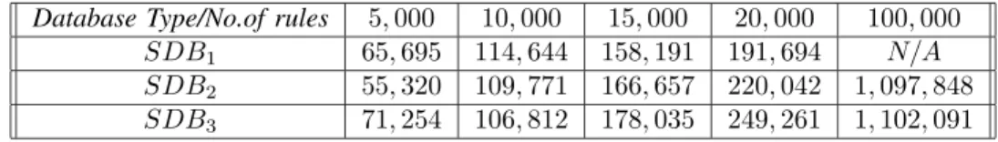
two types of databases,SDB1andSDB2are generated using as a generator the two longest real core router databases. The last type of database,SDB3are generated using a combination of all four real core router databases as a generator. Figure 13 shows the size of the memory occupied byEGT−P C while the number of rules in the classifier increases from 5,000 to 100,000.
The results prove that the memory space occupied by EGT − P C scales linearly in number of rules. Of course, this should be taken with a grain of salt because the
Database No. of Rules RF C HiCuts−4 HiCuts−1 BV ABV EGT EGT −P C
DB1 85 55,202 11,608 1,346 1,496 1,572 3,174 1,168
DB2 125 114,080 10,704 1,986 1,530 1,606 3.935 1,472
DB3 351 100,991 64,541 19,001 4,452 4,651 3,845 2,261
DB4 2799 747,271 117,801 25,543 276,604 285,099 75,376 30,753
Fig. 9. The total memory space occupied by the search structure in all 6 heuristics RFC, HiCuts(spf ac= 1,4), BV, ABV, EGT and EGT-PC for the four core router databases. The size is in memory words, one memory word is32bits.
Database EGT EGT−P C
Trie List Total Mem. Trie List Total Mem.
DB1 3,019 155 3,174 1,013 155 1,168
DB2 3,713 222 3,935 1,250 222 1,472
DB3 3,339 506 3,845 1,755 506 2,261
DB4 70,710 4,666 75,376 26,087 4,666 30,753
Fig. 10. The total memory occupied by both EGT and EGT-PC used with real life databases. The size is in memory words. One memory word is 32bits.
Database No. of Rules RF C HiCuts−4 HiCuts−1 BV ABV EGT EGT−P C
DB1 85 12 82 64 106 111 107 32
DB2 125 12 46 106 101 106 110 54
DB3 351 12 118 172 136 126 114 47
DB4 2,799 12 82 172 846 196 154 87
Fig. 11. The total number of memory accesses for a worst case search in all 5 heuristics RFC, HiCuts(spf ac= 1,4), BV, ABV, EGT and EGT-PC for the four core router databases. One memory access is one word. One word is32bits.
large database generation methodology preserves the source-destination structure of the original databases. If this assump-tion does not hold as databases scale up,EGT−P C will not scale. However, we have not seen any experimental evidence that this is not the case.
The worst case scenario for a search using EGT −P C is shown in Figure 12. In the case ofSDB3 with100,000rules
it takes about118memory accesses. This corresponds to about 5 trie traversals plus the selection of roughly30rules that are a match. In the case of SDB2 with 100,000 in the worst case it takes98memory accesses due to four one dimensional lookups and the selection of about 17rules.
VIII. CONCLUSION
Packet filter classification has received tremendous atten-tion( [8], [5], [7], [4], [3], [17], [15], [16], [10]). Unfortunately, despite the vast amount of previous work, there does not appear to be a good algorithmic solution when rules contain more than 2 fields. At the same time, classification is an extremely important problem with several vendors, including Juniper, allowing the use of filter-based actions for purposes such as accounting and security. While Ternary CAMs [11] offer a good solution in hardware for small classifiers, they may use too much power and board area for large classifiers. Thus it is worth looking for alternatives [2] to CAMs.
Because real-life classifiers have considerable structure, [4] observed that such structure could be exploited to yield heuristics that beat the worst-case bounds on real databases. The primary observation till this paper was [4] that each packet only matches a few rules. Our paper starts with a fresh
observation driven by data we observed: each packet does indeed match only a few rules, but it also matches only a few rules when the rules are projected to only the source and destination fields. Thus even for large classifiers, if one can find all the source-destination prefix pairs that match a packet, one need only linearly search through a set of 20 possible rules.
This suggests that any efficient two-field classification scheme can be extended with a small amount of linear search to general classifiers. The only catch is that the two-field scheme has to find matches, and not eliminate less specific matches. Thus, while this suggested starting with the grid-of-tries, we had to modify it using jump pointers to compute all matches, losing worst case guarantees on even the search time for 2-field search.
Despite this,EGT −P C works very well compared to all other algorithms. Its worst case search times are on the same order as for the HiCuts optimized for speed while its memory storage requirements are on the same order as for HiCuts optimized for space. Therefore we consider thatEGT −P C
provides a reasonably fast algorithm with minimal storage requirements that can fit into on-chip SRAM. Much more,
EGT −P C has the advantage of being more predictable, of not having any patent restrictions, and potentially allowing simple further improvements using compressed multibit tries as in [19]. We are working on the use of multibit tries, compressed versions of the lists, and the use of wide words to further reduce the space and time of EGT-PC. Our paper leaves open the issue of modifying other 2 field algorithms such as [16], [15], [8], [5] to achieve better performance. The lack of
Database Type/No. of rules 5,000 10,000 15,000 20,000 100,000
SDB1 62 96 114 155 N/A
SDB2 87 92 93 93 98
SDB3 106 101 100 109 118
Fig. 12. The total number of memory accesses for a worst case search for EGT-PC for synthetic databases. The number of entries is changed between5000and100,000. One memory access is one word and one word is32bits.
Database Type/No.of rules 5,000 10,000 15,000 20,000 100,000 SDB1 65,695 114,644 158,191 191,694 N/A
SDB2 55,320 109,771 166,657 220,042 1,097,848
SDB3 71,254 106,812 178,035 249,261 1,102,091
Fig. 13. The total memory occupied by EGT-PC used with synthetic databases. The number of entries is changed between5000and100,000. One memory word is32bits.
standardized comparisons has led us to place all the code we implemented on a public repository [1]. As others tinker with these algorithms, we believe that even better algorithms will be found and the state of the art will improve further. The use of packet classification is not confined to routers: from personal firewalls to web load balancing using URLs, better and open source code for classification can help improve a number of applications in software and hardware.
ACKNOWLEDGMENT
This work was supported through a NSF grant ANI 0074004 and a grant from NIST for the Sensilla project.
REFERENCES
[1] S. Singh and F. Baboescu, “Packet classification repository.” [Online]. Available: http://ial.ucsd.edu/ classification
[2] C. Matsumoto, “Cam vendors consider algorithmic alternatives,” in EETimes, may 2002.
[3] P. Gupta and N. McKeown, “Packet classification using hierarchical intelligent cuttings,” inProc of Hot Interconnects VII, august 1999. [4] ——, “Packet classification on multiple fields,” inProc of ACM
Sig-comm’99, september 1999.
[5] F. Baboescu and G. Varghese, “Scalable packet classification,” inProc of ACM Sigcomm’01, september 2001.
[6] P. Gupta and N. McKeown, “Algorithms for packet classification,” in IEEE Network Special Issue, vol. 15, no. 2, march 2001.
[7] V. Srinivasan and al, “Fast and scalable layer 4 switching,” inProc of ACM Sigcomm’98, september 1998.
[8] T. V. Lakshman and D. Stidialis, “High speed policy-based packet forwarding using efficient multi-dimensional range matching,” inProc. of ACM Sigcomm ’98, sept 1998.
[9] V.Srinivasan, S.Suri, and G.Varghese, “Packet classification using tuple space search,” inProc of ACM Sigcomm’99, september 1999. [10] T. Woo, “A modular approach to packet classification: Algorithms and
results,” inINFOCOM, 2000.
[11] Memory-memory, 2000. [Online]. Available: http://www.memorymemory.com
[12] S. Iyer and al, “Classipi:an architecture for fast and flexible packet classification,” inIEEE Network Spec. Issue, vol. 15, no. 2, 2001. [13] J. Xu and al., “A novel cache architecture to support layer-four packet
classification at memory access speeds,” inProc. of Infocom, mar. 1999. [14] C. Partridge, “Locality and route caches,” in Proceedings of NSF
Workshop, ISMA, feb 1999.
[15] M. M. Buddhikot and al, “Space decomposition techniques for fast layer-4 switching,” inProc. of PHSN, aug 1999.
[16] A. Feldman and S. Muthukrishnan, “Tradeoffs for packet classification,” inProc. of Infocom, march 2000.
[17] L. Qiu, G. Varghese, and S. Suri, “Fast firewall implementation for software and hardware based routers,” in Proc. of the ICNP 2001, november 2001.
[18] M. Inc., “Ipma statistics,” 2000. [Online]. Available: http://nic.merit.edu/ipma
[19] W. Eatherton, “Hardware-based internet protocol prefix lookups,” in Eatherton, Will. Hardware-Based Internet Protocol Pre-fix Lookups. Washington University Electrical Engineering Department, MS thesis, may 1999. [Online]. Available: citeseer.nj.nec.com/eatherton99hardwarebased.html
[20] D. Decasper, Z. Dittia, G. Parulkar, and B. Plattner, “A software architecture for next generation routers,” inProc. of ACM Sigcomm ’98, sept 1998.