RATE-INDUCED TIPPING IN APPLIED DYNAMICAL SYSTEMS: MULTI-DIMENSIONAL FLOWS AND MAPS
Claire Kiers
A dissertation submitted to the faculty at the University of North Carolina at Chapel Hill in partial fulfillment of the requirements for the degree of Doctor of Philosophy in the Department of Mathematics in the College
of Arts and Sciences.
Chapel Hill 2020
Approved by:
c
2020
Claire Kiers
ABSTRACT
Claire Kiers: RATE-INDUCED TIPPING IN APPLIED DYNAMICAL SYSTEMS: MULTI-DIMENSIONAL FLOWS AND MAPS
(Under the direction of Christopher K.R.T. Jones)
ACKNOWLEDGEMENTS
My first and biggest thank you goes to Chris Jones for taking me on as a student on short notice and for guiding me through some fun and accessible research problems. I appreciate his thoughtfulness in considering my interests for research topics and for his support as I had a baby in the last year of the program. I am indebted to Paul Cornwell for helping me learn the basics of dynamical systems and for being a constant resource in the first year of my research. I also thank John Maclean for his assistance with generating good quality figures in MATLAB and Yuxin Chen for working with me on the FAST tropical cyclone model.
I am thankful for Steve Reeber, Josh Fuchs, Alex Wong, and Evan Nelson for inviting me to their dissertation defenses to get a sense of what it was like before I went through it myself and for friends like Bart Dunlap and David Stotts who are farther along in their academic careers and gave me helpful advice at various times. I am grateful to have supportive parents who were always interested to hear about my work. And finally, I thank my husband Josh for his encouragement throughout the program; it has been quite an adventure to go through this process of getting our PhDs together.
TABLE OF CONTENTS
LIST OF FIGURES . . . viii
LIST OF TABLES . . . xi
CHAPTER 1: INTRODUCTION . . . 1
CHAPTER 2: RATE-INDUCED TIPPING IN MULTI-DIMENSIONAL FLOWS . . . 5
2.1 Conditions to Guarantee R-Tipping . . . 5
2.2 Forward Basin Stability and Forward Inflowing Stability . . . 13
2.3 Monotone Systems . . . 18
CHAPTER 3: APPLICATION: A LAYER MODEL OF THE GREENHOUSE EFFECT . . . . 24
3.1 Constant Albedo . . . 27
3.2 Nonconstant Albedo . . . 32
3.3 Leaky Atmosphere . . . 37
3.4 Rate-induced Tipping in the Greenhouse Model . . . 48
CHAPTER 4: APPLICATION: THE FAST TROPICAL CYCLONE MODEL . . . 56
4.1 Analysis of the FAST Model with Fixed Parameters . . . 57
4.2 Rate-induced Tipping in the FAST Model . . . 64
CHAPTER 5: RATE-INDUCED TIPPING IN MAPS . . . 69
5.1 Trajectories Near the Beginning and End of a Stable Path . . . 71
5.2 Endpoint Tracking for Small Rates . . . 78
5.3 Definition and Conditions for Rate-induced Tipping in Maps . . . 90
5.4 Flows and Maps . . . 95
CHAPTER 6: FUTURE DIRECTIONS . . . 100
LIST OF FIGURES
2.1 The solution to (2.5) with ρ = 22.9 and initial condition (√8/3(14.1),√8/3(14.1),14.1) converges to a point on (s,C2(s)), indicating that (s,C1(s)) is not forward basin stable. . . . 14
2.2 The blue/green curves mark the positions ofC1,2(s), with the blue corresponding to smaller
values of s. The red curve is the pullback attractor toC1−. When r = 13 the trajectory
endpoint tracks (s,C1(s)), but whenr=15 it does not. . . 14
2.3 Phase portrait for system (2.7). The homoclinic orbits at (λ,0) are shown in black. . . 15 2.4 Phase portraits for (2.8) for two different values ofr. Stable paths are shown green, and
the unstable path in red. The black loops show the positions of the homoclinic orbits in (2.7) whens=−10 and 50. The blue curve is the pullback attractor toX−. Whenr=1 the pullback attractor endpoint tracks (s,X(s)), but whenr =5 it diverges to infinity. . . 16 2.5 (s,X(s)) is forward inflowing stable but not forward basin stable. . . 18 2.6 (s,X(s)) is forward basin stable but not forward inflowing stable. . . 18 2.7 IfZ(s) is chosen as in Proposition 2.3.2, then the boxK2(Z(s)) (shown in gray) has the flow
of (1.1) withλ= Λ(s) pointing in on all sides along its boundary. . . 20 3.1 The transfer of radiation in the nonleaky greenhouse model . . . 25 3.2 A boxKa,b, as defined in Proposition 3.1.1. . . 31
3.3 Ifn = 2, any point x , pinR2+ is on the boundary of some boxKa,b, and the trajectory
throughxmoves through smaller and smaller nested boxes toward p. . . 32 3.4 The graphs of y = g(x1) (yellow) andy = σnx41 (blue) may intersect at one, two, or three
positivex1-values. . . 33
3.5 Whenn=2, ˜a=34, ˜b=307,x∗=270, andx0=30, there are three equilibria. The stable
manifold forp2is shown in red. All solutions with initial condition to the left (right) of the
red curve converge top1(p3). . . 37
3.6 The transfer of radiation between the Earth and atmosphere in the leaky greenhouse model whenn=3 andε∈(0,1]. . . 37 3.7 The parameters ofgas functions ofsin Example 3.4.2. . . 52 3.8 In Example 3.4.2,c1−≈289 (the smallest intersection point of the blue and red curves) is
greater thanc2(0)≈276 (the middle intersection point of the blue and yellow curves), so we can expect R-tipping for some parameter shift ˜Λby part 1 of Proposition 3.4.1. . . 52 3.9 The black, red, and green curves representp1(s),p2(s), andp3(s), respectively. The pullback
attractor to p1−is shown in blue, according to Example 3.4.2. Whenr =1, the pullback attractor endpoint tracks the cold path, but whenr =3, it tips to the warm path. . . 53 3.10 The parameters ofgas functions ofsin Example 3.4.3. . . 54 3.11 The graphs ofg(x1, λ) for several values ofλin Example 3.4.3. Intersections with the graph
3.12 The black, red, and green curves representp1(s),p2(s), andp3(s), respectively. The pullback
attractor top1−is shown in cyan and the pullback attractor top3−is shown in blue, according to Example 3.4.3 whenr=10. As expected, both pullback attractors endpoint tracks their
paths because by part 2 of Proposition 3.4.1 there can be no R-tipping. . . 55
4.1 Fixed points of (4.2) must lie on the curvem= V+V2.2S. . . 59
4.2 The positive zeros of (4.5) whenVp=70 for different values ofS . . . 60
4.3 The positive zeros of (4.5) whenS =5 for different values ofVp . . . 61
4.4 The phase space for (4.2) whenVp=70 andS =9. There are three fixed points: the origin, p1, and p2. The origin andp2are attracting, and the 1-dimensional stable manifold for p1(in red) separates their basins of attraction. There are heteroclinic orbits from p1to the origin andp2, respectively (in blue). Some other trajectories are plotted in black. . . 64
4.5 The blue and red curves show the stable manifolds ofp1−andp1+, respectively, in (4.2) when λ=λ−(Vp=10 andS =1.3) andλ=λ+(Vp=100 andS =13) in Example 4.2.3. Notice thatp2−is below the stable manifold ofp1+and hence inB((0,0), λ+). . . 67
4.6 The black, red, and green curves correspond to the paths (s,(0,0)), (s,p1(s)), and (s,p2(s)), respectively, and the blue curve is the pullback attractor to p2− in Example 4.2.3. For sufficiently large values ofr, the pullback attractor tips from the storm state to the non-storm state. . . 68
5.1 Paths and a trajectory of (5.2), where f(x, λ) = (1+(x2(x−λ−λ) )2)2 +λandΛ(s) = tanh(s), as in Example 5.3.2. Both (s,X(s)) and (s,Z(s)) are stable paths (which throughout will be plotted with solid curves), while (s,Y(s)) is an unstable path (plotted with a dashed curve). The trajectory{xn}of (5.2) withr=0.5 and initial conditionx−10=1 is plotted with blue circles wheres=0.5n. . . 71
5.2 Every point ofMis an attracting fixed point underF0. Sets of the form{s= s0}are invariant underF0since thes-coordinate does not change. . . 80
5.3 NeighborhoodsNεandNε/3aroundM; Lemma 5.2.5 shows thatFn0 :Nε→ Nε/3for certainn. 82 5.4 The graph transformGnmaps one functionu∈Sεto another. As is shown in Lemma 5.2.9, Gnis a contraction mapping, so repeated application ofGnwill transform any such function toward a function that is fixed underGn. . . 86
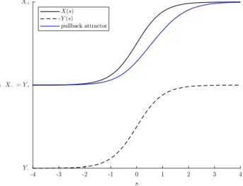
5.5 An illustration of a stable path and trajectories for Example 5.2.11. Three different pullback attractors toX−=0.90 are plotted, with differing values ofr. Whenris smaller, the pullback attractor stays closer to the path. . . 89
5.6 An illustration of paths and trajectories for Example 5.3.2. When r = 0.2, the pullback attractor toX−endpoint tracks the path (s,X(s)), but whenr =0.5, the pullback attractor does not endpoint track, showing that there is rate-induced tipping. . . 91
5.7 An illustration of paths and a trajectory for Example 5.3.4. The two red dashed curves together form the boundary of a connected component of the basin of attraction for the stable path (s,X(s)). Even though (s,X(s)) is forward basin stable, the pullback attractor toX−does not endpoint track the path whenr =2. . . 92
5.9 HereR=0.9,φ=1, p=6, anda=0.5. These parameter values lead to three fixed points: X+,Y+, andZ+(listed in order from largest to smallest norm). Y+is a saddle node, whose 1-dimensional stable manifold (plotted in blue) forms the boundary of the basins of attraction of the stable fixed pointsX+(white) andZ+(gray). The pointX−≈(2.9698,5.0274) is the largest-norm fixed point whena=4.5 and the other parameter values remain the same; notice
LIST OF TABLES
4.1 Categories of tropical cyclones based on their windspeeds, according to [2] and [3]. . . 56 4.2 Definitions of variables and parameters in (4.1). Values and units with an asterisk∗are given
CHAPTER 1 Introduction
Rate-induced tipping is a drastic change in the behavior of a system due to quickly-changing parameters. Imagine trying to pull a tablecloth out from under a set of dishes on a table. If the tablecloth is pulled slowly, it will carry all the dishes with it, but if the tablecloth is pulled quickly enough, the dishes will be left behind on the table. Here we get two distinct outcomes: the dishes come with the tablecloth or they get left behind. The deciding factor between these outcomes is not howfarthe tablecloth moves, but howfast. Likewise, with rate-induced tipping (R-tipping), the behavior of solutions is determined not by howmuchthe parameters change, but howquickly. This kind of tipping has been observed in a variety of physical applications, such as the rise of temperatures in peatlands [32].
There are different reasons that tipping can happen in a system. In particular [7] describes three types of tipping: bifurcation-, noise-, and rate-induced. Bifurcation-induced tipping happens due to a bifurcation in the system (say, the annihilation of a stable fixed point) and is the result of parameters changing toomuch. With rate-induced tipping, there is no such bifurcation in the system to explain the sudden change in behavior. Noise-induced tipping happens as a result of noise in the system, which rate-induced tipping does not require, although there can be interplay between the two phenomena, as studied in [26]. We will focus solely on rate-induced tipping and ensure that other types of tipping are not at play by avoiding stochastic systems and parameter changes that lead to bifurcations.
Most of the literature on rate-induced tipping is in the context of continuous-time dynamical systems (flows), but we will study R-tipping in discrete-time dynamical systems (maps) as well. Drawing from [6], we will give a precise definition of rate-induced tipping in flows in this chapter and then make appropriate adaptations for the context of maps in Chapter 5.
Suppose we have an autonomous dynamical system
˙
wherex∈UforU ⊂R`open,λ∈Rm, f ∈C2(U×
Rm,R`), and ˙xmeans derivative with respect to time, dxdt.
We want to allow the parameterλto vary from one value to another over time, so we replace it with aC2
functionΛ:R→Rmsatisfying
lim
s→±∞Λ(s)=λ± lim
s→±∞Λ 0(
s)=0
(1.2)
for someλ±∈Rm. In [6], such a function is called aparameter shift. The set of all parameter shifts satisfying
(1.2) for a givenλ±is denoted byP(λ−, λ+). To allow the parameter to shift at different rates, we introduce
r>0 and obtain a nonautonomous system
˙
x= f(x,Λ(rt)). (1.3)
The value r can be thought of as therateat which Λ changes. Whenr is small, the parameter shift is gradual, and in fact ifr = 0, then (1.3) reduces to (1.1) whereλ = Λ(0). Whenris large, the parameter shift approximates the step function which steps fromλ−toλ+att=0. We are interested in comparing the behavior of solutions to (1.3) for different values ofr.
We can also view (1.3) as an autonomous system of one higher dimension by introducing the variable
s=rtand rewriting (1.3) as
˙
s=r
˙
x= f(x,Λ(s)).
(1.4)
In what follows, it will be helpful to have different notation for the flow of (1.1) and the flow of (1.3). So, we will use the dot notation
x·λ0t
to denote a trajectory of (1.1) withλ=λ0, whilex(t) will denote a trajectory in (1.3).
For a square matrix M, letσ(M) denote the spectrum ofM. Then we define apathas follows:
Definition 1.0.1. LetΛ∈ P(λ−, λ+). Suppose that for alls∈R,X(s) is a fixed point of (1.1) withλ= Λ(s) such that (s,X(s)) is a connected curve. Suppose also that this extends to the limits as s → ±∞, so
1. astable pathif max{Reσ(Dxf(X(s),Λ(s)))}<0 (that is,X(s) is an attracting fixed point of (1.1) with λ= Λ(s)) for alls∈R∪ {±∞};
2. anunstable pathif max{Reσ(Dxf(X(s),Λ(s)))}>0 (that is,X(s) is an unstable fixed point of (1.1) withλ= Λ(s)) for alls∈R∪ {±∞}.
Paths act as a guideline against which we can compare solutions of (1.3).
Definition 1.0.2. SupposeΛ∈ P(λ−, λ+) gives rise to a stable path (s,X(s)) in (1.3) withX±=lims→±∞X(s). As shown in Theorem 2.2 of [6], there is a unique trajectory xr(t) of (1.3) such that limt→−∞xr(t)= X−, which is the local pullback attractorto X−. If limt→∞xr(t) = X+, then we say thatxr(t)endpoint tracks ortracksthe path (s,X(s)). By Lemma 2.3 of [6],xr(t) endpoint tracks (s,X(s)) for all sufficiently small r >0, but if limt→∞xr(t), X+for somer>0, then there has beenrate-induced tippingaway fromX−. If limt→∞xr(t)=Y+for someY+,X+, then we say there has been rate-induced tipping fromX−toY+.
Our focus is on giving conditions for systems and parameter shifts in which rate-induced tipping will happen for some value ofr >0. Some others who study rate-induced tipping are interested in finding the
critical rate r0>0, which is the smallest value ofrfor whichxr(t) does not endpoint track a path. Although
this is interesting and worthwhile, this will not be our focus here.
The authors of [6] explore conditions under which rate-induced tipping can be expected to happen (or not happen) in systems of the form (1.3) where`=1. We will use their work as a springboard to study both rate-induced tipping in flows when` >1 in Chapter 2 and rate-induced tipping in maps in Chapter 5. It will be helpful to restate the following definition and result from [6] that we will reference throughout.
Definition 1.0.3. Let x∈R`be an attracting fixed point of (1.1) for a given value ofλ. ThenB(x, λ) is the
basin of attraction forxin (1.1). That is,
B(x, λ)=
y∈R` : lim
t→∞y·λt= x
.
A stable path (s,X(s)) isforward basin stableif
{X(u) :u<s} ⊂B(X(s),Λ(s))
The following theorem follows from the proof of Theorem 3.2 of [6] and establishes conditions under which we can expect rate-induced tipping to occur (or not occur) in a system of the form (1.3) when`=1: Theorem 1.0.4. Suppose Λ ∈ P(λ−, λ+) gives rise to a stable path (s,X(s)) in (1.3) with ` = 1 and X±=lims→±∞X(s).
1. If(s,X(s))is forward basin stable, there can be no R-tipping away from X−for thisΛ.
2. If there is another stable path(s,Y(s))with Y±=lims→±∞Y(s)such that Y+, X+and there are u<v such that X(u) ∈ B(Y(v),Λ(v)), then(s,X(s))is not forward basin stable. Furthermore, there is a parameter shiftΛ˜ (a time-reparameterization ofΛ) that gives rise to stable paths(s,X˜(s))and(s,Y˜(s))
where
X±= lim
s→±∞X(s)= s→±∞lim ˜
X(s)
Y±= lim
s→±∞Y(s)=s→±∞lim ˜
Y(s)
(1.5)
such that there is R-tipping away from X−to Y+for thisΛ˜ and some r>0.
3. If there is a Y+,X+such that Y+is an attracting equilibrium of (1.1)forλ=λ+and X−∈B(Y+, λ+), then(s,X(s))is not forward basin stable and there is R-tipping away from X−to Y+for thisΛfor all
sufficiently large r>0.
CHAPTER 2
Rate-induced Tipping in Multi-dimensional Flows1
In this chapter we will study rate-induced tipping in systems of the form (1.3) when` >1. In particular, we want to know the relationship between forward basin stability and R-tipping. We know from Theorem 1.0.4 that forward basin stability prevents R-tipping and also that certain kinds of forward basin instability lead to R-tipping when` =1. As we will see in Section 2.1, the same kinds of forward basin instability guarantee R-tipping for` >1 as well. However, as we will show in Section 2.2, forward basin stability is not a strong enough condition to prevent R-tipping when` >1. Instead, we propose a different condition, forward inflowing stability, which is enough to prevent R-tipping in systems of any dimension. Although this condition is natural, forward inflowing stability can be difficult to verify in general concrete examples, so in Section 2.3 we will narrow our focus tomonotone systems. Monotone systems are a class for which forward inflowing stability is implied by an easily verifiable condition, and we will see how the additional structure of these systems makes predicting the possibility of R-tipping straightforward as in 1-dimensional systems. 2.1 Conditions to Guarantee R-Tipping
In this section we will prove that statements 2 and 3 of Theorem 1.0.4 generalize to multi-dimensional systems. First, we must establish some lemmas that will be used in the proof of these results.
This first lemma deals with the initial behavior of the pullback attractor toX−.
Lemma 2.1.1. SupposeΛ∈ P(λ−, λ+)gives rise to a stable path(s,X(s))in(1.3)with X−=lims→−∞X(s).
Let xr(t)be the pullback attractor to X−, and letk · kbe any vector norm onR`. Givenε >0, there exists an S >0such thatkxr(t)−X−k ≤εwhen rt<−S .
The proof closely follows the proof of Theorem 2.2 in [6]:
1This chapter is adapted from an article in the Journal of Dynamics and Differential Equations. The original citation is as follows: C.
Kiers and C. K. R. T. Jones. On conditions for rate-induced tipping in multi-dimensional dynamical systems.J. Dynam. Differential
Proof. Let us assume for the sake of simplicity thatX−=0. Define
ω(ε) :=sup{kDxf(x,Λ(s))−Dxf(0,Λ(s))k:s∈R,kxk ≤ε} δ(S) :=max
(
sup
s<−S
kf(0,Λ(s))k,sup
s<−S
kDxf(0,Λ(s))−Dxf(0, λ−)k
)
,
wherek · kalso denotes the induced matrix norm. Note thatω(ε)→0 asε→0 andδ(S)→0 asS → ∞. By the linear stability ofX−, the eigenvalues ofA:=Dxf(0, λ−) have negative real parts, so there areK>0
andα >0 such that e
tA
≤ Ke
−αt fort≥0 (see Lemma 3.3.19 of [15]). Now seth(x,s)= f(x,Λ(s))−Ax
so that
˙
x= Ax+h(x,s) (2.1)
Then
Dxh(x,s)=Dxf(x,Λ(s))−A
=
Dxf(x,Λ(s))−Dxf(0,Λ(s))+
Dxf(0,Λ(s))−Dxf(0, λ−)
Therefore, ifs<−S, we have
kh(0,s)k ≤δ(S), kDxh(x,s)k ≤ω(kxk)+δ(S).
Consider the inequalities
4Kα−1ω(ε)≤1 2Kα−1δ(S)≤ε 4Kα−1δ(S)≤1,
(2.2)
forε,S >0. If we chooseεsufficiently small, we can find someS0>0 to satisfy (2.2). Now, we know that
δ(S)→0 asS → ∞, so there is anS1 >0 such thatS ≥S1implies thatδ(S)≤δ(S0). Then ifS ≥S1, (2.2) is satisfied.
asrt<−S1.
LetPbe space of continuous functions x(t) defined fort <−S1
r such thatkx(t)k ≤ ε. We define ˆxfor x∈ Pby
ˆ
x(t)=
Z t
−∞
e(t−u)Ah(x(u),ru)du.
Then ifx∈ P, ˆx=xif and only ifx(t) is a solution of (2.1). Also,
kxˆ(t)k ≤ε,
sox7→xˆis a map fromPto itself. Furthermore, ifx1,x2∈ P, then
sup
t<−S1/r
kˆx1−xˆ2k ≤ 1 2t<−supS1/r
kx1−x2k.
Thus,x7→xˆis a contraction mapping onP, so there is a uniquex(t)∈ Psuch thatx(t)=xˆ(t). Thisx(t) is a solution to (2.1) and satisfieskx(t)k ≤εfor allt<−S1/r. Thisx(t) must be the pullback attractor toX−=0, since the pullback attractor is the only trajectory of (1.3) that stays within a small neighborhood ofX−for all
backward time. (See Theorem 2.2 of [6].)
Next, we discuss the end behavior of trajectories of (1.3). The purpose of Lemmas 2.1.2 - 2.1.5 is to show that ifX+is an attracting fixed point of (1.1) withλ=λ+, then any trajectory of (1.3) that is in a compact subset ofB(X+, λ+) for large enoughtwill converge toX+.
In autonomous systems, the omega limit set of a point x is defined to be ω(x) = {y : x · tn → yfor sometn → ∞}. Omega limit sets have the property that if z ∈ ω(y) and y ∈ ω(x), then z ∈ ω(x)
(see Section 4.1 of [28]). This next lemma states that, in a certain sense, this property holds in nonautonomous systems like (1.3).
Lemma 2.1.2. LetΛ∈ P(λ−, λ+). Suppose y·λ+sn→z for some{sn} → ∞. If x(t)is a trajectory of (1.3) such that x(tn)→y for some{tn} → ∞, then there exist{un} → ∞for which x(un)→z.
Proof. Fixr > 0. Letk · kdenote any norm onR`. For eachn ∈ N, there exists some Nn ∈ Nsuch that m≥Nnimpliesky·λ+ sm−zk< 1n. (Ifn≥ 2, chooseNn >Nn−1.) SinceΛ(rt)→λ+ast→ ∞, there exists
someTn>0 andδn>0 such that ifkx(t)−yk< δnandt>Tn, thenkx(t+sNn)−y·λ+sNnk< 1
n. There exists
Now, setun =sNn +tMn. Then,
kx(un)−zk=kx(sNn+tMn)−zk
≤ kx(sNn+tMn)−y·λ+ sNnk+ky·λ+ sNn−zk
< 1
n +
1
n
= 2
n
Therefore,x(un)→zasn→ ∞.
If pis an attracting fixed point of an autonomous system, there are arbitrarily small forward invariant neighborhoods ofp. (This is follows from the Stable Manifold Theorem; see Theorem 2.1 in Chapter 10 of [27].) This next lemma states that a similar statement is true for the limit of a stable path in (1.3).
Lemma 2.1.3. SupposeΛ∈ P(λ−, λ+)gives rise to a stable path(s,X(s))in(1.3)with X+=lims→∞X(s).
Then there exists a normk · kxonR`such that for all sufficiently smallε >0, there exists an S >0such that ifkx(T)−X+kx ≤εfor rT >S , thenkx(t)−X+kx≤εfor all t≥T .
Proof. Let us assume for the sake of simplicity thatX+=0 andλ+=0. Since (X+, λ+)=(0,0) is attracting, all eigenvalues ofA:=Dxf(0,0) have negative real part, so there is somek > 0 such that Re(µ)<−kfor every eigenvalueµofA. We can choose an inner producth,ionUsuch thathAx,xi ≤ −khx,xifor allx∈U
(see the lemma in Chapter 7, Section 1 of [16]). This defines a normkx0kx =hx0,x0i1/2. Letk · kλ be any
vector norm onRm. By Taylor’s formula in several variables we can write
f(x0, λ0)= Ax0+α(x0, λ0)+β(x0),
where kα(x0, λ0)kx ≤ γ(x0, λ0)kλ0kλ for a positive continuousγ, andkβ(x0)kx ≤ δ(x0)kx0kx, where δ is
positive, continuous andδ(x0)→0 asx0 →0. Then we can write (1.3) as
dx
Then
d dt
kx0k2x
=2
*
dx0 dt ,x0
+
=2hAx0,x0i+2hα(x0,Λ(rt)),x0i+2hβ(x0),x0i
≤ −2khx0,x0i+2kα(x0,Λ(rt))kxkx0kx+2kβ(x0)kxkx0kx
≤ −2kkx0k2x+2γ(x0,Λ(rt))kΛ(rt)kλkx0kx+2δ(x0)kx0k2x
=2kx0k2x −k+2γ(x0,Λ(rt))
kΛ(rt)kλ kx0kx +
δ(x0)
!
Chooseε >0 such that ifkx0kx≤ε,δ(x0)< k2. Then chooseS >0 such that ifrt>S,kΛ(rt)kλ < 4Mkε where M>supkx0kx≤ε,λ∈[λ−,λ+]γ(x0, λ). Thus, ifkx0kx =εandrt>S,
d
dt(kx0kx)
2<2ε2 −k+2γ(x
0,Λ(rt)) kε
4Mε
!
+ k 2
!
<2ε2 −k+ k
2+
k
2
!
=0
Therefore, the vector field of (1.3) points into{y ∈ R` : kykx ≤ ε}on its boundary whenrt > S, so for a
givenr>0 ifx(t) is a solution of (1.3) andkx(T)−X+kx ≤εfor someT >S/r, thenkx(t)−X+kx≤εfor all
t≥T.
Ifpis an attracting fixed point of an autonomous system, then by the Stable Manifold Theorem there is a neighborhoodVof psuch that all trajectories with initial conditions inVconverge to p. This next lemma shows that a similar thing is true for the limit of a stable path in (1.3).
Lemma 2.1.4. SupposeΛ∈ P(λ−, λ+)gives rise to a stable path(s,X(s))in(1.3)with X+=lims→∞X(s),
and let k · kx be the norm on R` from Lemma 2.1.3. There exists an ε > 0 and an S > 0 such that if
kx(t)−X+kx < εfor rt>S , then x(t)→X+as t→ ∞.
Proof. Pick anε > 0 sufficiently small for Lemma 2.1.3. Makeεsmaller if necessary so thatBε(X+) ⊂
B(X+, λ+). Then by Lemma 2.1.3, there exists an S > 0 such that if x(T) ∈ Bε(X+) forrT > S, then
there exists a sequence{un} → ∞such thatx(un)→X+.
Now pick anyδ∈(0, ε). Then by Lemma 2.1.3, there exists someSδ > 0 such that ifx(T)∈ Bδ(X+) forrT > Sδ, then x(t) ∈ Bδ(X+) for allt≥ T. By the previous paragraph, there is aunδ > Sδ/r such that x(unδ)∈Bδ(X+). Therefore,x(t)∈Bδ(X+) for allt≥unδ. Hencex(t)→X+ast→ ∞.
Using the preceding lemmas we can conclude the following:
Lemma 2.1.5. SupposeΛ∈ P(λ−, λ+)gives rise to a stable path(s,X(s))in(1.3)with X+=lims→∞X(s).
Let K⊂B(X+, λ+)be compact. Then there exists an S >0such that if x(T)∈K for rT >S , then x(t)→X+ as t→ ∞.
Proof. Letk · kxbe the norm onR`from Lemma 2.1.4. By Lemma 2.1.4, there is anε >0 and anS1> 0
such that ifkx(t)−X+kx≤εforrt>S1, thenx(t)→X+ast→ ∞. SinceK⊂B(X+, λ+) is compact, there is someT0 >0 such thaty·λ+t∈Bε/2(X+) for anyy∈Kandt≥ T0. Also, there is someS2 >0 such that if x(T)=y0∈KforrT >S2, thenkx(T +T0)−y0·λ+T0kx < ε/2 for anyy0∈K.
TakeS =max{S1,S2}. Then, supposex(T)∈KforrT >S. Ifx(T)=y0, then
kx(T +T0)−X+kx ≤ kx(T +T0)−y0·λ+T0kx+ky0·λ+T0−X+kx
< ε/2+ε/2 =ε
Therefore,x(t)→X+ast→ ∞.
Now we are ready to prove the generalization of statements 2 and 3 of Theorem 1.0.4:
Theorem 2.1.6. Suppose Λ ∈ P(λ−, λ+) gives rise to a stable path (s,X(s)) in (1.3) with ` ∈ N and X±=lims→±∞X(s).
where
X±= lim
s→±∞X(s)= s→±∞lim ˜
X(s)
Y±= lim
s→±∞Y(s)= s→±∞lim ˜
Y(s)
(2.3)
such that there is R-tipping away from X−to Y+for thisΛ˜ and some r>0.
2. If there is a Y+,X+such that Y+is an attracting equilibrium of (1.1)forλ=λ+and X−∈B(Y+, λ+), then(s,X(s))is not forward basin stable and there is R-tipping away from X−to Y+for thisΛfor all
sufficiently large r>0.
Proof. We will prove statement 1 first. Based on the assumptions, it is clear that (s,X(s)) is not forward basin stable. We will construct a parameter shift ˜Λthat gives R-tipping away fromX−. Letk · kbe any norm onR`.
Pickε >0 such thatK= Bε(X(u))⊂B(Y(v),Λ(v)). By Lemma 2.3 of [6], there is anr0 >0 such that for all
r∈(0,r0),kxr(s/r)−X(s)k< ε/2 for alls∈R. Likewise, there exists anr1 >0 such that for allr∈(0,r1), if
xr(v/r)∈K, thenxr(t)→Y+ast→ ∞. Now fixr∈(0,min{r0,r1}).
We will construct a reparametrization
˜
Λ(s) := Λ(σ(s))
using a monotonic increasingσ∈C2(R,R) that increases rapidly fromσ(s)=utoσ(s)=vbut increases
slowly otherwise. In particular, for anyM>1 andη >0 we choose a smooth monotonic functionσ(s) such that
σ(s)= s for s<u
1≤ dsdσ(s)≤ M for u≤σ(s)≤u+η d
dsσ(s)= M for u+η < σ(s)<v−η
1≤ dsdσ(s)≤ M for v−η≤σ(s)≤v, and
d
dsσ(s)=1 for σ(s)>v
(2.4)
Let ˜xr(t) denote the pullback attractor to X−with parameter shift ˜Λ. By construction, we know that ˜
xr(u/r)∈Bε/2(X(u)). By choosingM>1 sufficiently large andη >0 sufficiently small, we can guarantee
Now we will prove statement 2. Pickε >0 such thatB3ε(X−)⊂B(Y+, λ+). By Lemma 2.1.1, there is an S1>0 such that the pullback attractorxr(t) toX−satisfiesxr(t)∈Bε(X−) ifrt<−S1. By Lemma 2.1.5, there
is someS2 >0 such that ifxr(t)∈B2ε(X−) forrt>S2thenxr(t)→Y+ast→ ∞. TakeS =max{S1,S2}. By continuity, there is some M> 0 such thatkf(x, λ)k< Mfor all x∈ B2ε(X−) andλ∈[λ−, λ+]. Pick
any
r>2MS ε .
Suppose for the sake of contradiction that xr(S/r) < B2ε(X−). We knowxr(−S/r) ∈ Bε(X−), so let s0 =
inf{s∈(−S,S] :xr(s/r)<B2ε(X−)}. Then in facts0is a minimum ands0>−S. By Theorem 9.19 of [29],
kxr(−S/r)−xr(s0/r)k ≤M
−S
r − s0 r
< M2S r < ε.
Because xr(−S/r) ∈ Bε(X−), this implies that xr(s0/r) ∈ B2ε(X−), which is a contradiction. Therefore,
xr(S/r)∈B2ε(X−). As shown above, this implies thatxr(t)→Y+ast→ ∞. Hence, there is R-tipping away
fromX−toY+for all sufficiently larger>0.
Example 2.1.7. We can apply Theorem 2.1.6 to the Lorenz equations:
˙
x=σ(y−x) ˙
y=x(ρ−z)−y
˙
z=xy−βz
(2.5)
The traditional parameter choices for demonstrating chaos in (2.5) areσ=10,β=8/3, andρ=28. However, we are not interested in demonstrating chaos but in showing R-tipping in a system with attracting fixed points. So, as in [30], we will fixσ =10 andβ=8/3, but we will allowρto vary with time. The corresponding augmented system for (2.5) is
˙
s=r
˙
x=10(y−x) ˙
y=x(P(s)−z)−y
˙
z=xy−8 3z
forr >0 andPa parameter shift. We will allowρto monotonically increase from 15 to 23, soρ−=15 and ρ+=23. As explained in [9] and [30], in this parameter regime there are three equilibria, one at the origin and the other two
C1 =
p
8/3(ρ−1),p8/3(ρ−1), ρ−1
C2 =
−p8/3(ρ−1),−p8/3(ρ−1), ρ−1.
BothC1,2are attracting, and the origin is a saddle point. There are heteroclinic connections from the origin to C1,2, and there are periodic orbits aroundC1,2. There is no chaotic attractor for these values ofρ.
(2.6) has two stable paths (s,C1(s)) and (s,C2(s)) with
C1(s)=
p
8/3(P(s)−1), p8/3(P(s)−1),P(s)−1
C2(s)=−p8/3(P(s)−1),−p8/3(P(s)−1),P(s)−1
andC1,2±= lims→±∞C1,2(s). We will consider the possibility of R-tipping away fromC1−. From Figure
2.1, we see that (s,C1(s)) is not forward basin stable becauseC1(u)∈B(C2(v),P(v)) whereP(u)=15.1 and P(v)=22.9. Therefore, according to Theorem 2.1.6, we can expect R-tipping for some choices ofPand
r>0. Indeed if we choose
P(s)=4 tanh(s)+19
then for some values ofr>0 the pullback attractor toC1−tracks (s,C1(s)) and for some values ofr>0 it
tips toC2+(see Figure 2.2).
2.2 Forward Basin Stability and Forward Inflowing Stability
Now that we have successfully generalized statements 2 and 3 of Theorem 1.0.4, we will turn our attention to statement 1, which says that if a path is forward basin stable in a 1-dimensional system, then there will be no R-tipping away from that path. However, as the next example shows, forward basin stability is not enough to prevent R-tipping in systems where` >1.
Figure 2.1: The solution to (2.5) withρ = 22.9 and initial condition (√8/3(14.1),√8/3(14.1),14.1) con-verges to a point on (s,C2(s)), indicating that (s,C1(s)) is not forward basin stable.
0
15 -10
5 10
10 -5
15 20
0 5
25 30
5 0
10 -5
-10 15
0
-20 30
10
20 20
-10 30
10 0
40
0
10 -10
20 -20
Figure 2.2: The blue/green curves mark the positions ofC1,2(s), with the blue corresponding to smaller values
ofs. The red curve is the pullback attractor toC1−. Whenr =13 the trajectory endpoint tracks (s,C1(s)), but
Figure 2.3: Phase portrait for system (2.7). The homoclinic orbits at (λ,0) are shown in black.
of [28]):
˙
x=−y
˙
y=−(x−λ)+2(x−λ)3−y((x−λ)2−(x−λ)4−y2).
(2.7)
Then (2.7) has fixed points at (λ,0) and
λ± √1
2,0
. There are two homoclinic orbits at (λ,0) defined by the curvesy=±p(x−λ)2−(x−λ)4. Bothλ± √1
2,0
are attracting, and their basins of attraction are the regions inside the corresponding homoclinic orbits. See Figure 2.3.
Then we will letλchange with time at a rater>0 by settingλ= Λ(s) ands=rt:
˙
s=r
˙
x=−y
˙
y=−(x−Λ(s))+2(x−Λ(s))3−y((x−Λ(s))2−(x−Λ(s))4−y2).
(2.8)
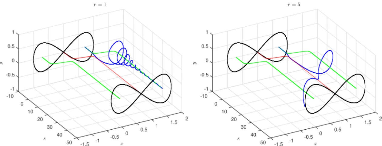
ForΛwe will takeΛ(s)= 1340(1+tanh(s)) so thatλ−=0 andλ+=0.65< √1
2. LetX(s)=
Λ(s)+ √1
2,0
. Then X− =
1
√
2,0
andX+ =
1
√
2+ 13 20,0
. Because 0 < Λ(s) < √1
2 for all s, the stable path (s,X(s)) is
forward basin stable. Nevertheless, R-tipping can occur away fromX−. See Figure 2.4.
-1 -10
0 -0.5
10 0
2 20
1.5 1 30
0.5
0.5 0
40 -0.5
-1 1
50 -1.5
-1 -10
0 -0.5
10 0
2 20
1.5 1 30
0.5
0.5 0
40 -0.5
-1 1
50 -1.5
Figure 2.4: Phase portraits for (2.8) for two different values ofr. Stable paths are shown green, and the unstable path in red. The black loops show the positions of the homoclinic orbits in (2.7) whens=−10 and 50. The blue curve is the pullback attractor toX−. Whenr=1 the pullback attractor endpoint tracks (s,X(s)), but whenr=5 it diverges to infinity.
system is that a pointxmight be in the basin of attraction of a fixed pointp, but the velocity vector atxmay not point towardp. The more dimensions there are in a system, the more directions there are to move, so in a sense this makes R-tipping more likely to happen. Although Example 2.2.1 is an example of a 2-dimensional system, it would not be difficult to construct a system of higher dimension in which there can be R-tipping away from a path that is forward basin stable.
Therefore, since forward basin stability is not enough to prevent R-tipping in systems of dimension greater than 1, we want to find a different condition that is sufficient to prevent R-tipping. We propose a condition calledforward inflowing stabilitywhich guarantees that R-tipping cannot happen away from a stable path.
Definition 2.2.2. SupposeΛ∈ P(λ−, λ+) gives rise to a stable path (s,X(s)) in (1.3) withX±=lims→±∞X(s). Then (s,X(s)) isforward inflowing stableif for eachs∈Rthere exist compact setsK(s)⊂Uwith nonempty interior satisfying
(P1) ifs1< s2, thenK(s1)⊂ K(s2);
(P2) ifx∈∂K(s), then∃t0 >0 such thatx·Λ(s)t∈IntK(s) for allt∈(0,t0);
(P3) X±∈IntK±whereK−=Ts∈RK(s) andK+= S
s∈RK(s); and
(P4) K+⊂B(X+, λ+) is compact.
Just as the notion of forward basin stability compares the positions of equilibria along a path to basins of attraction later on in the path, forward inflowing stability compares the positions of equilibria along the path to forward invariant sets (sets for which solutions “flow in”) later on down the path.
Theorem 2.2.3. SupposeΛ∈ P(λ−, λ+)gives rise to a forward inflowing stable path(s,X(s))in(1.3)with X±=lims→±∞X(s). Then there will not be R-tipping away from X−.
Proof. Fixr>0. By forward inflowing stability, there exist setsK(s) satisfying the requirements of Definition 2.2.2. SetK =∪s∈R(s,K(s)). By (P2) if we pick a pointxon the boundary ofKwhen s =s0, then there
exists at0 > 0 such that x·Λ(s0)t∈ IntK(s0) for allt∈ (0,t0). SinceK(s0) ⊂ K(s) ifs0 < sby (P1) and
ds
dt =r>0, there is somet1>0 such thatx(t)∈IntKfor allt∈(0,t1), where x(t) is the solution with initial
conditionx(0)=xin (1.4). Therefore,Kis forward invariant under the flow of (1.4).
Let xr(t) be the pullback attractor toX−. BecauseX−∈IntK−andK− =Ts∈RK(s) by (P3), there is a T ∈Rsuch thatxr(t)∈K(rt) for allt<T. SinceKis forward invariant, this implies thatxr(t)∈K(rt) for all
t∈R. In particular,xr(t)∈K+for allt∈R.
We know K+ ⊂ B(X+, λ+) is compact by (P4). By Lemma 2.1.5 this impliesxr(t) → X+ ast → ∞. Therefore,xr(t) endpoint tracks the stable path (s,X(s)) regardless ofr>0, so there is no R-tipping.
Example 2.2.4. SupposeΛ∈ P(λ−, λ+) gives rise to the paths in Figure 2.5. Let (s,X(s)) be the stable path that is defined for alls-values. For each value of s, letK(s) be the closed interval between the two red curves. Based on what is shown in the figure,{K(s)} satisfies the requirements in Definition 2.2.2, which shows that (s,X(s)) is forward inflowing stable. The setK=∪s∈R(s,K(s)) forms a “tube” around the stable path
(s,X(s)) that is forward invariant under (1.4). As shown in Theorem 2.2.3, the pullback attractor toX−is always contained inK. There can be no R-tipping away fromX−for this reason.
Figure 2.5: (s,X(s)) is forward inflowing stable but not forward basin stable.
Figure 2.6: (s,X(s)) is forward basin stable but not forward inflowing stable.
Note that in multi-dimensional systems forward basin stability cannot imply forward inflowing stability, as forward inflowing stability prevents R-tipping, but forward basin stability does not.
2.3 Monotone Systems
We will now focus our attention on rate-induced tipping in a special class of systems called monotone systems. The benefit of monotone systems is that their extra structure enables us in Proposition 2.3.2 to prove when rate-induced tipping can happen without having to calculate the basins of attraction of the equilibria (which can be chaotic in systems of dimension 3 or more, such as in Lorenz ‘63–see [9]). Likewise, in Proposition 2.3.3 we will be able to prove when rate-induced tipping cannot happen, since inflowing stability is easier to determine in these systems.
ordering on the real numbers. To extend this notion to systems of dimension higher than 1, we need to define an ordering on multi-dimensional spaces. We will use the following partial ordering onR`:
Suppose x=(x1, . . . ,x`),y=(y1, . . . ,y`)∈R`. Then
x≤y ⇐⇒ xi≤yifor alli x<y ⇐⇒ x≤yandx,y xy ⇐⇒ xi<yifor alli.
IfK,L⊂R`are sets, we will writeK Lto mean xyfor all x∈Kandy∈L. Furthermore, a setKis
p-convexif for everyx,y∈Ksatisfyingx≤y, the line segment joining them also belongs toK.
Intuitively, a monotone system is a dynamical system that preserves this partial ordering. More specifically, a system of the form (1.1) ismonotoneif x·λt≤ y·λtwheneverx ≤ y ∈R`andt≥ 0. Section 3 of [17] demonstrates that ifUis p-convex, then
˙ x1 · · · ˙ x` =
f1(x1, . . . ,x`)
· · ·
f`(x1, . . . ,x`)
is monotone if and only if
∂fi
∂xj
≥0∀i, j. (2.9)
We begin by proving a lemma about forward invariant sets in monotone systems which we will use later to prove a result about R-tipping in monotone systems:
Lemma 2.3.1. Suppose(1.1)is a monotone system and U is p-convex. For any p∈U, define K1(p)={x∈
U:x≤ p}and K2(p)={x∈U:x≥ p}. If fi(p, λ)<0( fi(p, λ)>0) for all i, then the vector field f points into K1(K2) on the boundary of K1(K2), so K1(K2) is forward invariant.
Proof. Since (1.1) is monotone andUis p-convex, we know that ∂fi
∂xj ≥0 for alli, j.
The result is trivial if`=1, so we will assume`≥2. We will prove the statement forK2; the proof for
K1is similar.
Y(s)
Z(s)
Figure 2.7: IfZ(s) is chosen as in Proposition 2.3.2, then the boxK2(Z(s)) (shown in gray) has the flow of (1.1) withλ= Λ(s) pointing in on all sides along its boundary.
ofK2. The linelthroughyandpcan be parametrized byτas
l(τ)=((y1−p1)τ+p1,(y2−p2)τ+p2, . . . ,(y`− p`)τ+p`),
sol(0)= pandl(1)=y. We need to show that ˙xi >0 aty, or fi(l(1), λ)>0, for allisuch thatyi= pi. We know that fi(l(0), λ)>0, so it will suffice if ∂τ∂ fi(l(τ), λ)≥0. This is indeed the case because
∂
∂τfi(l(τ), λ)=Dxfi(l(τ), λ)·l0(τ) = ∂fi
∂x1
, ∂fi
∂x2
, . . . , ∂fi
∂x`
!
(l(τ), λ)·(y1−p1,y2−p2, . . . ,y`− p`)
≥0
because each ∂fi
∂xj(l(τ), λ)(yj−pj)≥0.
Using Lemma 2.3.1 we can establish the following result about when there will be R-tipping in monotone systems:
Proposition 2.3.2. SupposeΛ∈ P(λ−, λ+)gives rise to a stable path(s,X(s))and an unstable path(s,Y(s))
(including in the limits) Dxf(Y(s),Λ(s))has a positive eigenvalue whose associated eigenvector has all positive components.
1. If X(s) Y(s)(resp. Y(s) X(s)) for all s ∈ R, including in the limits as s → ±∞, and there are u < v such that Y(v) X(u)(resp. X(u) Y(v)), then there is a parameter shiftΛ˜ (a time-reparameterization ofΛ) such that there is R-tipping away from X−for thisΛ˜ for some r>0.
2. If X(s) Y(s)(resp. Y(s)X(s)) for all s ∈R, including in the limits as s→ ±∞, and Y+ X−
(resp. X−Y+), then there will be R-tipping away from X−for thisΛfor all sufficiently large r>0.
Proof. We will prove statement 1. The proof of statement 2 is similar but does not require any time-reparameterization ofΛ. SupposeX(s)Y(s) for alls∈Rincluding in the limits and thatY(v)X(u). Let
xr(t) denote the pullback attractor toX−.
Letk · kbe any vector norm onR`, and pickε >0 such that{Y(v)} Bε(X(u)). By Lemma 2.3 of [6], there is anr0>0 such that for all 0<r <r0,kxr(s/r)−X(s)k< ε/2 for alls∈R.
For anys∈R, sinceDxf(Y(s),Λ(s)) has a positive real eigenvalue with an eigenvector that has all positive
components, by the Stable Manifold Theorem (see [24]) there is a pointZ(s) such that{Y(s)} {Z(s)·Λ(s)t}t≤0
and fi(Z(s),Λ(s))>0 for alli. Then defineK2(Z(s))={x∈U :x≥Z(s)}. By Lemma 2.3.1, the vector field f(x,Λ(s)) is pointing in on all sides along the boundary ofK2(Z(s)). See Figure 2.7 for an illustration.
BecauseZ(s) can be chosen to be arbitrarily close toY(s), we may also assume that thatZ(v) satisfies {Z(v)} Bε(X(u)) and thatZ(s) varies continuously ins.
Because the system converges as s→ ∞, there is anS0>vsuch that the flow of the autonomous system
(1.1) withλ= Λ(s) points in along the boundary ofK2(Z(S0)) for everys≥S0andX+<K2(Z(S0)). Then K2(Z(S0))×[S0,∞) is forward invariant under the flow of (1.4) for anyr>0. Additionally, we can choose
r1 >0 sufficiently small so that
[
s∈[v,S0]
(s,K2(Z(s)))
is forward invariant under the flow of (1.4). Now fixr∈(0,min{r0,r1}). As in the proof of Theorem 2.1.6, we can construct a reparametrization
˜
Λ(s) := Λ(σ(s))
increases slowly otherwise. In particular, for anyM>1 andη >0 we choose a smooth monotonic function σ(s) that satisfies (2.4).
Let ˜xr(t) denote the pullback attractor to X−with parameter shift ˜Λ. By construction, we know that ˜
xr(u/r)∈Bε/2(X(u)). By choosingM>1 sufficiently large andη >0 sufficiently small, we can guarantee
that ˜xr(v/r) ∈ Bε(X(u)) ⊂ K2(Z(v)). This implies that ˜xr(t) ∈ K2(Z(S0)) for all sufficiently larget and
therefore ˜xr(t)6→X+ast→ ∞.
The power of Proposition 2.3.2 is in being able to determine when R-tipping will happen without having to know exactly where the basins of attraction are. Since the systems in question are monotone, it suffices to check the relative positions of different equilibria. In this sense, checking for the possibility of R-tipping in monotone systems is much like looking for R-tipping in 1-dimensional systems because in 1 dimension, the basins of attraction are completely determined by the positions of the equilibria. (And in fact all 1-dimensional systems are monotone.)
This next proposition can be used to show when there will not be R-tipping in a monotone system by comparing positions of equilibria:
Proposition 2.3.3. SupposeΛ∈ P(λ−, λ+)gives rise to a stable path(s,X(s))and an unstable path(s,Y(s))
in (1.3), and suppose (1.1) is a monotone system on U (U is p-convex) for each λ. Suppose for all s (including in the limits) Dxf(Y(s),Λ(s))has a positive eigenvalue whose associated eigenvector has all positive components. Let xr(t)be the pullback attractor to X−. If
X(s1)Y(s2)(resp. Y(s2)X(s1))
for all s1 ≤ s2 (including in the limits as s1 → −∞and s2 → ∞) then there exists a Z+ ∈ U such that xr(t)≤Z+Y+(Y+Z+≤ xr(t)) for all t∈R.
Proof. We will assume thatX(s1)Y(s2) for alls1≤ s2and prove the corresponding result. The proof of
the other result is similar.
Because eachDxf(Y(s),Λ(s)) has a positive real eigenvalue whose associated eigenvector has all positive
components, by the Stable Manifold Theorem there is aZ(s)Y(s) such thatZ(s)·Λ(s)t→Y(s) ast→ −∞ and fi(Z(s),Λ(s))<0 for alli. By changingZ(s) if necessary, we also can guarantee thatX(s)Z(s)Y(s)
Now define K(s) = {x ∈ U : x ≤ Z(s)}for all s, including in the limits. Then the{K(s)} satisfy all the conditions in Definition 2.2.2 except they are not compact, and we do not know thatK+ ⊂ B(X+, λ+). Nevertheless, arguments like those in Theorem 2.2.3 show that the pullback attractorxr(t) toX−must satisfy
xr(t)∈K+and hencexr(t)≤Z+Y+for allt∈R.
Notice that in Proposition 2.3.3 we cannot conclude that rate-induced tipping does not happen at all; it is possible that the parameter change in system (1.4) may cause rate-induced tipping to happen away from
X−in another direction. But given a particular monotone system, one could perhaps apply Proposition 2.3.3 multiple times to conclude that no rate-induced tipping is possible for a given parameter change.
Proposition 2.3.3 significantly simplifies the conditions for showing that a system will not have R-tipping. In general, our strategy is to establish that a path is forward inflowing stable, which can be quite difficult, but when the system in question is monotone, it suffices to check the relative positions of the equilibria. Once again, this makes checking for R-tipping in monotone systems similar to checking for R-tipping in 1-dimensional systems because it reduces to comparing the positions of equilibria.
CHAPTER 3
Application: A Layer Model of the Greenhouse Effect1
The Earth and the Moon are about the same distance from the Sun, but the temperatures on their surfaces are wildly different. The temperature on the surface of the Moon can be as hot as 127◦C on the sunlit side and as cold as−173◦C in the shade (see [33]), for an average of about−46◦C. Although the temperatures on Earth also vary with day and night, they do not swing to these extremes and average about 15◦C (see [23]), significantly warmer than the Moon. What accounts for this great difference? The Earth has an atmosphere and the Moon does not.
Earth’s atmosphere acts as a blanket, absorbing and emitting radiation in a process known as the
greenhouse effect. It blocks some of the Sun’s rays to moderate temperatures during the day and traps heat radiating from the ground to keep the Earth warm at night. Overall, the Earth’s average temperature is higher than it would be without an atmosphere. The greenhouse effect tends to be seen as bad for the part it plays in global warming, but fundamentally it is a good thing, since it regulates temperatures on the Earth to make it inhabitable.
Our layer model of the greenhouse effect is adapted from the model given in Chapter 2 of [25] and hasn
layers: one for the ground andn−1 for the atmosphere. We letx1represent the temperature of the ground
andxirepresent the temperature of the (i−1)-st layer of atmosphere in◦K, so eachxi >0.
For simplicity we do not consider the effect of convection on the temperature distribution of the atmosphere but restrict our attention to radiation transfer. The transfer of radiation starts when shortwave radiation from the Sun reaches the Earth. (Shortwave radiation does not interact much with greenhouse gases, so for our purposes, we will assume that the atmosphere does not absorb the shortwave radiation.) However, not all of this radiation is absorbed by the Earth; some of it is reflected back into space. The fraction that is reflected back is called thealbedo. Generally, parts of the Earth’s surface that are colder, like snow and ice, have higher
1This chapter is an extension of an article in The College Mathematics Journal. The original citation is as follows: C. Kiers. The
g(x1)
ground σx14 σx24
σx24 σx34 σx34
σxn-14 σxn-14 σxn4
σxn4
...
atmosphere 1 atmosphere 2 atmosphere n-1
atmosphere n-2
Figure 3.1: The transfer of radiation in the nonleaky greenhouse model
albedo (≈ 0.8) than warmer surfaces, like land and ocean (≈0.06). The remaining fraction of radiation is absorbed by the Earth. We will letg(x1) represent this amount of shortwave radiation absorbed by the ground
as a function of temperature, wheregis continuous, positive, and nondecreasing.
The ground then emits longwave radiation upward. Since it acts like ablackbody(a perfect absorber and emitter of radiation), the amount it emits isσx41W m−2, whereσ ≈ 5.67×10⁻⁸ W m−2 K−4is the Stefan-Boltzmann constant (see Chapter 2 of [25]). The atmospheric layers absorb the longwave radiation coming from above and below and emit longwave radiation both upward and downward as well (thei-th layer emitsσx4i W m−2). For now we assume that all layers are nonleaky in the sense that radiation emitted by one layer is fully absorbed by the adjacent layers. (In Section 3.3 we will look at a more generalized version of the model in which atmospheric layers do not fully absorb longwave radiation.) Figure 3.1 shows the transfer of radiation between the ground and layers of atmosphere as described above.
Putting this all together, we get a system of ODEs that describes how the temperatures of the layers change over time:
˙
x1 =g(x1)−σx14+σx42
˙
x2 =σx41−2σx42+σx43
· · · ˙
xn−1 =σx4n−2−2σx4n−1+σx4n
˙
xn =σx4n−1−2σx4n
(3.1)
write (3.1) as
˙
x= f(x)
where
f(x1, . . . ,xn)=
g(x1)−σx41+σx42
σx41−2σx42+σx43
· · ·
σx4n−2−2σx4n−1+σx4n
σx4n−1−2σx4n
.
Note that (3.1) is a monotone system. Defineh:R+→Rby
h(x1)=g(x1)−
σ
nx 4
1, (3.2)
and leth+, h0, and h−denote the subsets of the positive real line whereh is positive, zero, and negative, respectively. Any equilibrium of this system corresponds to a state in which the temperatures of the layers do not change over time. Setting the right sides of (3.1) equal to 0 and solving, we get that any equilibrium of (3.1) must be of the form
c, 4
r
n−1
n c,
4
r
n−2
n c, . . . ,
4 r 1 nc
, (3.3)
wherec∈h0. In particular, the number fixed points of (3.1) are in one-to-one correspondence with the zeros
ofh.
The number and stability of equilibria in (3.1) will be determined by the exact nature of the function
that the Earth “tips” to the other stable equilibrium. Whether or not tipping can happen depends on how albedo changes and where the resulting equilibria live in space.
3.1 Constant Albedo
We begin by assuming thatg(x1)≡kis a positive constant (that is, that albedo is the same, regardless of temperature). In this case, there is a uniquec∈h0, namelyc= 4
q
kn
σ. Therefore, there is a unique equilibrium
p= 4 r kn σ, 4 r
k(n−1)
σ ,
4
r
k(n−2) σ , . . . ,
4 r k σ
of (3.1). To determine the stability ofp, we look at the derivative matrix
D f(p)=4σ σk
!3/4
P where P=
−n3/4 (n−1)3/4 0 · · · 0 0
n3/4 −2(n−1)3/4 (n−2)3/4 · · · 0 0
0 (n−1)3/4 −2(n−2)3/4 · · · 0 0
0 0 (n−2)3/4 · · · 0 0
... ... ... ... ... ...
0 0 0 · · · −2(2)3/4 1
0 0 0 · · · 23/4 −2
Pis a real tridiagonal matrix with positive entries on the sub- and super-diagonals. By [18], this implies thatP(and henceD f(p)) is similar to a Hermitian matrix. Therefore,D f(p) is diagonalizable and has all real eigenvalues.
To analyze the stability of p, we need to know the signs of the eigenvalues ofD f(p). This turns out to be a difficult question since we are interested in doing this for alln∈N. However, we can rule out the possibility of a zero eigenvalue by showing thatPis invertible.
To this end, writeP=[v1v2 · · · vn], soviis thei-th column vector ofP. Choosed1, . . . ,dn ∈Rsuch that
By looking at the last entry of each vector, we get
23/4dn−1−2dn=0 dn−1=21/4dn.
From looking at the second-to-last entry in each vector, we have
33/4dn−2−2(2)3/4dn−1+dn =0
33/4dn−2−4dn+dn =0 dn−2 =31/4dn.
It follows by induction that di = (n−i+1)1/4dn for all i ∈ {1, . . . ,n}. In particular, d1 = n1/4dn and d2=(n−1)1/4dn. So, from the first entry in each column, we get the relation
−n3/4d1+(n−1)3/4d2=0
−ndn+(n−1)dn=0
−dn=0.
Thus,d1 =· · ·=dn =0, proving thatP(and henceD f(p)) is invertible. Therefore pis a hyperbolic fixed
point.
In calculating the eigenvalues ofPfor small values ofn, we find that they are all negative, indicating that pis an attracting fixed point. We would like to establish that this is true regardless of the number of atmospheric layers and find the basin of attraction ofp. In order to do this, we will build a continuum of
n-dimensional boxes around psuch that the flow of (3.1) moves in along the boundary of every box. We will use this to show that pis in fact a globally attracting equilibrium.
Proposition 3.1.1. Suppose a=(a1, . . . ,an)∈Rn+satisfies
a41 < knσ
a41− σk <a24 < n−n1a41
2a4i−1−a4i−2 <a4i < nn−−ii+1+2a4i−1, for all i∈ {3, . . . ,n}
(3.4)
and b=(b1, . . . ,bn)∈Rn+satisfies
kn
σ <b41
n−1 n b
4
1 <b 4 2 <b
4 1−
k
σ
n−i+1 n−i+2b
4 i−1 <b
4 i <2b
4 i−1−b
4
i−2, for all i∈ {3, . . . ,n}
(3.5)
Then ai <bifor each i, and we can define the closed box
Ka,b=⊕ni=1[ai,bi].
It follows that p∈Ka,band for any x∈∂Ka,b, f(x)points into Int Ka,b. Proof. First we show that given any positivea1 < 4
q
kn
σ, we can find a2, . . . ,an > 0 to satisfy (3.4). Pick
some positivea1< 4
q
kn
σ. Then
a41− k σ <
n−1
n a
4 1,
soa2may be chosen. Assuming we have pickeda1, . . . ,aifor somei≥2 according to (3.4),
a4i < n−i+1 n−i+2a
4 i−1
implies
2a4i −a4i−1 < n−i n−i+1a
4 i,
Likewise, given any b1 > 4
q
kn
σ, we can find b2, . . . ,bn > 0 to satisfy (3.5). If a = (a1, . . . ,an) and b=(b1, . . . ,bn) satisfy (3.4) and (3.5), respectively, it is easy to check thatp∈Ka,b.
Next we show for eachi∈ {1, . . . ,n}that ifx∈Ka,bandxi =ai, then ˙xi >0.
First supposex1 =a1. Then becausea14− σk <a42,
˙
x1 =k−σa41+σx42
≥k−σa41+σa42
>0.
Next, suppose xi =aifori∈ {2, . . . ,n−1}. Since 2a4i −a4i−1<a4i+1,
˙
xi=σx4i−1−2σa4i +σx4i+1
≥σa4i−1−2σa4i +σa4i+1
>0.
Finally, suppose xn=an. Becausean4< 12a4n−1,
˙
xn=σx4n−1−2σa4n
≥σa4n−1−2σa4n
>0.
In a similar way, ifx∈Ka,bandxi=bi, then ˙xi<0. Therefore, ifx∈∂Ka,b, f(x) points into IntKa,b.
See Figure 3.2 for an illustration of one suchKa,bwhenn=2.
Notice that ifa=(a1, . . . ,an) satisfies (3.4), thena/s=(a1/s, . . . ,an/s) also satisfies (3.4) for anys≥1.
Likewise, ifb=(b1, . . . ,bn) satisfies (3.5), then sb=(sb1, . . . ,sbn) also satisfies (3.5) ifs≥1. Therefore,
everyx∈Rn+is contained in the interior of some forward invariantKa,b, and hence every trajectory is bounded
in forward time.
Note also that the upper bounds ona=(a1, . . . ,an) in (3.4) and the lower bounds onb=(b1, . . . ,bn) in
b1 a1
a2 b2
x1 x2
Ka,b
p
Figure 3.2: A boxKa,b, as defined in Proposition 3.1.1.
close to pso thatKa,b⊂Bε(p).
Putting these ideas together we have: Proposition 3.1.2. If g(x1)≡k is constant, then
p=
4
r
kn
σ, 4
r
k(n−1)
σ ,
4
r
k(n−2) σ , . . . ,
4
r
k
σ
is a globally attracting equilibrium.
Proof. We will show thatω(x)={p}for all x∈Rn+. Fixx∈Rn+. Assume for the sake of contradiction that
p <ω(x). Then given a normk · konRn+there is someε >0 such thatkx·t−pk ≥ εfor allt≥0. Picka
andbsatisfying (3.4) and (3.5), respectively, such thatKa,b ⊂Bε(p). The forward trajectory ofxis bounded,
soω(x) is nonempty and compact, andkω(x)− pk ≥ ε. Also, for some s > 1,ω(x)∩Ka/s,sb , ∅. Let s0=inf{s>1 :ω(x)∩Ka/s,sb,∅}. Sinceω(x) andKa/s,sbare both compact,s0is actually a minimum, and s0>1 becauseω(x)∩Ka,b =∅. Lety∈ω(x)∩Ka/s0,s0b. Sinces0is the smallests-value to give a nonempty intersection,y ∈∂Ka/s0,s0b. Therefore, f(y) points into IntKa/s0,s0b. This means that there is aT > 0 such thaty·T ∈IntKa/s0,s0b, so there is somes< s0such thaty·T ∈Ka/s,sb. However,y·T ∈ω(x) sincey∈ω(x). This implies thatω(x)∩Ka/s,sb,∅for somes< s0, which contradicts the definition of s0. Therefore, we
must have thatp∈ω(x).
x1 x2
p
x
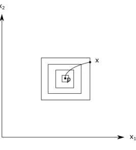
Figure 3.3: Ifn=2, any point x, pinR2+is on the boundary of some boxKa,b, and the trajectory throughx
moves through smaller and smaller nested boxes toward p.
(3.4) and (3.5) such thatKa,b ⊂ Bδ/2(p). Sincep∈ω(x), there is somet0 >0 such that x·t0 ∈Ka,b, since Ka,bcontains a neighborhood of p. ButKa,bis forward invariant, so this means thatx·t∈Ka,b⊂ Bδ/2(p) for
allt≥t0. Hence,{x·t}t≥t0 stays bounded away fromq, which means thatq<ω(x). This is a contradiction.
Thus, we conclude thatω(x)={p}for everyx∈Rn+.
See Figure 3.3 for an illustration of how a trajectory starting at somexmoves into smaller and smaller nested boxes towardpwhenn=2.
3.2 Nonconstant Albedo
In the last section, we showed that there is one globally attracting equilibrium if albedo is constant. However, it is more realistic to think of albedo as a function of temperature, so here we will look at what happens to solutions of (3.1) when we allow albedo to depend on the temperature of the ground. Forg(x1),
we follow the example of [31] and use
g(x1)=a˜ + b˜−a˜
2 1+tanh
x1−x∗ x0
!!
, (3.6)
where 0≤a˜ <b˜,x∗∈R, andx0>0. As we will see, different choices of these parameter values will lead to
100 200 300 400 200 400 600 800 1000
100 200 300 400
200 400 600 800 1000
100 200 300 400
200 400 600 800 1000
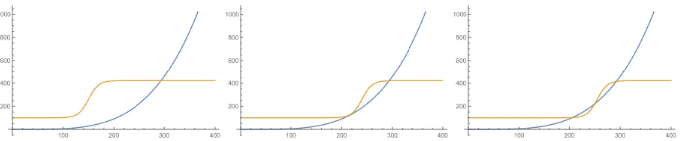
Figure 3.4: The graphs ofy=g(x1) (yellow) andy= σnx41(blue) may intersect at one, two, or three positive x1-values.
As stated in the introduction of this chapter, the equilibria of (3.1) are points of the form
p=
c, 4
r
n−1
n c,
4
r
n−2
n c, . . . ,
4 r 1 nc
, (3.7)
wherec∈h0. Depending on the number of layersnand the parameter values forg, we can get one, two, or
three equilibria, as shown in Figure 3.4.
The case of two equilibria can be viewed as a bifurcation as the system passes from having one equilibrium to three, or vice versa. For our analysis, we will focus on the behavior of the system when there is one equilibrium or when there are three. Specifically, when there is one equilibrium, we would like to know if it is globally attracting, as in the case with constant albedo. And when there are three equilibria, what is the stability of each fixed point? We get an idea of what the behavior of the system might be whenn=1 (this is known as thebare rock model, where there is no atmosphere):
˙
x1=g(x1)−σx41.
If there are three equilibria here, it is clear from looking at the sign ofg0(x1)−4σx13that the two outer fixed
points are attracting, while the fixed point between them is not. Does this still hold when there are an arbitrary number of layers of atmosphere?
To answer these questions, we try to obtain similar results to those in Section 3.1. To start, we look at the derivative matrix evaluated at a fixed point p=
c, 4
q
n−1 n c,
4
q
n−2 n c, . . . ,
4
q
1 nc
, which has the form
D f(p)=4σ c
4
n
!3/4
where
Pn(c)=
g0(c)n3/4 4σc3 −n3
/4 (n−1)3/4 0 · · · 0 0
n3/4 −2(n−1)3/4 (n−2)3/4 · · · 0 0
0 (n−1)3/4 −2(n−2)3/4 · · · 0 0
0 0 (n−2)3/4 · · · 0 0
... ... ... ... ... ...
0 0 0 · · · −2(2)3/4 1
0 0 0 · · · 23/4 −2
(3.8)
Similar arguments to those in Section 3.1 show thatD f(p) is diagonalizable and has all real eigenvalues. Furthermore,D f(p) is invertible, provided we make the following assumption:
(A1) Ifc∈h0andhchanges signs atc, thenh0(c),0.
This is a reasonable assumption if there are one or three fixed points; see Figure 3.4.
We can also find forward invariant boxes around some of the fixed points, similar to those in Section 2. Proposition 3.2.1. Suppose a=(a1, . . . ,an)∈Rn+satisfies
a1 ∈h+
a41− g(a1)
σ <a42 < n−1
n a41
2a4i−1−a4i−2 <a4i < nn−−ii++12a4i−1, for all i∈ {3, . . . ,n}
(3.9)
and b=(b1, . . . ,bn)∈Rn+satisfies
<b1 ∈h−
n−1
n b41 <b42 <b41− g(b1)
σ
n−i+1 n−i+2b
4 i−1 <b
4 i <2b
4 i−1−b
4
i−2, for all i∈ {3, . . . ,n}


![Figure 3.6: The transfer of radiation between the Earth and atmosphere in the leaky greenhouse model when n = 3 and ε ∈ (0, 1].](https://thumb-us.123doks.com/thumbv2/123dok_us/8228369.2181215/48.918.262.663.475.627/figure-transfer-radiation-earth-atmosphere-leaky-greenhouse-model.webp)

