Brandon_unc_0153D_15557.pdf

NOVEL INTEGRATION IN TIME METHODS VIA DEFERRED

CORRECTION FORMULATIONS AND SPACE-TIME

PARALLELIZATION

Namdi Brandon

A dissertation submitted to the faculty at the University of North Carolina at Chapel Hill in partial

fulfillment of the requirements for the degree of Doctor of Philosophy in the Department of

Mathematics in the College of Arts and Sciences.

Chapel Hill

2015

ABSTRACT

Namdi Brandon: Novel Integration in Time Methods via Deferred

Correction Formulations and Space-Time Parallelization

(Under the direction of Jingfang Huang)

ACKNOWLEDGEMENTS

First of all, I would like to thank my adviser, Jingfang Huang, for his support and wisdom over

these years. I also would like to thank my committee members David Adalsteinsson, Gregory Forest,

Laura Miller, and Jan Prins. I would also like to thank Michael Minion and Matthew Emmett for

their help and patience in helping me with the beginning of my research. I would like to thank the

NSF for providing me financial support during my studies.

I would like to sincerely thank all of my friends that I made during this program. Without their

support at work or at play, I could not have made it.

TABLE OF CONTENTS

LIST OF FIGURES . . . .

x

LIST OF TABLES . . . .

xii

INTRODUCTION . . . .

1

0.1

The State of Computing . . . .

1

0.2

Overview of Numerical Methods

. . . .

1

0.3

Stiff Ordinary Differential Equations . . . .

2

0.4

Overview of Dissertation . . . .

3

CHAPTER 1: FAST MULTIPOLE METHOD . . . .

5

1.1

Poisson Equation . . . .

5

1.1.1

Green’s Function . . . .

6

1.1.2

Coulomb Potential . . . .

7

1.2

Multipole and Local Expansions

. . . .

8

1.2.1

Multipole Expansion . . . .

9

1.2.2

Local Expansion . . . .

11

1.3

The

O

(

N

) Algorithm . . . .

12

1.3.1

Translation of the Multipole Expansion . . . .

13

1.3.2

Conversion to a Local Expansion . . . .

14

1.3.3

Translation of the Local Expansion . . . .

14

1.3.4

The Algorithm Outline

. . . .

15

1.4

Multirate FMM . . . .

15

CHAPTER 2: DEFERRED CORRECTION METHODS . . . .

19

2.1

Collocation Formulations and Properties . . . .

20

2.1.1

Gauss Collocation Method . . . .

21

2.1.2

Different Collocation Formulations . . . .

23

2.2

Deferred Correction Methods and Properties

. . . .

26

2.2.1

Backward Euler Preconditioned SDC for yp-Gauss Collocation Formulation .

26

2.2.2

Backward Euler Preconditioned SDC for integral-Gauss Collocation Formulation 28

2.2.3

Understanding Deferred Correction Iterations . . . .

30

2.2.4

Properties of Deferred Correction Iterations . . . .

34

2.2.5

Different Deferred Correction Methods . . . .

42

2.2.6

Integral Formulation, yp-formulation, and Convergence

. . . .

51

2.3

Algorithm Design Guidelines and Numerical Experiments . . . .

52

2.3.1

Optimal Collocation Formulation . . . .

53

2.3.2

Techniques for Convergence Procedure . . . .

54

2.4

Mapping Between Different Node Points . . . .

59

CHAPTER 3: A NEW JACOBIAN-FREE NEWTON-KRYLOV METHOD

. .

61

3.1

Krylov Methods

. . . .

61

3.1.1

GMRES . . . .

61

3.1.2

Inexact GMRES . . . .

62

3.2

General JFNK Methods . . . .

65

3.3

Modified JFNK Method . . . .

67

3.3.1

Deferred Correction Methods . . . .

67

3.3.2

Properties . . . .

68

3.3.3

The Krylov Subspace

. . . .

69

3.3.4

Newton’s Method . . . .

69

3.4

Algorithm Design . . . .

73

3.5

Numerical Experiments

. . . .

75

3.5.1

Cosine Problem . . . .

76

3.5.3

Nonlinear Multimode Problem . . . .

78

3.5.4

Van der Pol Oscillator . . . .

79

CHAPTER 4: PARALLEL FULL APPROXIMATION SCHEME IN SPACE AND

TIME . . . .

82

4.1

Temporal Methods . . . .

82

4.1.1

Spectral Deferred Corrections . . . .

82

4.1.2

Parareal . . . .

83

4.1.3

Full Approximation Scheme . . . .

86

4.1.4

Parallel Full Approximation Scheme in Space and Time . . . .

87

4.2

Spatial Methods

. . . .

89

4.2.1

Grid Systems . . . .

90

4.2.2

Gridless Systems . . . .

90

CHAPTER 5: A PFASSTER APPLICATION: GEOCHEMICAL PROBLEM . .

91

5.1

Formulation . . . .

91

5.2

PFASST Simulation . . . .

94

5.2.1

Results

. . . .

95

CHAPTER 6: A PFASSTER APPLICATION: N-BODY SOLVER

. . . .

98

6.1

PFASST Simulation . . . .

98

6.1.1

Temporal Coarsening

. . . .

99

6.1.2

Multirate Fast Multipole Method . . . .

99

6.1.3

Step size . . . 100

6.1.4

Spatial Coarsening . . . 101

6.2

Numerical Results

. . . 102

6.2.1

Numerical Setup . . . 102

6.2.2

Results

. . . 103

6.2.3

The Residual Equation

. . . 107

6.2.4

Gravitational Forces . . . 110

6.3

Speedup . . . 112

CHAPTER 7: FUTURE WORK . . . 115

APPENDIX A: PROOFS OF THEOREMS . . . 117

A.1 Proof of Theorem 2.2.3. . . 117

A.2 Proof of Theorem 2.2.4. . . 117

LIST OF FIGURES

1.1

Results of the multirate test . . . .

17

2.1

Accuracy in

x1

for different step sizes using (a) traditional BDF methods, orders 2,

3, 4 (from [1]) and (b) Gauss collocation methods using 3, 4, 5 Gaussian nodes. . . .

23

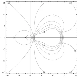
2.2

Contour of

ρ

(

C

(

λ

∆

t

)) for

p

= 4 for

SDC,

λ

∆

t

=

x

+

iy

. . . .

35

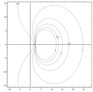
2.3

Contour of

ρ

(

C

(

λ

∆

t

)) for

p

= 10 for

SDC,

λ

∆

t

=

x

+

iy

.

. . . .

35

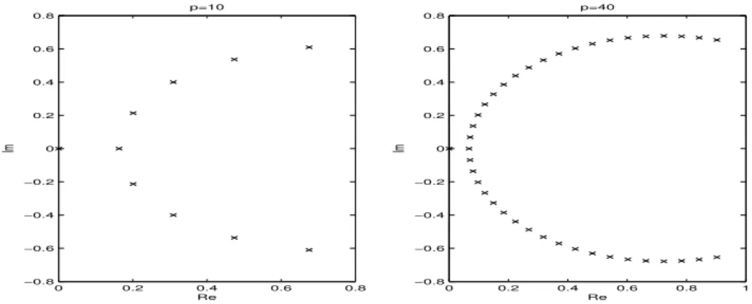
2.4

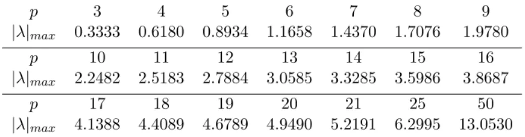
Distributions of correction matrix eigenvalues for

p

= 10 and

p

= 40, stiff case,

SDC.

37

2.5

Modulus of the (a) largest and (b) second largest eigenvalues for different numbers of

nodes,

SDC vs. Picard for the Gauss collocation formulation

. . . .

37

2.6

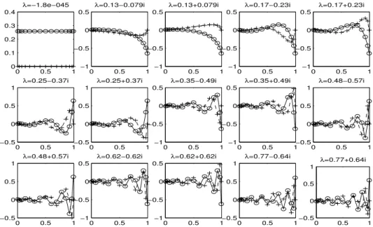
Eigenvalue distributions of SDC and Picard iterations for (a) 10 nodes and (b) 20

nodes

. . . .

38

2.7

S

−

S

˜

: Real (

o

) and imaginary (+) components of each eigenvector at the collocation

points, non-stiff case,

p

= 15,

SDC.

. . . .

39

2.8

S

: Real (

o

) and imaginary (+) components of each eigenvector at the collocation

points, non-stiff case,

p

= 15,

Picard iteration

. . . .

39

2.9

How errors decay after each SDC or Picard iteration.

. . . .

40

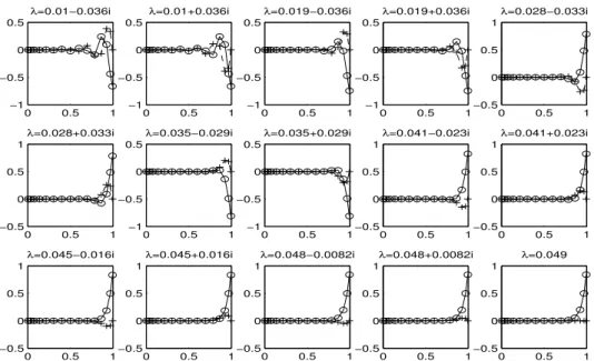
2.10 Real (

o

) and imaginary (+) components of each eigenvector at the collocation points,

stiff case,

p

= 15,

backward Euler preconditioned Gauss collocation formulation.

. . .

41

2.11 Contour of

ρ

(

C

) for

p

= 4 for

SDC-Radau,

λ

∆

t

=

x

+

iy

.

. . . .

43

2.12 Contour of

ρ

(

C

) for

p

= 10 for

SDC-Radau,

λ

∆

t

=

x

+

iy

.

. . . .

44

2.13 Contour of

ρ

(

C

) for

p

= 4, SDC-Lobatto methods,

λ

∆

t

=

x

+

iy

.

. . . .

45

2.14 Contour of

ρ

(

C

) for

p

= 10, SDC-Lobatto methods,

λ

∆

t

=

x

+

iy

.

. . . .

46

2.15 Contour of

ρ

(

C

) for

p

= 4 for

InDC-yp,

λ

∆

t

=

x

+

iy

. . . .

47

2.16 Contour of

ρ

(

C

) for

p

= 5 for

InDC-yp,

λ

∆

t

=

x

+

iy

. . . .

48

2.17 Contour of

ρ

(

C

) for

p

= 10 for

InDC-yp,

λ

∆

t

=

x

+

iy

.

. . . .

49

2.18 Spectral Radius

ρ

(

S

−

S

˜

) for different numbers of nodes,

Lobatto and

SDC-Lobatto-T.

. . . .

50

2.19 Convergence rate for backward Euler preconditioned Gauss (a) and uniform (b)

collocation formulations for different stiffness parameters

λ

. . . .

59

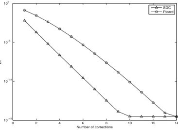
the relative error of the final iteration vs. the collocation formulation . . . .

78

3.3

Nonlinear multimode problem. (a): the magnitude of the deferred correction

.

(b): the relative error of the final iteration vs. exact solution

. . . .

79

3.4

Van der Pol oscillator. (a): the magnitude of the deferred correction

. (b): the

relative error of the final iteration vs. the collocation formulation . . . .

80

5.1

Relative error of

L

(c) per iteration over time using SDC . . . .

95

5.2

Relative error per iterations for each

c

at

t

. . . .

96

5.3

Relative error of

L

(c) per iteration over time, PFASST . . . .

96

5.4

Relative error per iterations for each

c

at

t

. . . .

97

6.1

Multirate test for electrostatic case . . . 101

6.2

Absolute error of velocity per iteration compared to the reference solution.

Coarse-level FMM precision is

_{= 0}

_.

₅

_×

₁₀

_{. . . 104}

6.3

Absolute error of velocity per iteration compared to the reference solution.

Coarse-level FMM precision is

= 0

.

5

×

10

. . . 105

6.4

Absolute error of velocity per iteration compared to the reference solution.

Coarse-level FMM precision is

= 0

.

5

×

10

. . . 105

6.5

Relative error of velocity per iteration to

V

with coarse-level FMM precision

_{= 0}

_.

₅

_×

₁₀

_{. . . 105}

6.6

Relative error of velocity per iteration to

V

with coarse-level FMM precision

= 0

.

5

×

10

. . . 106

6.7

Relative error of velocity per iteration to

V

with coarse-level FMM precision

= 0

.

5

×

10

. . . 106

6.8

Multirate test for gravitational case . . . 110

6.9

Absolute error of velocity per iteration compared to the reference solution.

Coarse-level FMM precision is

= 0

.

5

×

10

. . . 111

LIST OF TABLES

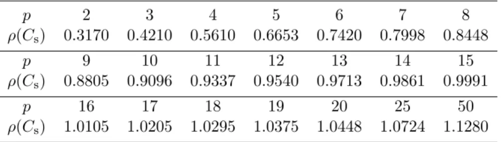
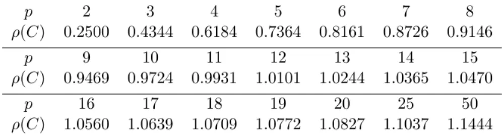
2.1

ρ

(

Cs

) for different numbers of Gaussian nodes, stiff case,

SDC.

. . . .

36

2.2

ρ

(

C

) for different numbers of nodes,

SDC-Radau.

. . . .

42

2.3

ρ

(

C

) for different numbers of nodes,

SDC-Lobatto methods.

. . . .

45

2.4

ρ

(

C

) of SDC-Lobatto-T, strongly stiff limit case. . . .

48

2.5

Errors from Gauss and uniform collocation formulations for different numbers of nodes.

53

2.6

Errors and Orders of the backward Euler and trapezoidal rule preconditioned deferred

correction iterations for different collocation formulations, non-stiff case. . . .

55

2.7

Errors and orders of the backward Euler preconditioned deferred correction iterations

for different collocation formulations, stiff case. . . .

58

3.1

The number of

H

(˜

y) needed to converge.

. . . .

80

3.2

The relative correction log

of the converged solution. . . .

80

5.1

Timing results for SDC and PFASST . . . .

97

6.1

Runtime for various FMM precisions . . . 101

6.2

Serial SDC, 6 iterations . . . 112

6.3

PFASST, 7 iterations . . . 112

INTRODUCTION

0.1

The State of Computing

In 1965, the co-founder of Intel, Gordon Moore, predicted that the transistor density of

semi-conductor chips, hence the CPU speed, would double roughly every 1

.

5 years. This prediction has

become known as

Moore’s law; and from 1965 to about 2002, Moore’s law was upheld [45]. However,

as the transistor density increased, the power density of the chip increased causing greater levels of

heat on the chip. Technology has reached a point where the speed of processors cannot increase

much further due to this limitation. Hence in 2005, a paradigm shift occurred in processor design

in hopes of further increasing computational performance. Instead of creating ever-faster CPUs

running computations in

serial, additional performance can be gained by having

multiple

processors

work together, or in

parallel

[45].

The ability of having ever increasing computational power and efficient numerical methods

that can take advantage of this power has lead to great advances in science. As computational

power increases, so does the number of problems previously considered impractical to solve become

feasible. Therefore, creating methods to solve these problems is also an increasingly important

field of research. The following are a few examples of areas of open problems that require much

computational power: climate modeling, data analysis, and molecular dynamics (protein folding

and drug discovery).

0.2

Overview of Numerical Methods

ODE IVPs such as DASPK, a backward differentiation formula (BDF) based solver [10, 41], and

Runge-Kutta method based Radau5 solvers [24]. Numerical solvers have been successfully applied in

research and have advanced our knowledge in science and engineering. However, there still presides

attributes that limit the effectiveness of existing numerical algorithms. For example, to understand

the evolution of charged particles in systems containing thousands of particles, current molecular

dynamics simulation tools usually require millions of time steps to accurately capture the motion of

particles using existing low order time stepping schemes (e.g., the Verlet integration scheme). Even

with the acceleration of the fast

N

-body solvers [22, 43] for each time step, simulations may require

weeks or longer to get physically relevant results.

In recent years, several schemes were introduced to address the challenges in designing accurate

and efficient algorithms for large-scale long-time simulations.

Examples include the parareal

algorithm for parallelization in time [18, 42]; the high order temporal discretization using an

orthogonal basis and pseudo-spectral formulations for each time step, to allow larger step sizes

[6, 43, 38]; the spectral deferred correction (SDC), integral deferred correction (InDC), iterated

defect correction (IDeC), and Krylov deferred correction (KDC) methods for their efficient solutions

[3, 14, 16, 30]; and the parallel full approximation scheme in space and time (PFASST), which

utilizes parallel computing while combining several preconditioners [17]. The aim of the research

presented in this dissertation is to understand the properties of these existing methods and create

new methods that take advantage and possibly enhance their favorable traits such as high accuracy,

high efficiency, and parallelism.

0.3

Stiff Ordinary Differential Equations

slightly at any time, the resulting curve through the perturbed data has rapid variation. Typically

this takes the form of a short lived “transient” response that moves the later solution back toward a

smooth solution.” To understand stiffness, consider the following ODE

y

(

t

) =

λ

(

y

(

t

)

−

cos(

t

) )

−

sin(

t

)

.

(1)

where

<(

λ

)

<

0. A solution to this equation is

y

(

t

) = cos(

t

) with the initial condition

y

(0) = 1.

Notice that this smooth solution is the solution for any value of

λ

. If the initial data is

y

(

t0

) =

η

,

which does not lie on the curve cos(

t

), then the solution through this point is

y

(

t

) =

e

(

η

−

cos(

t

) ) + cos(

t

)

(2)

One can verify that this is true through differentiation. Since

<(

λ

)

<

0, the function approaches

cos(

t

) exponentially with decay rate

λ

. When one perturbs the solution at some point, the perturbed

solution approaches the slow changing particular solution cos(

t

).

The reason why stiff systems pose hardships on numerical methods for time dependent differential

equations is because stiff systems require algorithms to take a much smaller time step in order for

an algorithm to be stable. Although the true solution is smooth and it seems that a large time step

would suffice, the numerical method must handle the rapidly changing signal by taking smaller time

steps in order to attain accuracy. This property of stiff systems increases the runtime of simulations

and limits their effectiveness. This documents presents research aimed at overcoming the limitations

given by stiff systems.

0.4

Overview of Dissertation

CHAPTER 1

Fast Multipole Method

In this chapter, we will present a brief overview of the spatial method used for modeling the

evolution of charged particles in a vacuum. In this dissertation, we are using the electrostatics

assumption, which states that the charge density, denoted by

ρ

, is stationary or the charge density

does not change quickly in time. That is,

= 0 or

1.

With that being said, the evolution of

N

charged particles in space is given by Newton’s 2

law. For the

i

particle, the equation of motion is

d

x

(

t

)

dt

=

q

m

E(x

(

t

))

(1.1)

where

x

is the position,

E

is the electric field,

q

is the charge, and

m

is the mass of the

i

particle.

Therefore, solving this system consists of two steps. (1) Finding an expression for the electric field.

We will designate this as the

spatial calculation. (2) Once the electric field is calculated, integrating

in time to find the new position of the particle. We will designate this as the

temporal calculation.

What follows is an explanation on how to solve for the electric field.

1.1

Poisson Equation

The electrostatic field in a vacuum is described by two of the Maxwell’s equations

∇ ·

E

=

ρ

(1.2)

where

ρ

(

x

) is the charge density within a volume and the constant

is the permeability of free

space [32]. Eq. (1.3) is equivalent to expressing

E

as the gradient of a scalar function Φ(x) such that

E

=

−∇Φ

.

(1.4)

Φ is called the electrostatic potential. Combining Eq. (1.4) and Eq. (1.2), we can write the vector

equation for

E

in terms of a scalar equation for Φ

∇

_{Φ =}

₋

ρ

0

.

(1.5)

The above equation is called the

Poisson equation. In regions of space lacking a charge density,

Poisson’s equation becomes the

Laplace equation

∇

Φ = 0

.

(1.6)

Hence, solving the spatial calculation for

E

in Eq. (1.1) is equivalent to solving the Poisson equation.

1.1.1

Green’s Function

The solution to the Poisson equation Eq. (1.5) within a volume

V

bounded by a surface

S

can

be found by using a construct called a

Green’s function,

G

(x

,

x

). The Green’s function for Eq. (1.5)

has the property that it is a fundamental solution to the following equation

∇

G

(x

,

x

) =

−4

πδ

(x

−

x

)

.

(1.7)

Assuming we have found the solution

G

(x

,

x

) to the above equation, the general solution Φ to the

Poisson equation is

Φ(x) =

1

4

π0

Z

V

ρ

(x

)

G

(x

,

x

) d

x

+

1

4

π

I

S

G

(x

,

x

)

∂

Φ

∂n

−

Φ(x

)

∂G

(x

,

x

₎

∂n

where

n

is the normal direction pointing out of the surface and d

a

is the area element [32].

Fortunately, there is an explicit formulation of the Green’s function for electrostatic problems; it is

G

(x

,

x

) =

1

|x

−

x

|

.

(1.9)

1.1.2

Coulomb Potential

Recall that we are interested in finding the potential in free space. The relevant boundary

conditions are the Dirichlet conditions. Therefore, we must have that Φ(x)

→

0 as

x

→ ∞. In

addition, we also have the Green’s function satisfy Dirichlet conditions

G

|

= 0 in Eq. (1.7).

Applying the Dirichlet boundary conditions and the appropriate Green’s function, Eq. (1.8) becomes

Φ(x) =

1

4

π

Z

V

ρ

(x

)

|x

−

x

_|

d

3

_x

_.

_(1.10)

The above equation is called the

Coulomb potential, and it gives the electrostatic potential subject

to the Dirichlet condition in free space for a general charge distribution

ρ

(x).

By modeling a charged particle as a point charge, we can write the charge density distribution

of

N

charged particles as

ρ

(x) =

N

X

i=1

q

δ

(x

−

x

)

where

q

is the charge of a particle located at

x

[32]. Using the above charge distribution in

Eq. (1.10) leads to the Coulomb potential for

N

charged particles

Φ(x) =

1

4

π

N

X

j=1

q

|x

−

x

|

.

(1.11)

We now have all of the components needed to write an explicit formulation for the equations of

motion for a system of

N

charges. Using

E

=

−∇Φ and Eq. (1.11), we can express Eq. (1.1) as

d

x

(

t

)

dt

=

−

q

m

where

Φ

(x

) =

1

4

π

N

X

j6=i

q

|x

−

x

|

.

(1.13)

Occasionally in this dissertation, we will make reference to the forces instead of the potential in

Eq. (1.12). The force

F

is related to the electric field, and hence, the electrostatic potential by

F

=

q

E

=

−

q

∇Φ. Using the identity

∇

1

|x

−

x

_|

=

−

x

−

x

|x

−

x

_|

,

the force of the

i

particle is given by

F

(x

) =

−

q

∇Φ

(x

) =

q

X

j6=i

q

x

−

x

|x

−

x

|

.

(1.14)

1.2

Multipole and Local Expansions

The cost of directly calculating the potentials Φ

(x

) in Eq. (1.12) for all

N

particles is

O

(

N

).

When

N

is large, this cost is too high. In actual applications, we avoid the direct

O

(

N

) calculation

by using approximations. The approximation technique that this dissertation uses is the fast

multipole method (FMM), which approximates Eq. (1.13) over all particles with cost

O

(

N

) [22, 43].

The FMM takes advantage of the fact that the potential Φ(x) can be written as a a sum of

potentials from two different spatial domains. This property comes from the Green’s function

G

(x

,

x

) =

1

|x

−

x

_|

which has spatial multirate properties. We define the following spatial domains Ω

and Ω

,

which we will denote as the near-field and the far-field, respectively. For a given location

x, a charge

found at

x

has

x

∈

Ω

with respect to

x

if

|x

−

x

|

< R

. And we consider

x

∈

Ω

with

respect to

x

if

|x

−

x

| ≥

R

where

R

is the characteristic distance that determines the near-field

and far-field. In Ω

, the Green’s function is smooth; and in Ω

, the Green’s function is more

1.2.1

Multipole Expansion

Assuming that

|x|

>

|x

|, it is convenient to express the Green’s function in terms of the series

1

|x

−

x

_|

=

1

|x|

∞

X

n=0

P

(cos

θ

)

_|x

_|

|x|

(1.15)

where

P

are the Legendre polynomials and

θ

is the angle between

x

and

x

. Normally,

x

corresponds

to the position of a source charge, so our assumption implies that

x

is far from a charge found at

x

.

This expansion is especially useful in describing far field interactions, since the expansion converges

quickly when

<

1.

The Legendre polynomial

P

(

u

) is the solution to the following recursion formulation

(2

n

+ 1)

uP

(

u

) = (

n

+ 1)

P

(

u

) +

nP

(

u

)

with

P

(

u

) = 1. We can further expand the Legendre polynomials in terms of spherical harmonic

functions

P

(cos

θ

) =

X

m=−n

Y

(x

)

Y

(x)

(1.16)

to obtain a new formulation of the Green’s function in Eq. (1.15)

1

|x

−

x

_|

=

∞

X

n=0

m=n

X

m=−n

|x

|

Y

(x

)

Y

m n

(x)

|x|

.

(1.17)

If we express

x

in spherical coordinates (

r, θ, φ

), the spherical harmonic function

Y

(x) is

defined as

Y

(

θ, φ

) =

s

(2

n

+ 1)

4

π

(

n

−

m

)!

(

n

+

m

)!

·

P

|m|

n

(cos

θ

)

e

(1.18)

where

P

n

are the

associated Legendre polynomials

[32, 52, 31]. The associated Legendre polynomials

P

are found by the following formulations















P

(

u

)

= (1

−

u

)

m

∂um

P

(

u

)

P

n

(

u

)

= (−1)

(n−m)!

(n+m)!

P

(

u

)

.

expressed in spherical coordinates due to

N

charged particles at positions

x

= (

r

, θ

, φ

) in

Eq. (1.11) as

Φ(x) =

1

4

π0

X

q

X

m=n

X

m=−n

|x

|

_Y

(x

)

Y

(x)

|x|

(1.19)

=

1

4

π0

∞

X

n=0

m=n

X

m=−n N

X

i=1

q

|x

|

Y

(x

)

Y

(x)

|x|

.

The terms

are called “multipoles,” and their coefficients

M

=

N

X

i=1

q

|x

|

Y

(x

)

(1.20)

are called

moments

of the expansion. Using the the moments

M

n

, we can rewrite the potential as

Φ(x) =

1

4

π

∞

X

n=0

m=n

X

m=−n

M

Y

m n

(x)

|x|

.

(1.21)

The above formulation for the potential is called the

multipole expansion. Notice that if

|x|

is

large when compared to the charge locations

|x

|, the multipole expansion will converge quickly.

Due to this property, we can approximate the infinite sum by truncating the series with

p

terms

Φ

(x) =

1

4

π

p−1

X

n=0

m=n

X

m=−n

M

Y

m n

(x)

|x|

;

(1.22)

and the residual error of the truncated series is bounded by

|Φ(x)

−

Φ

(x)|

=

Q

|x| − |x

|

|x

|

|x|

(1.23)

where

Q

=

N

P

i=1

|

q

|

,

|x

|

and

|x

|

are the minimum and maximum magnitude of

|x

|, respectively.

Note that the amount of calculations needed to calculate Φ

(x) is

O

(

p

).

If we partition space into regions or “boxes” Ω

of radius

R

that contain various charges found

at

x

∈

Ω

, the multipole expansion approximation Φ

(x) is useful in expressing the potential Φ

due to the particles within Ω

when the point of interest

x

is far from region Ω

. By far, we mean

expansion” with the respect to region Ω

.

1.2.2

Local Expansion

The multipole expansion approximation assumes that the source particles are in the near field

with respect to an origin,

x

∈

Ω

; and the point of interest is in the far field from the origin

x

∈

Ω

. However, when the case is reversed,

x

Ω

and

x

Ω

with respect to an origin, we

will need a new formulation for the potential Φ. We can use Eq. (1.19) and exchange the vectors

x

and

x

to obtain

Φ(x) =

1

4

π

N

X

q

X

m=n

X

m=−n

|x|

Y

(x)

Y

(x

)

|x

|

(1.24)

=

1

4

π

∞

X

n=0

m=n

X

m=−n N

X

i=1

q

Y

(x

)

|x

|

|x|

n

_Y

(x)

.

The above series converges when

<

1. We can express the moments of this expansion

L

as

L

=

N

X

i=1

q

Y

(x

)

|x

|

and rewrite the potential as

Φ(x) =

1

4

π0

∞

X

n=0

m=n

X

m=−n

L

|x|

_Y

n

(x)

.

(1.25)

The above formulation for the potential is called the

local expansion. Notice that if

|x|

is small

when compared to the charge locations

|x

|, the local expansion will converge quickly. Due to this

property, we can approximate the infinite sum by truncating the series with

p

terms

Φ

(x) =

1

4

π

p−1

X

n=0

m=n

X

m=−n

L

|x|

Y

(x)

.

(1.26)

1.3

The

O

(

N

)

Algorithm

The FMM works by using a tree structure to partition space into boxes that contain certain

numbers of particles [22]. For each box

m

, we define the following spatial domains Ω

and Ω

,

which we will denote as the near-field and the far-field, respectively. For a given location

x, a charge

found at

x

has

x

∈

Ω

with respect to

x

if

|x

−

x

|

< R

. And we consider

x

∈

Ω

with

respect to

x

if

|x

−

x

| ≥

R

where

R

is the characteristic distance that determines the near-field

and far-field.

In short, the FMM approximates Eq. (1.11) by directly calculating potential due to particles in

the near-field and approximating the potential due to particles in the far-field. We can express the

FMM approximation Ψ(x) such that Ψ(x)

≈

Φ(x) as

Ψ(x) =

1

4

π





X

xiΩnear

q

|x

−

x

|

+

p−1

X

j=0

a

|x

−

x

|





.

(1.27)

We will call Eq. (1.27) the

fast multipole approximation. In the expansion,

x

is the position

of the box center on the finest level containing

x; and

a

are coefficients that depend on

∀x

∈

Ω

.

p

is the number of terms in the expansion, and it controls the accuracy of Ψ(

x

). The larger

p

is,

the more accurate the FMM becomes. The first summation in Ψ(x) is the direct calculation of

the potential due to the near-field charges. The second summation in Ψ(x) is the approximation

of the potential due to the far-field. We will give a brief explanation of the FMM; but for more

information on the FMM, the reader is encouraged to read [22, 31].

For an arbitrary distribution of particles, the FMM uses a hierarchical oct-tree so that each

particle is associated with a box at different levels. Each box

i

has a “parent box” on the next-coarse

level to which the

i

box is a subset. A box

i

is a “child box” of box

j

if

i

is on the

j

’s subsequent

fine level and

i

is a subset of

j

. A divide-and-conquer strategy is used to account the far-field

interactions of each box on each level by accumulating multipole expansions. Afterwards, the local

expansion of a parent box receives the far-field contributions and transmits it to its children [52].

The fast multipole method needs the following properties to approximate the

O

(

N

) calculation

in Eq. (1.13) in

O

(

N

) [31].

coarse-grid expansion.

2. The FMM needs a way to combine several multipole expansions into a single local expansion

about origin of a target box on the same level.

3. The FMM needs a way to translate a box’s local expansion to an origin within each of the

child boxes at the following fine level of the tree.

1.3.1

Translation of the Multipole Expansion

The following expansion allows us to combine several multipole expansions of one level into a

single expansion on a coarser level. If we have a multipole expansion about the origin, we can shift

the expansion and center it at a point

z

[31]. The original expansion about the origin

Φ(x) =

1

4

π

∞

X

n=0

m=n

X

m=−n

M

Y

m n

(x)

|x|

can be written as an expansion about

z

as

Φ(x) =

1

4

π0

∞

X

n=0

m=n

X

m=−n

˜

M

Y

m

n

(x

−

z)

|x

−

z|

where

˜

M

=

n

X

j=0

j

X

k=−j

M

i

|m|

i

_i

A

A

A

|z|

Y

(z)

and the constant

A

is defined by

A

=

(−1)

n

p

(

n

−

m

)!(

n

+

m

)!

.

The error bounds of the truncated expansion is

|Φ(x)

−

Φ

(x)| ≤

Q

|x

−

z| − |x

| − |z|

|x

|

+

|z|

|x

−

z|

1.3.2

Conversion to a Local Expansion

The following shows how to convert a multipole expansion to a local expansion on the same

level. We must assume that the new center at

−z

must be far enough away from the multipole

expansion assumed at the origin such that

|z|

>

(1 +

c

)|x|.

Φ(x) =

1

4

π

∞

X

n=0

n

X

m=−n

L

|z

−

x|

Y

(z

−

x)

where

L

=

X

j=0

j

X

k=−j

M

(−1)

i

i

_i

A

A

A

Y

(z)

|z|

and

A

j

is defined as before. The error bounds of a truncated expansion with

p

terms, Φ

is

|Φ(x)

−

Φ

(x)| ≤

Q

(

c

−

1)|x|

1

c

.

1.3.3

Translation of the Local Expansion

To shift a local expansion of a box on the parent level to a box center of the child box at

−z, we

start with the local expansion given by

Φ

(x) =

1

4

π0

p−1

X

n=0

m=n

X

m=−n

L

|x|

Y

(x)

.

We can express the truncated expansion

Φ

(x) =

1

4

π0

p−1

X

n=0

m=n

X

m=−n

˜

L

|x

−

z|

Y

(x

−

z)

where

˜

L

=

X

j=0

j

X

k=−j

L

(−1)

i

i

_i

A

A

A

Y

k−m

j−n

(−z)|z|

1.3.4

The Algorithm Outline

The FMM consists of the following steps [31]:

1. Form multipole expansions (moments) at the finest scale.

2. Merge (translate) expansions to form expansions on the next coarser level until the coarsest

scale is reached.

3. Starting at the coarsest level, for each target region, convert the multipole expansion into

local expansion at the center of each target box.

4. For each box, merge (translate) the local expansion to the center of each of a box’s children

until the finest level is reached.

5. Add the near-field potential contribution from the nearest neighbors to the approximated

far-field potentials to obtain Eq. (1.27).

1.4

Multirate FMM

The FMM is an extremely useful method that takes advantage of the spatial properties of

the Coulomb potential Φ(x(

t

)). However, we can take advantage of the temporal properties of

the Coulomb potential and fast multipole approximation Ψ(x(

t

)) to make a less computationally

expensive algorithm.

From Eq. (1.14), one can see that the magnitude of the forces is proportional to

where

r

=

|x

−

x

|. When

x

∈

Ω

with respect to

x

, we can expect that the near-field forces should

change rapidly in time due to the

force with

r

small. When

x

∈

Ω

with respect to

x

, we can

expect that the far-field forces should change slowly in time due to the

force with

r

large. Thus,

we can represent the forces in Eq. (1.1) as

d

x

dt

=

−

q

m

This can be rewritten as

d

x

dt

=

−

q

4

π0m

∇





X

xj∈Ωnear

q

|x

−

x

|

+

X

xj∈Ωf ar

q

|x

−

x

|





.

This formulation suggests that the forces have a dual behavior as they change in time, reminiscent

of a stiff system. The total force has two different time scales: a fast changing near-field and a slow

changing far-field. Since the FMM approximation Ψ, defined in Eq. (1.27), approximates the right

hand side of Eq. (1.28), we should expect Ψ to uphold this multirate behavior. More importantly,

it should be possible to take account of this multirate behavior in time integration schemes. We

will call the process of exploiting the temporal multirate behavior of the FMM as the

multirate

FMM

(MRFMM).

1.4.1

Numerical Evidence

To test our hypothesis of the inherent temporal multirate behavior of the FMM, we ran numerical

experiments to see how the far-field and near-field potentials change in time. To do this, we simulated

the the motion of particles while keeping track of Ψ

(x(

t

)) and Ψ

(x(

t

)) for each time step. Once

the simulation is over, for a given particle, we calculated the respective least-squares polynomial that

approximates Ψ

(x(

t

)) and Ψ

(x(

t

)) over time. Afterwards for each time step, we calculated

the

L

norm of the error between Ψ

(x(

t

)) and Ψ

(x(

t

)) and their respective least-squares

approximating polynomial over all particles.

For a fixed

L

error, the slower a potential varies in time (ie. a smoother potential), the lower

the degree of the least-squares polynomial is needed. Our intuition says that for a fixed error

between the numerical FMM solution and the least-squares polynomial, the least squares polynomial

corresponding to Ψ

(x) should have a lower degree than that of Ψ

(x). The results of the

experiment show this to be true. That is, for a fixed error, there is a difference in scale between

Ψ

(x) and Ψ

(x). One needs a least-squares polynomial of lower degree for Ψ

(x) than that

of Ψ

(x).

charge 1. They simply moved in space but did not have any effect on the potential due to neither

the source particles nor due the other target particles. The potential at the all locations were due

solely to the source particles. We also assumed that all particles have mass equal to 1.

The numerical experiment was done using 16,000 source particles and 16,000 target particles

randomly distributed in a unit cube. We used the FMM approximation Ψ(x) to approximate the

Coulomb potential Φ(x) such that the error tolerance in Ψ(x) was 0

.

5

×

10

. During the simulation,

the FMM tree was fixed as well. The simulation consisted of 200 time steps with size ∆

t

= 10

_so

that

t

= 0 and

t

= 2

×

10

. And the time-marching scheme that we used was the velocity

Verlet method, which is as follows

x(

t

)

=

x(

t

) +

v(

t

)∆

t

+

a(

t

)

2

∆

t

2

v(

t

)

=

v(

t

) +

∆

t

2

(a(

t

) +

a(

t

))

(1.29)

where ∆

t

=

t

−

t

;

x(

t

),

v(

t

), and

a(

t

) are the position, velocity, and acceleration, respectively

at time

t

=

t

[26]. The velocity Verlet method has many favorable properties. Namely, it is explicit,

O

(∆

t

), and symplectic [26]. For future reference, we will call running this experiment as the

multirate test.

Figure 1.1 shows the results of our experiment. We plot the

L

error over all target particles

between Ψ

(x) and Ψ

(x) and their respective least squares approximating polynomials for

various degrees. We represent the error logarithmically, showing the digits of precision in the error.

These results provide numerical evidence of the inherit temporal multirate behavior in the

FMM. We can see that for the same error, there is about a 3-degree separation in the least squares

polynomial between the smoother Ψ

(x) than Ψ

(x). That is for a fixed error, Ψ

(x) needs

a lower degree least-squares polynomial than that for Ψ

. This agrees with our intuition; the

CHAPTER 2

Deferred Correction Methods

It is desirable for algorithms to efficiently converge to solutions of large-scale long-time simulations

for ODEs with high accuracy. One way to obtain such high accuracy solutions is to create methods

that converge to high order temporal collocation formulations. Solvers that have been made to

directly calculate accurate collocation formulation solutions have shown to not be able to do so

efficiently. For example in [23, 25], the Gauss collocation formulations using only 2, 4, and 6 nodes

were implemented as geometric integrators for Hamiltonian systems. Unfortunately, numerical

results show that without the aid of deferred correction or other acceleration techniques, these

solvers may not be able to calculate a highly accurate solution as efficiently as other linear multistep

methods (see Fig. 5.1 in [23]). If an algorithm can obtain high accuracy at the cost of severely

reduced efficiency, the algorithm becomes impractical in application. Hence, it is of great importance

to create algorithms that obtain high accuracy while at the same time obtaining high efficiency.

This chapter is organized as follows. In Sec. 2.1, we study the

converged solution

by developing

the “collocation formulations database” for the numerical framework for solving ODE initial value

problems and by discussing the properties of each formulation. In Sec. 2.2, we start from the

backward Euler based spectral deferred correction methods and their convergence properties, and

then study different deferred correct methods to form the “deferred correction methods database” in

the

convergence procedure, an iterative procedure to reduce the errors in the provisional solution.

In Sec. 2.4, we discuss several algorithm design guidelines to integrate different components to

efficiently converge

to the solution of an

“optimal” discretization

in the numerical framework.

2.1

Collocation Formulations and Properties

For long time simulations, it is in general impractical to use one single step for the entire

interval from

t

= 0 to

t

(e.g., by using a spectral formulation for [0

, t

]). What is done

in practice is that the entire time interval is divided into a sequence of subintervals (time steps)

based on the properties of the solution and any step size constraints. In this section, we discuss

different collocation formulations for each time step. These collocation formulations differ in the

mathematical formulations, choices of collocation points, and numerical integration or differentiation

strategies. We leave the discussions of their accurate and efficient solutions to later sections.

(up to a prescribed precision), the numerical properties of the solution are then determined by the

properties of the collocation formulation, not the convergence procedure. Unlike existing analysis of

the deferred correction methods, this new viewpoint allows us to study the mathematical properties

of the framework (e.g., order and stability) by focusing on the converged solution of the collocation

formulation, and to consider the

convergence procedure

(describing how the iterations converge)

separately.

2.1.1

Gauss Collocation Method

We first present a variant of the well-studied Gauss collocation formulation (also referred to

as the Gauss Runge-Kutta (GRK) method) for ODE initial value problems

y

(

t

) =

f

(

t, y

(

t

)) with

given initial data

y

(0) [25, 28]. To march one step from

t

= 0 to

t

= ∆

t

, we define

Y

(

t

) =

y

(

t

) as

the new unknown function and recover

y

(

t

) using

y

(

t

) =

y

(0) +

R

0

Y

(

τ

)

dτ

. This will give what we

call the

“yp-formulation”

as

Y

(

t

) =

f

(

t, y

(0) +

Z

0

Y

(

τ

)

dτ

)

.

(2.1)

In the Gauss collocation formulation,

p

Gaussian quadrature nodes

t

= [

t

, t

,

· · ·

, t

]

are used

to discretize the yp-formulation in [0

,

∆

t

]. For the given function values

Y

= [

Y1, Y2,

· · ·

, Y

]

at the Gaussian nodes, we can construct the (

p

−

1)

degree Legendre polynomial expansion to

approximate

Y

(

t

) =

y

(

t

) where the coefficients are computed using the Gaussian quadrature rules.

We can integrate this interpolating polynomial analytically from 0 to

t

, where 1

≤

m

≤

p

, to

form a linear mapping that maps the function values

Y

to the integral of

Y

(

t

) at the node points.

Taking out the scalar factor ∆

t

in this mapping, the integral

R

0

Y

(

τ

)

dτ

can be approximated by

∆

tS

Y, where

S

is called the

“spectral integration matrix”

[21] which can be precomputed. The

discretized Gauss collocation formulation using

p

node points in the time interval [0

,

∆

t

] is given by

Y

=

F(t

,

y

+ ∆

tS

Y)

.

(2.2)

Theorem 2.1.1.

For ODE initial value problems, the Gauss collocation formulation in Eq. (2.2)

with

p

nodes is of order

2

p

(super convergence),

A

-stable,

B

-stable, symplectic (structure preserving),

and symmetric (time reversible). In addition, the error decays exponentially when

p

increases.

Interested readers are referred to [5, 27] for the proof of the theorem. These nice properties

allow the use of very large time step sizes when solving ordinary differential equation initial value

problems.

Comment:

The yp-formulation can be easily generalized to differential algebraic equations

(DAEs) of the form

F

(

t, y, y

) = 0, and the discretized system becomes

F(t

,

y

+ ∆

tS

Y

,

Y) =

0

.

Similar to the ODE case, the pseudo-spectral type collocation formulation allows much larger time

step sizes in the numerical simulation. In Fig. 2.1, we compare the Gauss collocation formulation

with traditional BDF methods for the DAE system from [1]













x

x

0













=













10

−

0

10(2

−

t

)

9

2−t

−1

9

t

+ 2

t

₋

₄

₀

























x1

x2

z













+













3−t

2−t

e

2

e

e

₍₂

₋

_t

₋

_t

₎













(2.3)

whose analytical solution is given by (

x

, x

, z

) =

e

, e

,

−

e

/

(2

−

t

)

10−4 10−3 10−2 10−1 10−12

10−10 10−8 10−6 10−4 10−2 100

Time Step ∆ t

Max Error

Errors in x 1(t)

Order 2

Order 3 Order 4

(a)

10−0. 9 10−0.8 10−0. 7

10−15 10−10 10−5

Errors in x ₁ (t)

Time step ∆ t

Max Error

p=3 p=4 p=5

(b)

Figure 2.1: Accuracy in

x

for different step sizes using (a) traditional BDF methods, orders 2, 3, 4

(from [1]) and (b) Gauss collocation methods using 3, 4, 5 Gaussian nodes.

2.1.2

Different Collocation Formulations

In the Gauss collocation formulation discussed in the previous section, the Legendre polynomial

based Gaussian quadrature nodes are used and the spectral integration matrix is constructed

accordingly for the yp-formulation. Other types of formulations, quadrature nodes, and numerical

differentiation or integration techniques have also been studied in the literature. In this subsection,

we present different collocation formulations to form our “collocation formulation database” for

ODE initial value problems.

For the ODE initial value problem

y

=

f

(

t, y

), most existing collocation formulations use

y

as

the unknown and solve the differential equation directly. In the “differential quadrature method” [13]

and other traditional pseudo-spectral collocation formulations, the “spectral differentiation matrix”

is constructed by differentiating the interpolating polynomial of

y

at the collocation points and

evaluating the derivative polynomial to form the spectral differentiation matrix

D

mapping

y

at the

collocation points to

y

. We refer to this class of formulations as the

“differential formulation,”

and the discretized ODE system can be represented as

D

y

=

f

(t

,

y). An alternative formulation is

to use the equivalent Picard integral equation formulation

y

(

t

) =

y0

+

R

f

(

τ, y

(

τ

))

dτ

and discretize

the ODE system as in

where

y

are the unknowns at the collocation points, and

S

is the (scaled) spectral integration

matrix. We refer to this formulation as the

“integral formulation.”

It is important to note that

when the spectral integration matrix is used, this integral formulation also converges to the Gauss

collocation formulation. When this formulation is coupled with uniform collocation points, the

resulting deferred correction methods are called the integral deferred correction methods (InDC)

[14]. In the previous subsection, we also presented the

“yp-formulation”

using

y

as the unknown

and using the spectral integration matrix to form the discretized collocation formulation given by

Y

=

f(t

,

y

+ ∆

tS

Y). Although these formulations are equivalent mathematically, they have very

different numerical properties. Also, it is not easy to generalize some of these formulations to more

complicated differential equation systems. For example, for a general DAE system

F

(

t, y, y

) = 0,

it is nontrivial to derive the standard Picard integral equation for

y

in the integral formulation,

and one may prefer the differential formulation or yp-formulation. On the other hand, we will see

later that an integral formulation approach may be better suited for handling stiff systems than a

yp-formulation approach.

Instead of Gaussian quadrature nodes, other node points have also been studied in the literature:

when

Radau Ia

nodes are used, the left end-point

t

= 0 is added when constructing the numerical

integration or differentiation matrices; when

Radau IIa

nodes are used, the right end-point

different choices of nodes; and the Radau IIa or Gauss-Lobatto nodes are usually preferred due to

their relative higher order properties for the algebraic components.

More recently, assuming the solution can be better approximated by

exponential sums

as

in the case for linear homogeneous ODEs, collocation nodes and spectral integration matrices are

designed using skeletonization techniques by Rokhlin et. al. for ODE systems [19, 38]. When the

solution can be approximated by the so-called “band-limited” functions, in [6], quadrature nodes and

the corresponding spectral integration matrix using the

“prolate spheroidal wave functions”

were applied to initial value problems. These collocation formulations only differ in the set of node

points and precomputed spectral differentiation matrix

D

or integration matrix

S

. It is therefore

possible to precompute and form a collocation formulation database. For a given ODE system,

based on the physical properties of the solution and different measures of the error, one can choose a

particular set of nodes and the corresponding matrix to form the “optimal” formulation. Also note

that unlike traditional ODE solvers, for better accuracy, in addition to changing to a smaller step

size and reducing the error using the “order of convergence” concept, one can also add more points

to the interval in the collocation formulation to take full advantage of the convergence properties

in the orthogonal basis based pseudo-spectral methods. The latter option may be more favorable

if the resulting system can be solved efficiently, and usually allows much larger step sizes in the

simulation.