PHASE SYNCHRONIZATION BETWEEN POLAR CLIMATES: ITS IDENTIFICATION, EVOLUTION, AND CONNECTION TO THE ABRUPT WARMING EVENTS
OF THE LAST GLACIAL PERIOD
Xiao Yang
A dissertation submitted to the faculty of the University of North Carolina at Chapel Hill in partial fulfillment of the requirements for the degree of Doctor of Philosophy in the
Department of Geological Sciences.
Chapel Hill 2016
© 2016 Xiao Yang
ABSTRACT
Xiao Yang: Phase Synchronization Between Polar Climates: its Identification, Evolution, and Connection to the Abrupt Warming Events of the Last Glacial Period
(Under the direction of Jose A. Rial)
During the last glacial period, warming events with different characteristics occurred on each Polar Region. In the Greenland records, the warming episodes, are abrupt and strong. In contrast, the Antarctic events of the same age are gradual and mild. While it is generally
accepted that these events have a one-to-one relationship, their exact linkage mechanism remains unknown.
In the following text, I have organized my research findings into three chapters, with each presenting a unique aspect of the polar climate relationship. In the first chapter, I associated the polar climates and their synchronization relation to the massive ice rafted detritus deposits (Heinrich events and IRD events) found across North Atlantic. Assuming the validity of the recent hypothesis of phase synchronization between polar records, I was able to develop indices that hindcast the timings of the Heinrich events. I then discussed the potential physical
to my parents for their love and care
to Jackie
for the time past and the time yet to come and to Xingyun
ACKNOWLEDGEMENTS
I am thankful for the constant guidance and support from my advisor Jose Rial, without whom this work would never be possible. I am thankful to my committee members Tamlin Pavelsky, Jonathan Lees, Donna Surge and Jason West for their advice on my research and the revision of this work. This work presented here benefited greatly from conversations with my coauthor and colleague Elizabeth Reischmann, and many others from the Department of Geological Sciences at University of North Carolina at Chapel Hill. I would like to thank my parents, for their constant care and support through the years I pursue my training to be a
TABLE OF CONTENTS
LIST OF TABLES ... x
LIST OF FIGURES ... xi
CHAPTER 1: ON THE BIPOLAR ORIGIN OF HEINRICH EVENTS ... 1
1.1. Introduction ...1
1.2. Data and methods ...2
1.2.1. Data and unified age model ...2
1.2.2. Methods: Calculation of the energy and inter-polar temperature gradient ...3
1.3. Results ...5
1.3.1. Polar temperature differences ...5
1.3.2. Energy estimation of the polar climate variation ...7
1.4. Discussion ...10
REFERENCES ...15
CHAPTER 2: POLAR CLIMATE TELECONNECTION OF THE LAST GLACIAL PERIOD: A MODEL INTER-COMPARISON STUDY ... 19
2.1. Introduction ...19
2.1.1. Polar climate teleconnection ...19
2.1.2. Models ...20
2.2. Methods ...25
2.2.1. Data ...25
2.3. Results ...30
2.3.1. Comparison of amplitude and phase responses ...30
2.3.2. Modeling Antarctic record ...30
2.3.3. Modeling Greenland record ...31
2.3.4. Model skill and robustness against data pre-treatment ...34
2.4. Discussion ...39
REFERENCES ...41
CHAPTER 3: POLAR CLIMATES PHASE COHERENCE THROUGH THE LAST GLACIAL PERIOD ... 44
3.1. Introduction ...44
3.2. Results ...46
3.2.1. Phase coherence and its relationship with insolation forcing ...46
3.2.2. Phase coherence and its connection with rate of deep ocean mixing ...49
3.2.3. The oceanic control of the simulated polar climate phase coherence ...52
3.3. Discussion ...54
3.4. Conclusion ...57
3.5. Method ...58
3.5.1. Isolate millennial scale variations through filtering ...58
3.5.2. Mean phase coherence ...58
3.5.3. Coupled VDP ...59
REFERENCES ...61
APPENDIX 1 ... 63
Synchronization of polar climates ...63
Monte Carlo age model matching ...66
LIST OF TABLES
Table 2.1. Summary of types of filters and their parameters used in data
LIST OF FIGURES
Figure 1.1. Temperature and power calculation for records based on
AICC2012 age model [Veres et al., 2013] as well as age-matched records. ... 4
Figure 1.2. Polar climate S-N temperature gradient. ... 6
Figure 1.3. Rate of energy arrival (power) for four south-north isotope record pairs. ... 8
Figure 2.1. Model characteristics. ... 29
Figure 2.2. Modeling Greenland and Antarctica records. ... 33
Figure 2.3. Model skills against change in data-pretreatment parameters. ... 36
Figure 2.4. Model skills when taken into account both directions. ... 38
Figure 3.1. Polar phase coherence over the last glacial period. ... 48
Figure 3.2. Polar phase coherence and the rate of ocean mixing. ... 51
Figure 3.3. The influence from the coupling parameters on the phase synchronization between the two oscillators. ... 53
Figure S1.1. Phase difference between NGRIP (Greenland) and Antarctica’s EDML isotope records calculated using the AICC2012 age model [Veres et al., 2013] (blue dots). ... 65
Figure S1.2. Comparison of time errors after age-match to the time errors without age-match. . 68
Figure S1.3. Polar climate difference calculation based on age-matched records (a) and unmatched original records (b). ... 69
Figure S1.4. Variations in the baseline of the southern records and their impact on the power estimation. ... 70
Figure S1.5. Comparison between S-N polar temperature gradient and two proxy records (organic carbon and Fe/Ca ratio) from GeoB3912-1b [Jennerjahn et al., 2004] sediment core in equatorial Atlantic. ... 71
Figure S2.1. Illustration of the phase shift concept. ... 75
Figure S2.2. Frequency response comparison between the I/D and TBS models. ... 76
CHAPTER 1: ON THE BIPOLAR ORIGIN OF HEINRICH EVENTS1 1.1. Introduction
A number of studies have suggested that the stable isotope temperature proxies from Greenland and Antarctica ice cores are not independent of each other [Blunier et al., 1998; Blunier and Brook, 2001; Knutti et al., 2004; Steig, 2006; Barker et al., 2009, 2011]. For instance, the bipolar seesaw hypothesis [Crowley, 1992; Broecker, 1998; Stocker and Johnsen, 2003] states that since abrupt warming episodes in the North Atlantic occur at or near the beginning of gradual cooling in Antarctica, there must be a strong interaction of the polar climates through the meridional heat transport and North Atlantic deep water (NADW)
production. EPICA Community Members [2006] then argued that, for most of the last glaciation, there is a ‘one-to-one’ assignment of each Antarctic warming with a corresponding stadial in the Greenland. While the classic bipolar seesaw proposes that the climate of the Earth’s two poles are in anti-phase (180° or 𝜋), this has been proved to be insufficient in describing the entirety of the polar climate relationship [Steig and Alley, 2002; Steig, 2006]. Instead, the isotope records obtained from Greenland and Antarctica can be shown to be phase locked at 90° (𝜋 2) for most of the last ice age, with the Antarctic climate variations leading that of Greenland’s (for an overview of the polar phase synchronization idea, see [Rial, 2012; Oh et al., 2014]; a short
1 This chapter previously appeared as an article in the Geophysical Research Letters.
introduction can also be found in Appendix 1 and Figure S1.1). The 𝜋 2 phase lock, while describing the climate relationship more precisely than the aforementioned 180° phase shift, still produces an apparent seesaw (coldest in the north corresponding to the peak warming in the south) such that the Antarctic warms while Greenland remains cold. The climatic consequences of this phase lock are important and discussed throughout this paper.
The 𝜋 2 phase lock and the interdependence of the polar climate time series have been interpreted as indications of polar synchronization [Rial, 2012], whereby the coupling created by the intervening ocean and atmosphere caused the climate variations of the Polar Regions to synchronize. The two polar climates behave like a pair of coupled nonlinear oscillators, mutually adjusting their (originally different) natural rhythms to a common frequency and constant ± 𝜋 2
phase shift, which makes them an approximate Hilbert transform pair [Bracewell, 1986; Rial, 2012]. This relationship is correct within the uncertainties of both the methane-matched age model and AICC2012 age model (Figure S1.1; see the following section 1.2.1 for details on data and age models) and can thus be written as 𝑔(𝑡)~𝐻[𝑎(𝑡)]. Here 𝑔(𝑡) represents any of the 𝛿/0𝑂
records from Greenland, 𝑎(𝑡) any of the 𝛿/0𝑂
or deuterium records from Antarctica, and 𝐻[∙] is the Hilbert transform operator. The inverse Hilbert transform is 𝑎(𝑡)~𝐻3/[𝑔(𝑡)]. That is, taking
any pair of age model matched ice core temperature proxy records from Greenland and Antarctica, one can be reproduced by performing the Hilbert transform (or inverse Hilbert transform) of the other [Oh et al., 2014].
1.2. Data and methods
1.2.1. Data and unified age model
Regions to be comparable, the age models for the stable isotope records used in this paper have been matched in one of two ways. Either they have been aligned via a Monte Carlo fitting approach based on the methane-matched BYRD and GRIP records (GRIP, NGRIP, and GISP2 from Greenland; BYRD, Dome C, VOSTOK, and FUJI from Antarctica; see details in age model matching in the Appendix 1 and figures therein) [Blunier and Brook, 2001; Oh et al., 2014], or via the AICC2012 age model as published in Veres et al. [2013] (NGRIP from Greenland; Dome C, EDML, TALDICE, and VOSTOK from Antarctica). Both data sets led to essentially identical results (see Figure 1.1 for comparison between results from the two age models).
1.2.2. Methods: Calculation of the energy and inter-polar temperature gradient
To calculate the inter-polar gradient, we subtracted the Greenland records from the Antarctic ones using the age-matched records, and then added to the difference its own absolute value to rectify the results. Rectifying the difference between polar records shows only the difference when the Antarctic is relatively warmer than Greenland (Figure 1.2). Prior to subtraction, all records have been normalized (removed mean and divided by its standard
deviation) under the assumption that temperature being proportional to the amount of 𝛿/0𝑂, (see
[Johnsen et al., 1995]) then filtered using a Butterworth bandpass filter (with corner frequency at 0.0001 year−1 and 0.001
year−1) to eliminate the frequency components shorter than 1000 years
This is done since the baseline of neither record is known with precision, and a small value of a difference in baseline can improve the fit, as shown.
EMD (Empirical Mode Decomposition) was used to decompose the signal and verify if the linear Butterworth filter is applicable to the signal at hand. The EMD method, without assuming the character of the signal, utilizes extrema in the data to recursively decompose the data into several IMFs (Intrinsic Mode Function) that can be interpreted as the nonlinear components of the original data. Reconstruction via summing the IMFs of the frequency range interested provides a data adaptive decomposition (see Figure 1.2a).
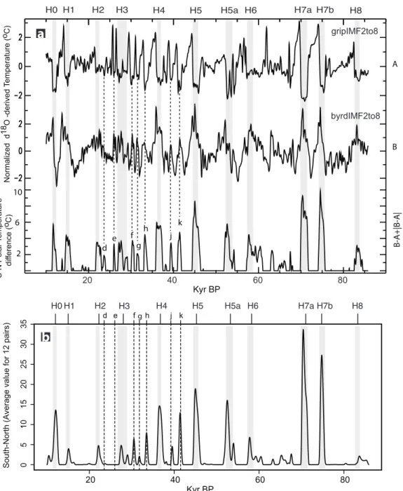
Figure 1.1. Temperature and power calculation for records based on AICC2012 age model [Veres et al., 2013] as well as methane-age-matched records. The southern records from Antarctica have been averaged to reduce local climate variations. From top to bottom for both AICC2012 and age-matched calculation, the y-axis labels are: “Normalized 𝛿/0𝑂-derived
temperature”, “Normalized 𝛿/0𝑂-derived temperature”, “Rectified normalized temperature
gradient”, and “Arrival of energy (arbitrary units)”. d e f g h j k
-6 -2 2 6 -8 -4 0 4 05 10 15 04 0 80 -0.6 0 0.6 -0.4 0.2 01 .0 2. 0 00 .4 0. 8 1. 2 20
0 40 60 80 100 20 40 60 80
H0 H1 H2 H3 H4 H5 H5a H6 H7a H7b H8 H1 H2 H3 H4 H5 H5a H6 H7a H7b
d e f g h j k
AICC2012 Age-matched
NGRIP
Averaged* Antarctica
S-N difference
Power est. DC=2
* average of VOSTOK, EDML, EDC, TALDICE
NGRIP
Averaged* Antarctica
S-N difference
Power est. DC=0.4
* average of VOSTOK, FUJI, DOME C, BYRD
1.3. Results
1.3.1. Polar temperature differences
Figure 1.2. Polar climate S-N temperature gradient. (a) S-N temperature gradient from methane-matched, reconstructed time series GRIP and BYRD compared to the timing of the H events (vertical grey bars, see main text for detail) [Bond and Lotti, 1995; Rashid et al., 2003;
Rasmussen et al., 2003; Hemming, 2004]. The timing of H events and even the timing of minor IRDs (labeled d-k) coincide with times at which the south to north temperature difference is the greatest, as seen in the bottom panel. Intrinsic Mode Functions 2 through 8 were extracted to bandpass-filter the records [Huang et al., 1998]. The S-N temperature difference (B-A) is rectified. (b) S-N temperature differences for all 12 combinations of polar climate time series pairs (three from Greenland, four from Antarctica) with methane based Monte Carlo-matched age model.
20 40 60 80
05 10 15 20 25 30 35
H0 H1 H2 H3 H4 H5 H5a H6 H7a H7b H8
e f h g j k
d Kyr BP South-North (Average value for 12 pairs) gripIMF2to8 byrdIMF2to8 d f g h j k
H0 H1 H2 H3 H4 H5 H5a H6 H7a H7b H8
A B B -A +| B-A | e 10 2 6
Normalized d
18O -derived
Temperature ( o C) S-N Polar Te mperature dif ference ( o C) Kyr BP
20 40 60 80
a
H events are most commonly characterized by massive iceberg discharges of the northern ice sheets carrying coarse sediment to the open sea, occurring near the end of periods of
extremely cold climate as recorded in Greenland’s ice core records. Their influence beyond the region remains uncertain, as do the mechanisms that might trigger these icebergs releases. In most of the literature, the H events are regarded as uniquely Northern Hemisphere events [MacAyeal, 1993; Bond and Lotti, 1995; Marshall and Clarke, 1997; Schulz et al., 2002; MacAyeal et al., 2006; Alvarez-Solas et al., 2010], though their full dynamic history remains incomplete. However, some recent publications have reported climatic events in the equatorial regions and the Southern Hemisphere that were coeval with the H events. For example,
Jennerjahn et al. [2004] published evidence of the southward displacement of the ITCZ
(Intertropical Convergence Zone) in the tropical Atlantic region, with increasing intensity of the northeast trade winds occurring during the H events enhancing the humidity and precipitation in the tropical South America. In addition, Whittaker et al. [2011] published work on speleothems from New Zealand’s Hollywood cave (42°S) that shows abrupt shifts from cold and dry to wet and cool climates occurred at times that coincide with accepted ages of H events in the interval from 73 ka to 11 ka. Further, Sachs and Anderson [2005] suggest that H events may have been connected to sudden ocean productivity increases in the southeast Atlantic and southwest Pacific oceans.
1.3.2. Energy estimation of the polar climate variation
(every 7 to 12 ka) and last a few hundred years [Hemming, 2004], which suggests the action of comparable anomalous, episodic releases of energy. The generally termed IRDs appear to
involve much less energy, as will be shown later. The results shown in Figure 1.2 combined with the polar synchronization hypothesis suggests that a tentative measure of the power (energy rate-of-arrival) involved in the H events is possible.
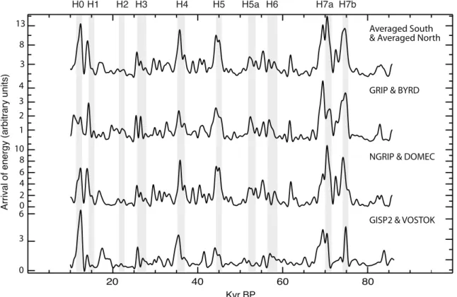
Figure 1.3. Rate of energy arrival (power) for four south-north isotope record pairs. From top to bottom the results are obtained by: all southern records, averaged and squared plus all northern records, averaged and squared; BYRD squared plus GRIP squared; Dome C squared plus NGRIP squared; and VOSTOK squared plus GISP2 squared. The sums, 𝑆(𝑡) 6 = 𝑎(𝑡)6+ 𝑔(𝑡)6, appear
as localized bursts (see text for details). H4 H3
H2
H1 H5 H5a H6 H7a
H0 H7b
Kyr BP
Averaged South & Averaged North
GRIP & BYRD
NGRIP & DOMEC
GISP2 & VOSTOK
20 40 60 80
Arrival of energy (arbitrary units)
The persistent 𝜋 2 phase lock between the polar climate records allows the construction of an analytic function that consisting both climate signals. Having done so, the energy of the system that generates the analytic signal could potentially be estimated following Gabor’s approach [Gabor, 1946]. We construct an analytic signal 𝑠 𝑡 ~𝑎 𝑡 + 𝑖𝑔(𝑡), with magnitude
𝑠(𝑡) = 𝑎(𝑡)6+ 𝑔(𝑡)6, and total energy given by 𝐸 = = 𝑠(𝑡) 6𝑑𝑡
3= (with 𝑎 𝑡 and 𝑔 𝑡 the
same as defined in the introduction session). Thus, the instantaneous power of 𝑠(𝑡) is given by
𝑑𝐸 𝑑𝑡 = 𝑠(𝑡)6~𝑎(𝑡)6+ 𝑔(𝑡)6. This quantity is plotted in Figure 1.3 (see also Figure 1.1).
Heyser [1971] showed experimentally, through the use of sound signals, that the square of the magnitude of an analytic signal (AS) is proportional to the instantaneous rate-of-arrival of the total energy of the real signal. By itself, the square of the original signal, say 𝑎(𝑡)6, would be
proportional to the rate-of-arrival of just one of the components of the energy, and can thus be zero when any component of energy (kinetic or potential) vanishes. In contrast, the square of the magnitude of an AS would be zero only at those times when the total (kinetic plus potential) energy is zero. Notice that, in Figure 1.3, the energy minimum is near zero and that the smaller IRDs do not show as clearly as in the case of polar temperature gradient (Figure 1.2).
The estimated power from the function 𝑠(𝑡)6~𝑎(𝑡)6+ 𝑔(𝑡)6 produces episodic,
1.4. Discussion
The results shown in Figure 1.2 and Figure 1.3 strongly suggest that the occurrence of H events is tied to the coupled climate oscillations of the poles, instead of being a process unique to the Northern Hemisphere or processes happening separately in both hemispheres. Specifically, these figures show that the pulses in energy closely correlated with the H events, as well as with the maxima in the south-north (S-N) temperature gradient, suggesting a strong relationship between the combined polar records and these abrupt events. This bipolar origin of H events would explain why the isotope proxies from Greenland or Antarctica do not show the H events directly, but rather, upon combining the effects of the two polar signals the presence of H events is revealed.
This interaction between the polar climates predicts that the 𝜋 2 phase shift should cause a pulse-like peak of temperature gradient (which here is assumed to be proportional to the
difference between the isotope records from two Polar Regions) based on the assumption that the isotope proxy is a nearly linear function of temperature [Johnsen et al., 1995]) at the times of H5a, H7a, H7b, and H8 (Figure 1.2b), which were discovered more recently than the others [Rashid et al., 2003; Rasmussen et al., 2003]. That is, the polar temperature gradient produces a series of large, isolated pulse-like peaks at ~53, ~72, ~75, and ~83 ka in our results, where these events were eventually found (relative to timings of adjacent IRD events). Further, the timings of the smaller amplitude IRDs, identified by Bond and Lotti [1995] with the letters d-k, are
gradient does not coincide with a potential IRD or H event. Notice that only the (positive) S-N temperature gradient coincides with the IRDs, which is why the temperature gradient time series in Figure 1.2 is rectified.
would then diminish when the condition of the ice sheet is no longer suitable for further calving. In previous research, the H events have either been seen as the cause of the collapse of AMOC [Broecker, 1994, 2003; Timmermann et al., 2005], or as a consequence of the AMOC shutdown [Clark et al., 2007]. However, the relative timing of the North Atlantic subsurface warming, of the maxima in S-N polar temperature gradient, and of the H events may suggest an intervolved relationship that could allow both of the aforementioned arguments to be true. Instead of happening one after another, the H events and the reduction of AMOC may have evolved together. The initial mild reduction (may correspond to the “stadial mode” [Rahmstorf, 2002]) in AMOC observed at the early stage of each stadial contributes to the subsurface warming, with heat coming both from the south and from the reduction in ocean convection in the North Atlantic. When the conditions of both the ice sheets and the subsurface heat are optimal, the initial fresh water input occurs, which, through the aforementioned positive
feedback [Clark et al., 2007], leads to the massive iceberg release that characterizes an H event. At the same time, the massive fresh water input after the initial released may finally collapse the NADW formation and lead to the “off mode” of the AMOC, which is followed by maxima in both polar temperature gradient and subsurface warming.
Despite fresh water input [Shakun et al., 2012] and the many other proposed mechanisms [Ganopolski and Rahmstorf, 2002; Banderas et al., 2014] that may explain the AMOC
distinguishing a pacemaker (or forcing) from the response is very challenging [Clarke et al., 1999].
One of the challenges of modeling the H events is reproducing the phase-lock of the ice-climate coupling [Clarke et al., 1999]. This can be explained via the results of our study, as the behavior of the ice sheets (exemplified by H events and IRDs events) does appear to be coupled with the polar climate synchronization through either polar temperature gradient or energy propagation along the Atlantic basin, either of which may contribute to the coupling of the polar climates. While the role of the S-N polar temperature gradient has been proposed above, the physical processes underlying the energy estimation (Figure 1.3) need further investigation. Despite the analogy between an acoustic signal and the polar climate’s composite signal via the concept of analytic signal, the energy that is calculated here likely results from different
mechanisms than those involved in the acoustic systems. That is, even though the energy maxima reflect nearly all H events, what the energy truly represents in the physical climate system is still unclear.
Under the hypothesis of polar synchronization, each polar climate subsystem potentially affects and is affected by the other, causing both to be nonlinearly transformed (their natural frequencies gradually changing until they lock with each other) by their interaction. It is possible that the polar climates were originally independent, even chaotic, before becoming connected, coupled, climatic oscillations via oceanic heat transfer, potentially channeled by the
REFERENCES
1. Alvarez-Solas, J., S. Charbit, C. Ritz, D. Paillard, G. Ramstein, and C. Dumas (2010), Links between ocean temperature and iceberg discharge during Heinrich events, Nat. Geosci., 3(2), 122–126, doi:10.1038/ngeo752.
2. Alvarez-Solas, J., A. Robinson, M. Montoya, and C. Ritz (2013), Iceberg discharges of the last glacial period driven by oceanic circulation changes, Proc. Natl. Acad. Sci., 110(41), 16350–16354, doi:10.1073/pnas.1306622110.
3. Banderas, R., J. Alvarez-Solas, A. Robinson, and M. Montoya (2014), An
interhemispheric mechanism for glacial abrupt climate change, Clim. Dyn., 1–12, doi:10.1007/s00382-014-2211-8.
4. Barker, S., P. Diz, M. J. Vautravers, J. Pike, G. Knorr, I. R. Hall, and W. S. Broecker (2009), Interhemispheric Atlantic seesaw response during the last deglaciation, Nature, 457(7233), 1097–1102, doi:10.1038/nature07770.
5. Barker, S., G. Knorr, R. L. Edwards, F. Parrenin, A. E. Putnam, L. C. Skinner, E. Wolff, and M. Ziegler (2011), 800,000 Years of Abrupt Climate Variability, Science, 334(6054), 347–351, doi:10.1126/science.1203580.
6. Blunier, T., and E. J. Brook (2001), Timing of Millennial-Scale Climate Change in Antarctica and Greenland During the Last Glacial Period, Science, 291(5501), 109–112, doi:10.1126/science.291.5501.109.
7. Blunier, T. et al. (1998), Asynchrony of Antarctic and Greenland climate change during the last glacial period, Nature, 394(6695), 739–743, doi:10.1038/29447.
8. Bond, G., W. Broecker, S. Johnsen, and J. McManus (1993), Correlations between climate records from North Atlantic sediments and Greenland ice, Nature.
9. Bond, G., B. Kromer, J. Beer, R. Muscheler, M. N. Evans, W. Showers, S. Hoffmann, R. Lotti-Bond, I. Hajdas, and G. Bonani (2001), Persistent Solar Influence on North Atlantic Climate During the Holocene, Science, 294(5549), 2130–2136,
doi:10.1126/science.1065680.
10.Bond, G. C., and R. Lotti (1995), Iceberg Discharges into the North Atlantic on Millennial Time Scales During the Last Glaciation, Science, 267(5200), 1005–1010, doi:10.1126/science.267.5200.1005.
11.Bracewell, R. N. (1986), The Fourier transform and its applications, McGraw-Hill New York.
13.Broecker, W. S. (1998), Paleocean circulation during the Last Deglaciation: A bipolar seesaw?, Paleoceanography, 13(2), 119–121, doi:10.1029/97PA03707.
14.Broecker, W. S. (2003), Does the Trigger for Abrupt Climate Change Reside in the Ocean or in the Atmosphere?, Science, 300(5625), 1519–1522.
15.Clarke, G. K. C., S. J. Marshall, C. Hillaire-Marcel, G. Bilodeau, and C. Veiga-Pires (1999), A Glaciological perspective on Heinrich events, in Geophysical Monograph Series, vol. 112, edited by U. Clark, S. Webb, and D. Keigwin, pp. 243–262, American Geophysical Union, Washington, D. C.
16.Clark, P. U., S. W. Hostetler, N. G. Pisias, A. Schmittner, and K. J. Meissner (2007), Mechanisms for an ∼7-Kyr Climate and Sea-Level Oscillation During Marine Isotope Stage 3, in Ocean Circulation: Mechanisms and Impacts—Past and Future Changes of Meridional Overturning, edited by A. Schmittner, J. C. H. Chiang, and S. R. Hemming, pp. 209–246, American Geophysical Union.
17.Crowley, T. J. (1992), North Atlantic Deep Water cools the southern hemisphere, Paleoceanography, 7(4), 489–497, doi:10.1029/92PA01058.
18.EPICA Community Members (2006), One-to-one coupling of glacial climate variability in Greenland and Antarctica, Nature, 444(7116), 195–198, doi:10.1038/nature05301. 19.Gabor, D. (1946), Theory of communication. Part 1: The analysis of information, J. Inst.
Electr. Eng. - Part III Radio Commun. Eng., 93(26), 429–441, doi:10.1049/ji-3-2.1946.0074.
20.Ganopolski, A., and S. Rahmstorf (2002), Abrupt Glacial Climate Changes due to Stochastic Resonance, Phys. Rev. Lett., 88(3), 038501,
doi:10.1103/PhysRevLett.88.038501.
21.Hemming, S. R. (2004), Heinrich events: Massive late Pleistocene detritus layers of the North Atlantic and their global climate imprint, Rev. Geophys., 42(1), RG1005,
doi:10.1029/2003RG000128.
22.Heyser, R. C. (1971), Determination of Loudspeaker Signal Arrival Times: Part 2, J. Audio Eng. Soc., 19(10), 829–834.
23.Huang, N. E., Z. Shen, S. R. Long, M. C. Wu, H. H. Shih, Q. Zheng, N.-C. Yen, C. C. Tung, and H. H. Liu (1998), The empirical mode decomposition and the Hilbert spectrum for nonlinear and non-stationary time series analysis, Proc. R. Soc. Lond. Ser. Math. Phys. Eng. Sci., 454(1971), 903–995, doi:10.1098/rspa.1998.0193.
25.Johnsen, S. J., D. Dahl-Jensen, W. Dansgaard, and N. Gundestrup (1995), Greenland paleotemperatures derived from GRIP borehole temperature and ice core isotope profiles, Tellus, 47B, 624–629.
26.Knutti, R., J. Flückiger, T. F. Stocker, and A. Timmermann (2004), Strong hemispheric coupling of glacial climate through freshwater discharge and ocean circulation, Nature, 430(7002), 851–856, doi:10.1038/nature02786.
27.MacAyeal, D. R. (1993), Binge/purge oscillations of the Laurentide Ice Sheet as a cause of the North Atlantic’s Heinrich events, Paleoceanography, 8(6), 775–784,
doi:10.1029/93PA02200.
28.MacAyeal, D. R. et al. (2006), Transoceanic wave propagation links iceberg calving margins of Antarctica with storms in tropics and Northern Hemisphere, Geophys. Res. Lett., 33(17), L17502, doi:10.1029/2006GL027235.
29.Marcott, S. A., P. U. Clark, L. Padman, G. P. Klinkhammer, S. R. Springer, Z. Liu, B. L. Otto-Bliesner, A. E. Carlson, A. Ungerer, and J. Padman (2011), Ice-shelf collapse from subsurface warming as a trigger for Heinrich events, Proc. Natl. Acad. Sci., 108(33), 13415–13419.
30.Marshall, S. J., and G. K. C. Clarke (1997), A continuum mixture model of ice stream thermomechanics in the Laurentide Ice Sheet 2. Application to the Hudson Strait Ice Stream, J. Geophys. Res. Solid Earth, 102(B9), 20615–20637, doi:10.1029/97JB01189. 31.Oh, J., E. Reischmann, and J. A. Rial (2014), Polar synchronization and the synchronized
climatic history of Greenland and Antarctica, Quat. Sci. Rev., 83, 129–142, doi:10.1016/j.quascirev.2013.10.025.
32.Rahmstorf, S. (2002), Ocean circulation and climate during the past 120,000 years, Nature, 419(6903), 207–214, doi:10.1038/nature01090.
33.Rashid, H., R. Hesse, and D. J. W. Piper (2003), Evidence for an additional Heinrich event between H5 and H6 in the Labrador Sea, Paleoceanography, 18(4), 1077, doi:10.1029/2003PA000913.
34.Rasmussen, T. L., D. W. Oppo, E. Thomsen, and S. J. Lehman (2003), Deep sea records from the southeast Labrador Sea: Ocean circulation changes and ice-rafting events during the last 160,000 years, Paleoceanography, 18(1), 1018, doi:10.1029/2001PA000736. 35.Rial, J. A. (2012), Synchronization of polar climate variability over the last ice age: in
search of simple rules at the heart of climate’s complexity, Am. J. Sci., 312(4), 417–448, doi:10.2475/04.2012.02.
37.Sachs, J. P., and R. F. Anderson (2005), Increased productivity in the subantarctic ocean during Heinrich events, Nature, 434(7037), 1118–1121, doi:10.1038/nature03544. 38.Schulz, M., A. Paul, and A. Timmermann (2002), Relaxation oscillators in concert: A
framework for climate change at millennial timescales during the late Pleistocene, Geophys. Res. Lett., 29(24), 2193, doi:10.1029/2002GL016144.
39.Shaffer, G., S. M. Olsen, and C. J. Bjerrum (2004), Ocean subsurface warming as a mechanism for coupling Dansgaard-Oeschger climate cycles and ice-rafting events, Geophys. Res. Lett., 31(24), L24202, doi:10.1029/2004GL020968.
40.Shakun, J. D., P. U. Clark, F. He, S. A. Marcott, A. C. Mix, Z. Liu, B. Otto-Bliesner, A. Schmittner, and E. Bard (2012), Global warming preceded by increasing carbon dioxide concentrations during the last deglaciation, Nature, 484(7392), 49–54,
doi:10.1038/nature10915.
41.Steig, E. J. (2006), Climate change: The south–north connection, Nature, 444(7116), 152–153, doi:10.1038/444152a.
42.Steig, E. J., and R. B. Alley (2002), Phase relationships between Antarctic and Greenland climate records, Ann. Glaciol., 35(1), 451–456, doi:10.3189/172756402781817211. 43.Stocker, T. F., and S. J. Johnsen (2003), A minimum thermodynamic model for the
bipolar seesaw, Paleoceanography, 18(4), 1087, doi:10.1029/2003PA000920.
44.Talley, L. D. (1999), Some aspects of ocean heat transport by the shallow, intermediate and deep overturning Circulations, in Mechanisms of Global Climate Change at
Millennial Time Scales, edited by P. U. Clark, R. S. Webb, and L. D. Keigwin, pp. 1–22, American Geophysical Union.
45.Timmermann, A., U. Krebs, F. Justino, H. Goosse, and T. Ivanochko (2005),
Mechanisms for millennial-scale global synchronization during the last glacial period, Paleoceanography, 20(4), PA4008, doi:10.1029/2004PA001090.
46.Veres, D. et al. (2013), The Antarctic ice core chronology (AICC2012): an optimized multi-parameter and multi-site dating approach for the last 120 thousand years, Clim Past, 9(4), 1733–1748, doi:10.5194/cp-9-1733-2013.
47.Whittaker, T. E., C. H. Hendy, and J. C. Hellstrom (2011), Abrupt millennial-scale
changes in intensity of Southern Hemisphere westerly winds during marine isotope stages 2–4, Geology, 39(5), 455–458, doi:10.1130/G31827.1.
CHAPTER 2: POLAR CLIMATE TELECONNECTION OF THE LAST GLACIAL PERIOD: A MODEL INTER-COMPARISON STUDY2
2.1. Introduction
2.1.1. Polar climate teleconnection
Since ice core chronology matching techniques became available, the relationship between polar climates has been of great interest to the paleoclimate community [Bender, 1994; Blunier et al., 1998; Blunier and Brook, 2001]. Although most studies agree on a one-to-one occurrence of warming events during the last glacial period [Schmittner et al., 2003; Blunier and Brook, 2001; EPICA members, 2006], the difference in timing and especially in relative phase of these warming events inspired great interests in investigating the mechanism that connects the climates of the Earth’s Polar Regions. In most paleoclimate studies, data are scarce and limited in resolution, thus models have been extensively used to gain information from data and to help bound the possible speculations on the mechanism. GCM-based experiments have drawn a close relationship between the bipolar teleconnection and the changes in AMOC (Atlantic Meridional Overturning Circulation) strength [Clark et al., 2007; Marcott et al., 2011]. Because of the complexity of the GCMs, it is difficult if not impossible to extract the major underlying physics responsible for the teleconnection. On the other end of the spectrum, conceptual models, with fewer parameters, are ideal in testing the connection mechanism, guiding the interpretation of climate records and informing the GCM experiments.
2 This chapter in under review in the Planetary and Global Change. The original citation is:
Multiple conceptual models have been proposed in the literature based on either the numeric relationship of the polar climate records or their own assumed underlying mechanism of polar climate teleconnection [Schmittner et al., 2003; Stocker and Johnsen et al., 2003; Rial, 2012]. However, as will be detailed later, previous model studies have used different data pre-treatments, and mostly focused on a single direction of record reconstruction. A comprehensive analysis and comparison of the skills of these conceptual models and the models’ robustness against parameter change could provide vital information in guiding future climate
reconstruction work and improve our understanding of coupling mechanism between polar climates. Furthermore, extending the Greenland climate record beyond the length of its ice core record has been of great interest and all the climate models analyzed here have been used for this purpose [Siddall et al., 2006; Barker et al., 2011; Oh et al., 2014]. However, this practice was discouraged by recent discoveries from high resolution climate records, that the Greenland climate record could be decoupled from the rest of the polar climate system possibly due to the extended sea ice formation during some of the lengthened Greenland stadial [Capron et al., 2010; Landais et al., 2015]. Even though current conceptual models all assume a persistent and constant polar climate teleconnection, a comprehensive inter-comparison study of these models, as presented here, will lay the foundation for future investigation of the evolution of the polar climate coupling.
2.1.2. Models
An alternative to the TBS was proposed by Rial [2012], who proposes that a phase
synchronization (PhaseSync) was at play between polar climate oscillations, with the coupling being the energy transfer through intervening ocean and atmosphere; 3) The
Integration/Differentiation model (I/D), the idea of which predates both the TBS and the PhaseSync but is still in active use [Barker et al., 2011], and uses the simple mathematical transform in its name to relate the polar records. These conceptual models, after being verified by the existing records, have also been used to obtained the first order approximation of Greenland climate history beyond the extend of its ice core record [for example, see Siddall et al., 2006; Barker et al., 2011; Oh et al., 2014].
In chronological order, the I/D model was the first conceptual model proposed that accounts for the difference in signal shapes between polar records. It was proposed when it became clear that a simple, linear cross-correlation was unable to capture the different signal shapes between polar records (which also means that a simple lead-lag relationship fails to describe the polar climate connection) [see the discussion in Schmittner et al., 2003; Huybers, 2004; and Schmittner et al., 2004]. The I/D model states that, with proper trend removal and amplitude adjustments, integrating Greenland's ice core temperature record or differentiating the Antarctic temperature record closely reproduces that of the other pole. This idea was revisited in [Rial, 2012], in which it was compared to the idea of phase synchronization. And a numeric differentiation was used to reconstruct an 800 kilo-year (kyr) millennial scale Greenland climate variation [Barker et al., 2011].
between the polar regions [Crowley, 1992]. Conversely, the updated TBS model describes the Southern Ocean as a heat reservoir regulating the climate connection between the South Atlantic and the Antarctic. Based on this assumption, Stocker and Johnsen [2003] proposed that the Antarctic temperature variation can be reproduced from the convolution of the Greenland record with an exponential decay term that represents the damping effect of the Southern Ocean. Through trial and error, Stocker and Johnsen determined the characteristic time for the Southern Ocean was ~1120 years, which was consistent in orders of magnitude with that estimated from climate modeling work. Later, Siddall et al. [2006] applied the inverse of the TBS model to reconstruct Greenland climate history based on the longer Antarctic record.
for most of the last glacial period, which is a strong evidence of synchronization. This phase difference also explains the difference in signal shapes between the polar records.
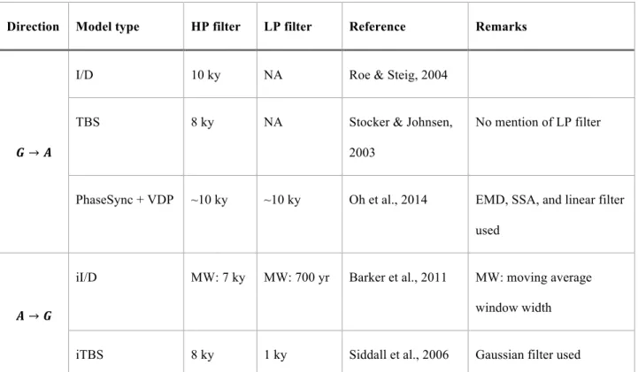
Direction Model type HP filter LP filter Reference Remarks
𝑮 → 𝑨
I/D 10 ky NA Roe & Steig, 2004
TBS 8 ky NA Stocker & Johnsen,
2003
No mention of LP filter
PhaseSync + VDP ~10 ky ~10 ky Oh et al., 2014 EMD, SSA, and linear filter
used
𝑨 → 𝑮
iI/D MW: 7 ky MW: 700 yr Barker et al., 2011 MW: moving average
window width
iTBS 8 ky 1 ky Siddall et al., 2006 Gaussian filter used
Table 2.1. Summary of types of filters and their parameters used in data pre-treatment for the conceptual models discussed in this study. EMD: empirical mode decomposition; SSA: singular spectrum analysis; MW: moving window average; LP: lowpass filter; VDP: Van der Pol
In addition to differences in data pre-treatment, all these models have been inverted to reproduce the records of another pole (the inverted models are denoted by prefixing “i” to their model names). Individual studies on these models often focused on reproducing the climate record for one of the two poles, with no unified test on the modeling skills when reproducing both poles simultaneously. As invertible climate models that represent the two-way
communication of the polar climate system, it is reasonable to expect comparable (or symmetric) skills between reproducing Greenland and Antarctica record. However, there is no existing study that conducted this “two-way” test.
In view of the above questions, in the following work, we first summarize the filter property of each model by extracting their impulse responses, which, in the case of a linear time-invariant system, should fully describe the system’s response to any input. Then we demonstrate and compare the models’ ability to reproduce each polar climate record based on the record from the opposing pole. Lastly, we further test the sensitivity of these models against changing values of data pre-treatment parameters. Siddall et al. [2006] conducted similar test for the iTBS model, where they established that the skill of the iTBS depends on both the model parameter 𝜏 and the filter cutoff frequency 𝜎. To test whether each model gives comparable skills for producing the records of north and south, the sensitivity analysis is carried out in both model directions. 2.2. Methods
2.2.1. Data
such effect from chronology differences by choosing AICC2012 as the proxy chronology, which is considered by most to have the least uncertainty for cross-polar record comparison [Landais et al., 2015].
2.2.2. Data pre-treatment
Past polar climate ice core records exhibit a rich spectrum of oscillatory behaviors, from those in the Milankovitch band to those on the millennial, centennial, or weather-caused scale. The cross-pole one-to-one occurrences of the events studied here are of the millennial scale. Thus, before applying the model, the records were normally filtered to isolate the corresponding frequency band. To achieve this, we applied a 4th order bandpass Butterworth filter with cutoff frequency from 1/8000 to 1/800 yr-1. This effectively suppresses both the direct influence from
the long Milankovitch-scale trend and the high frequency weather-like signal. The filtered records were then normalized, via division by its own standard deviation after mean removal, and tapered to reduce the end effect from the filtering process.
2.2.3. Transfer functions, convolution, and model characteristics
the conceptual polar climate models, the transfer function is the model output when a Dirac function was input to the model. The transfer function is an intrinsic property of each model and is independent of the model input [Oppenheim et al., 1996]. Once obtained, any model response
𝑦(𝑡) can be calculated by convolving the model input 𝑥(𝑡) with its transfer function ℎ(𝑡).
y(t) = x(t) ⊗ h(t)
where the ⊗ denotes the convolution operation.
Once calculated, the transfer function of each model was Fourier transformed to obtain the amplitude and phase responses. The transfer functions and their frequency domain
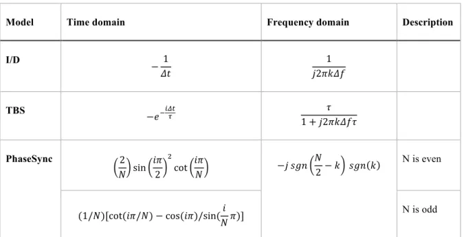
Model Time domain Frequency domain Description
I/D
− 1 𝛥𝑡
1 𝑗2𝜋𝑘𝛥𝑓
TBS
−𝑒3YZ[\ 𝜏
1 + 𝑗2𝜋𝑘𝛥𝑓𝜏
PhaseSync 2
𝑁 sin 𝑖𝜋
2 6
cot 𝑖𝜋
𝑁 −𝑗 𝑠𝑔𝑛
𝑁
2− 𝑘 𝑠𝑔𝑛 𝑘
N is even
(1/𝑁)[cot(𝑖𝜋/𝑁) − cos(𝑖𝜋)/sin(𝑖 𝑁𝜋)]
N is odd
Table 2.2. Transfer functions for the conceptual models. For the time domain representation, 𝑖 is the index number ranging from 1 to the length of the record N. For the frequency domain
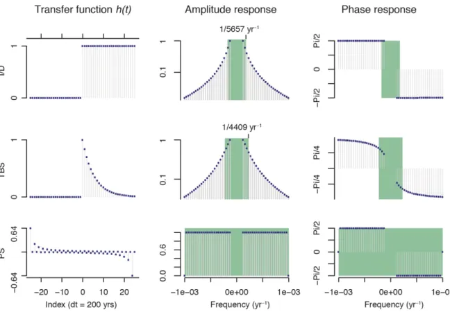
Figure 2.1. Model characteristics. Left column: time domain representations of the model transfer functions. 𝜏 = 1120 years is used to calculate the transfer function for TBS model. Middle column: amplitude responses of the transfer functions. The green portion spans the passband of the amplitude responses and the values of the corner frequencies are shown for the I/D and TBS models. Right column: phase responses of the transfer functions. The I/D and PhaseSync models both have a 𝜋/2 phase response. Initial Butterworth filters has removed frequencies lower than
1/8000 yr-1, the effect of which is represented as the gap at the low frequencies of the amplitude
2.3. Results
2.3.1. Comparison of amplitude and phase responses
As revealed in Figure 2.1, both the I/D and TBS models intrinsically function as low-pass filters, which pass the low frequency part of the model input while suppressing the high
frequency part. While the two models become identical when 𝜏 goes to infinity, when the 𝜏 is in the range of hundreds of years, theoretical cutoff frequencies of the two filters have one order of magnitude difference, such that the I/D model suppresses the high frequency further than the TBS model. However, the actual implementations of the I/D and TBS models yield almost identical results (see simulations in Figure 2.2a). This similarity is caused by removal of the low frequency portion of the record, where the two filters differ the most, in the data pre-treatment step that was meant to isolate the millennial frequencies. The effect from this initial filter is shown in Figure 2.1 as the gap at the low frequency region of the amplitude and phase responses, while the green rectangle represents the passing band of each model. The simulation in Figure 2.2a results from sequentially applying the Butterworth bandpass filter and the polar
teleconnection models, showing their combined effect. This combined effect further reveals that the I/D and TBS models share very similar structure in their amplitude responses (see Figure 2.1 and Figure. S2.2). The results from the PhaseSync model, represented by Hilbert transformation, show that the model functions as an all pass operation that does not change the amplitude of any frequency. However, it does apply a 𝜋/2 phase shift to the model input, which, in this respect, is the same as the I/D model.
2.3.2. Modeling Antarctic record
model outputs are compared to the tapered, normalized, and filtered actual records by calculating the Pearson correlation coefficient between them. The model formulas and their inverted
versions can be found in Appendix 2.
We first applied the models to simulate the Antarctic EDC record from that of
Greenland's NGRIP (Figure 2.2a). The cross-correlation function (CCF) in Figure 2.2c shows that all three models yielded similar reconstructions, and they all closely reproduce the target Antarctic EDC record with maximum correlation values of 0.76, 0.73, 0.73 for the I/D, TBS, and the PhaseSync model respectively. The lags that correspond to maximum correlation in Figure 2.2c are less than 200 years and are well within the chronology uncertainties of the record. However, the actual EDC 𝛿𝐷 has distinctive structures that are not replicated by any of the models. For example, the actual record showed complex peak structures (see double/multiple peaks at 54, 39, and 15 kya in EDC in Figure 2.2a). None of the models investigated here were able to replicate these structures. These complex peak structures in the EDC record may result from local climate variations that were independent from the polar climate teleconnection. 2.3.3. Modeling Greenland record
actual NGRIP record. Also, the lead-lag relations between model results and the target NGRIP record are consistent (Figure 2.2d), with the model results lagged behind the Greenland record by about 170 years on average (232 years for the iTBS model, 150 years for the iPhaseSync model, and 134 for the iI/D model). Even though this lag may be the consequence of systematic
chronology uncertainty, it is consistent with the recent discovery based on WAIS-Divide ice core, which showed abrupt warmings in Greenland on average led those in the Antarctica by
2.3.4. Model skill and robustness against data pre-treatment
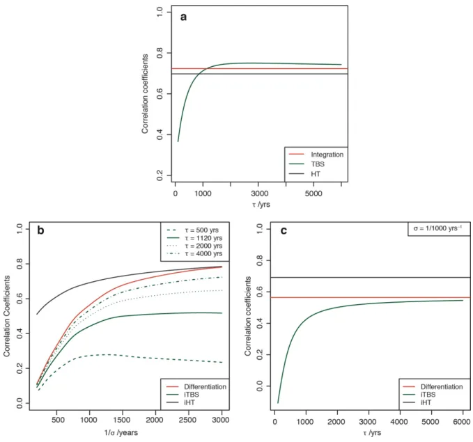
In order to estimate the skills of these models in reproducing the Antarctic record, we calculated the Pearson correlation coefficients between the simulations and the EDC 𝛿𝐷 record. As the result of the TBS model depends on the value of the 𝜏 parameter, we simulated the Antarctic record using different 𝜏 ranging from 0 to 6000 yrs and plotted the correlation as a function of 𝜏 (Figure 2.3a). The correlation coefficients for the other two models are also shown for comparison. The result shows that the skill of the TBS becomes less sensitive to the 𝜏 value beyond ~1000 yrs, suggesting one might need extra justification for choosing 𝜏 value in this range. In addition, the tendency of convergence between the TBS and I/D models can be observed from Figure 2.3a with increasing value of 𝜏.
Unlike reproducing the Antarctic record, previous studies have shown that the skill of the iTBS model is very sensitive to the change of the smoothing parameter in the data pre-treatment stage, due to the tendency of the iTBS and iI/D models to amplify high frequency components. Here, this smoothing factor is controlled by the lowpass cutoff frequency of the Butterworth filter (denoted by 𝜎). To determine the robustness of model skills against changes in this parameter, we have varied the value of 𝜎 in the interval between 1/3000 to 1/200 yrs-1 and
plotted the corresponding model skills in Figure 2.3b for each inverted model. We also fixed the
may be due to the differences in the chronologies used. Since we are using the same record pair and the same chronology consistently throughout this study, such effect is minimized.
Figure 2.3. Model skills against change in data-pretreatment parameters. a. Model skills in reproducing the Antarctic record measured in the Pearson correlation coefficients between the simulations and the actual EDC record. The skill of the TBS model depends on the value of 𝜏. b-c. Model skills represented by correlation coefficients between the simulations and the actual NGRIP record. b. The dependence of model skill on the corner frequency 𝜎 of the low-pass filter while fixing 𝜏 at four different values ranging from 500 to 6000 yrs. c. The dependence of model skill on the time constant 𝜏 from the iTBS model while fixing 𝜎 at 1/1000 yr-1. HT and iHT
2.4. Discussion
The models investigated in this study represent our current conceptual understanding of the teleconnection between the polar climates. Of the three models investigated, the I/D and TBS models share many numeric properties, which can be explained by the fact that the latter
converges to the former model when its 𝜏 parameter approaches infinity. Both behave as low-pass/high-pass filters in the Greenland-to-Antarctica/Antarctica-to-Greenland directions,
respectively. Furthermore, their skills are both asymmetric and sensitive to the inclusion of high frequency content in the model input (Figure 2.4). While the TBS and I/D models selectively suppress the high frequency content of the input (or the low frequency with their inverse), the PhaseSync model passes all the frequency content. Because of this property, the PhaseSync model is the most robust one against inclusion of noise or high frequency climate variations in the model input, requiring the least tuning of the data. And in contrast to I/D and TBS models, its skill is directionally symmetric (that is, comparable skills under the same data pre-treatment) in reproducing polar records.
Both the TBS and PhaseSync models were originally built upon assumptions of specific physical processes. The TBS model attributed the polar climates coupling to the heat transfer in the Atlantic Ocean. In its original form, Stocker and Johnsen [2003] derived the Antarctic temperature evolution as the result of heat transfer from the north, thus a north-to-south one-way coupling. In contrast, the phase synchronization model requires a bi-directional coupling
between the polar climate oscillations. Although it does not inherently restrict the exact form of coupling, the intervening oceanic and atmospheric processes provide various potential
Saltzman [1982; 2002]. In this specific modeling setting, the polar climate oscillators, being coupled through the difference in the mean temperature of the ocean between the northern and southern hemispheres, is able to reproduce both the characteristics of polar records and their coupling. This provides a relationship between the poles that involves the mutual interaction between the two Polar Regions, an appealing mechanism based in well-known properties of nonlinear coupled synchronizing oscillators. As a possible signal pathway, the cross-pole, oceanic, heat transfer described in the TBS model could potentially contribute to the coupling of the polar climate oscillations.
In conclusion, polar teleconnection conceptual models not only provide a mathematical description of the relationship between ice core records, they also suggest potential physical coupling mechanisms. Here, we have analyzed the skills of three teleconnection models and discussed their underlying physical mechanisms. We found that the PhaseSync model outperforms the I/D and TBS models for a wide range of parameter values, accurately
reproducing climate records from both poles. We introduced the merits of phase synchronization as a framework for the polar climate teleconnection and suggest that the oceanic heat transfer as described in the thermal bipolar seesaw conceptual model could be integrated into the
REFERENCES
1. Barker, S., G. Knorr, R. L. Edwards, F. Parrenin, A. E. Putnam, L. C. Skinner, E. W. Wolff, and M. Ziegler (2011), 800,000 years of abrupt climate variability, Science, 334(6054), 347– 351, doi:10.1126/science.1203580.
2. Bender, M., T. Sowers, M.-L. Dickson, J. Orchardo, P. Grootes, P. A. Mayewski, and D. A. Meese (1994), Climate correlations between Greenland and Antarctica during the past 100,000 years, Nature, 372(6507), 663–666, doi:10.1038/372663a0.
3. Blunier, T. et al. (1998), Asynchrony of Antarctic and Greenland climate change during the last glacial period, Nature, 394(6695), 739–743, doi:10.1038/29447.
4. Blunier, T., and E. J. Brook (2001), Timing of millennial-scale climate change in Antarctica and Greenland during the last glacial period, 291(5501), 109–112,
doi:10.1126/science.291.5501.109.
5. Buizert, C. et al. (2015), Precise interpolar phasing of abrupt climate change during the last ice age, Nature, 520(7549), 661–U169, doi:10.1038/nature14401.
6. Capron, E., A. Landais, J. Chappellaz, A. Schilt, and D. Buiron (2010), Millennial and sub-millennial scale climatic variations recorded in polar ice cores over the last glacial period,, doi:10.1029/2003PA000920/full.
7. Clark, P. U., S. W. Hostetler, N. G. Pisias, A. Schmittner, and K. J. Meissner (2007), Mechanisms for an∼ 7-kyr climate and sea-level oscillation during marine isotope stage 3, Geophys. Monogr. Ser., 173, 209–246, doi:10.1029/173GM15.
8. Crowley, T. J. (1992), North Atlantic Deep Water cools the southern hemisphere, Paleoceanography, 7(4), 489–497, doi:10.1029/92PA01058.
9. Fradkov, A. L., and B. Andrievsky (2007), Synchronization and phase relations in the motion of two-pendulum system, International Journal of Non-Linear Mechanics, 42(6), 895–901, doi:10.1016/j.ijnonlinmec.2007.03.016.
10.Huybers, P. (2004), Comments on “Coupling of the hemispheres in observations and simulations of glacial climate change” by A. Schmittner, O.A. Saenko, and A.J. Weaver, Quaternary Science Reviews, 23(1-2), 207–210, doi:10.1016/j.quascirev.2003.08.001. 11.Huygens, C. (1986), Christiaan Huygens' the pendulum clock, or, Geometrical
demonstrations concerning the motion of pendula as applied to clocks, Iowa State Pr. 12.Landais, A. et al. (2015), A review of the bipolar see–saw from synchronized and high
13.Lisiecki, L. E., and M. E. Raymo (2009), Diachronous benthic δ18O responses during late Pleistocene terminations, Paleoceanography, 24(3), doi:10.1029/2009PA001732.
14.Marcott, S. A. et al. (2011), Ice-shelf collapse from subsurface warming as a trigger for Heinrich events, PNAS, 108(33), 13415–13419, doi:10.1073/pnas.1104772108.
15.Oh, J., E. Reischmann, and J. A. Rial (2014), Polar synchronization and the synchronized climatic history of Greenland and Antarctica, Quaternary Science Reviews, 83, 129–142,
doi:10.1016/j.quascirev.2013.10.025.
16.Oppenheim, A. V., A. S. Willsky, and S. H. Nawab (1996), Signals and Systems (2nd Ed.), Prentice-Hall, Inc., Upper Saddle River, NJ, USA.
17.Pikovsky, A., M. Rosenblum, and J. Kurths (2001), Synchronization. Cambridge Nonlinear Science Series 12.
18.Rial, J. A. (2012), Synchronization of polar climate variability over the last ice age: in search of simple rules at the heart of climate's complexity, Am J Sci, 312(4), 417–448,
doi:10.2475/04.2012.02.
19.Roe, G. H., and E. J. Steig (2004), Characterization of Millennial-Scale Climate Variability, Journal of Climate, 17(10), 1929–1944,
doi:10.1175/1520-0442(2004)017<1929:COMCV>2.0.CO;2.
20.Saltzman, B. (1982), Stochastically-driven climatic fluctuations in the sea-ice, ocean temperature, CO2 feedback system, Tellus.
21.Saltzman, B. (2002), Dynamical Paleoclimatology, Academic Press.
22.Schmittner, A., O. A. Saenko, and A. J. Weaver (2003), Coupling of the hemispheres in observations and simulations of glacial climate change, Quaternary Science Reviews, 22(5-7), 659–671, doi:10.1016/S0277-3791(02)00184-1.
23.Schmittner, A., O. SAENKO, and A. WEAVER (2004), Response to the comments by Peter Huybers, Quaternary Science Reviews, 23(1-2), 210–212,
doi:10.1016/j.quascirev.2003.08.002.
24.Siddall, M., T. F. Stocker, T. Blunier, R. Spahni, J. F. McManus, and E. Bard (2006), Using a maximum simplicity paleoclimate model to simulate millennial variability during the last four glacial periods, Quaternary Science Reviews, 25(23-24), 3185–3197,
doi:10.1016/j.quascirev.2005.12.014.
27.Stocker, T. F., and S. J. JOHNSEN (2003), A minimum thermodynamic model for the bipolar seesaw, Paleoceanography, 18(4), 1087–n/a, doi:10.1029/2003pa000920.
28.Veres, D. et al. (2013), The Antarctic ice core chronology (AICC2012): an optimized multi-parameter and multi-site dating approach for the last 120 thousand years, Clim. Past, 9(4), 1733–1748, doi:10.5194/cp-9-1733-2013.
29.Wunsch, C. (2003), Greenland—Antarctic phase relations and millennial time-scale climate fluctuations in the Greenland ice-cores, Quaternary Science Reviews, 22(15-17), 1631–1646,
doi:10.1016/S0277-3791(03)00152-5.
CHAPTER 3: POLAR CLIMATES PHASE COHERENCE THROUGH THE LAST GLACIAL PERIOD
3.1. Introduction
The polar climate proxy records from Greenland and Antarctica have been known to have a one-to-one recurring of warming events during the last glacial period [EPICA Community Members, 2006]. However, it is well known that the proxy records (temperature proxy, either
𝛿/0𝑂 or 𝛿𝐷) between the two poles do not share a simple lead-lag relation. Instead, a stable
phase relationship centered about 𝜋 2 between them has been proposed and embedded in various conceptual models that attempt to characterize their relationship. Rial [2012] has
conducted a systematic analysis of polar phase difference, demonstrating that the polar climates have been in a state of 𝜋 2 phase synchronization for the duration between 10-90 ka (kilo-years before present). The 𝜋 2 phase relation also happens to be embedded in other models that describe the relation between the polar proxy records (see [Schmittner et al., 2003; Huybers, 2004; Steig, 2006], and analysis presented in Chapter 2). According to Rial [2012], a 𝜋 2 phase difference naturally accounts for the difference in the shapes of the warming events. The success in describing the polar climate relationship with simple conceptual models has led to multiple attempts to reconstruct the Greenland climate history beyond the length of the ice core
record[Siddall et al., 2006; Barker et al., 2011].
validity of this assumption and, more importantly, to be able to provide a first degree estimation of the uncertainty for the reconstructed polar climate, an investigation of the robustness of the polar phase relationship is needed. Moreover, recent high resolution polar ice core proxies have revealed periods of decoupling between the Greenland climate and the low latitude hydrological variations in the sub-millennial scale, challenging the role of the Greenland record as the
indicator for oceanic processes in the North Atlantic [Guillevic et al., 2014; Landais et al., 2015]. A detailed polar phase relationship investigation will aide in detecting periods of weak
coherence, if any, thus revealing if decoupling also occurs in the millennial band of climate variation.
With the help of recent developments in unified cross-pole chronology that greatly reduced the timing uncertainty of the millennial scale events [see like Veres et al., 2013], we quantify the millennial frequency band phase characteristics between the polar ice core water isotopes proxy data (namely, 𝛿/0𝑂 and 𝛿𝐷). Our results confirm the robustness of the 𝜋 2 phase
relationship, which persists through majority of the last glacial period (10 – 110 ka). At the same time, we also identify instances of weak coherence, during which the phase differences between the records change abruptly and behave near randomly with a much weaker coherence. Since the strength of coherence describes the communication of climatic signals between the polar regions, the variation may involve changing circulation patterns in the intervening oceans or atmosphere. Indeed, despite the low sampling intensity towards the older section last glacial period, we demonstrate that the weak coherence tends to coincide in timing with periods of reduced/ceased ocean mixing, as revealed by the plateaus in the 𝜀mn tracer records (defined as the /op𝑁𝑑//oo𝑁𝑑
coupled-relaxation oscillator, in which we determined the critical role of the ocean heat exchange in sustaining a coherent phase relation between polar records. We then further attribute the changes in the polar phase coherence to changes in the summer insolation forcing at 65°N latitude, suggesting the insolation may have been regulating the polar climate communication through the last glacial period.
We have divided our text into following parts. In the results section, we first demonstrate the close relationship between the insolation curve and the coherence curve, and then show the possible connection between the strength of the coherence to the strength of the ocean
circulation. The results section is followed by the discussion, where we discussed in detail the implication of the linkage between insolation, coherence, and the ocean circulation strength. In the final methods section, we elaborate on the steps we take to obtain the mean phase coherence curve as well as the details in the conceptual model applied in this study.
3.2. Results
3.2.1. Phase coherence and its relationship with insolation forcing
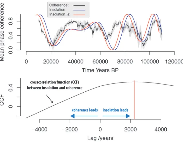
The windowed mean phase coherence reveals the variation in phase coherence between polar climate records. During the last glacial period, the phase coherence has gone through stages of strong and weak coherence, with relatively smooth transitions that are likely due to the
Figure 3.1. Polar phase coherence over the last glacial period. Upper panel. Black line: average phase coherence between the NGIRP 𝛿/0𝑂 and the 𝛿/0𝑂 or 𝛿𝐷 from four Antarctica ice cores;
Insolation forcing has long been recognized as one of the most important external
forcings of the climate on the Earth. The specific summer insolation at mid-latitude (here we take the 65°N; the Matlab code we used to calculate insolation forcing is from Huybers [2006]) has been consistently used in the interpretation of climate records as it has strong influence over the growth of the mid-latitude ice sheet. We have discovered a close connection between polar climate phase coherence and the insolation variation at 65°N (Figure 3.1a). The strong
connection is evidenced by observing the two curves together, where the weak coherence tends to follow the period of reduced insolation forcing (noticing the direction of time is to the left). This relationship is robust as it is able explain all three instances of weak coherence with minima in the insolation. Vice versa, strong and intermediate insolation forcing coincide with strong polar coherence that has been maintained for majority of the last glacial period. A further cross-correlation function has been applied between the insolation and the coherence curve (Figure 3.1b). The result not only confirms the presence of a lagged correlation between them, but also shows that the insolation, on average, leads the coherence by about 2000 years.
3.2.2. Phase coherence and its connection with rate of deep ocean mixing
during which periods millennial scale warming events are found lacking. Concomitantly, these periods also see a reduction in the mixing of water masses between North Atlantic Deep Water (NADW) and Antarctic Bottom Water (AABW) in 𝜀mn records from both the southeastern
Figure 3.2. Polar phase coherence and the rate of ocean mixing. From top to bottom. 1) NGRIP
𝛿/0𝑂 record [Veres et al., 2013]; 2) Mean phase coherence between NGRIP and for Antarctica
ice core records (EDML, EDC, VOSTOK, TALDICE) calculated with a moving window of width 6000 years; 3) The same to 2) but with window width 10 thousand years; 4) 𝜀mn composite record from southeastern Atlantic sediment core RC11-83/TN057-21 [Piotrowski et al., 2005]; 5)
𝜀mn record from Indian Ocean sediment core SK129 [Wilson et al., 2015]; 6) EDML 𝛿/0𝑂
3.2.3. The oceanic control of the simulated polar climate phase coherence
Finally, to test our hypothesis that the ocean circulation strength is able to influence the polar phase coherence, we have utilized a conceptual model built upon the coupling of two nonlinear relaxation oscillators. Each oscillator is a Van der Pol oscillator and is able to reproduce both the characteristic saw-tooth shape of the Greenland isotope record and the triangular Antarctic record [Rial, 2012; Oh et al., 2014]. The same type of model has been frequently used in paleoclimate research to simulate the 100,000 year late Pleistocene glaciation [Saltzman et al., 1981] and the 𝜋 2 phase relation between polar records [Rial, 2012]. The two coupled oscillators are assigned their roles as representing the north (Greenland, oscillator 1) and the south (the Antarctica, oscillator 2), respectively. In each oscillator, the variations in the sea ice extent (idealized as the latitude of the sea ice margin towards equator) and the mean ocean temperature are calculated. The two oscillators are coupled through the difference in both mean ocean temperature (reactive coupling) and rate of mean ocean temperature change (dissipative coupling) with parameters 𝑞/ and 𝑞6 controlling the strength of dissipative coupling and reactive coupling, respectively.
To investigate the effect of coupling strength on the final phase coherence between the simulated polar records, each coupling parameter has been isolated (by assuming the other coupling strength zero) and incrementally increased. For each coupling strength, the cVDP model has been run for 100 kilo-year (ky) five times, each with a random set of initial conditions for {u1, u2, u3, u4} (see model details in the following Methods section). The length of the
Figure 3.3. The influence from the coupling parameters on the phase synchronization between the two oscillators. The natural frequencies of oscillator 1 and 2 are 1/1500 year-1 and 1/3000 year-1. When testing 𝑞/, the value of 𝑞6 was kept 0. The same is true when testing 𝑞6. For each 𝑞
From the testing results (Figure 3.3), we conclude that, given sufficiently large coupling strength, both coupling parameters 𝑞/ and 𝑞6 can independently achieve phase synchronization between the two oscillators. It is also important to notice that, even with different assigned natural frequencies between oscillator 1 (1 1500 year-1) and oscillator 2 (1 3000 year-1), synchronization can be achieved with sufficiently strong coupling through increasing either 𝑞/ or
𝑞6. However, when synchronization is obtained, 𝑞/ and 𝑞6 result in different phase difference. With increasing 𝑞/, the phase difference between oscillator 1 and oscillator 2 stabilizes at 𝜋 2. On the contrary. Increasing 𝑞6 lead to a − 𝜋 2 phase difference. From the polar records, we
learnt that the phase difference is centered around 𝜋 2. If we assume the model gives a
reasonably good representation of the large-scale interactions between the polar climates through the intervening ocean, then the consistencies between the phase relationships of the ice core records and the simulations controlled by 𝑞/ could suggest that the difference in the rate of change in the mean ocean temperature (dissipative coupling) between respective oceans plays a greater role. To put this in terms of the actual physical system, the model results show that it is not the difference in absolute ocean temperature, but rather the asymmetric heat (rate of change of temperature) distribution/transfer between the north and south which plays a key role in regulating polar climate connection.
3.3. Discussion
![Figure 1.1. Temperature and power calculation for records based on AICC2012 age model [Veres et al., 2013] as well as methane-age-matched records](https://thumb-us.123doks.com/thumbv2/123dok_us/8286815.2194441/15.918.109.751.450.746/figure-temperature-calculation-records-veres-methane-matched-records.webp)