EFFICIENT WAVE-BASED SOUND PROPAGATION AND OPTIMIZATION FOR COMPUTER-AIDED DESIGN
Nicolas M. Morales
A dissertation submitted to the faculty of the University of North Carolina at Chapel Hill in partial fulfillment of the requirements for the degree of Doctor of Philosophy in the Department of Computer Science.
Chapel Hill 2018
ABSTRACT
Nicolas M. Morales: Efficient Wave-based Sound Propagation and Optimization for Computer-Aided Design (Under the direction of Dinesh Manocha)
Acoustic phenomena have a large impact on our everyday lives, from influencing our enjoyment of music in a concert hall, to affecting our concentration at school or work, to potentially negatively impacting our health through deafening noises. The sound that reaches our ears is absorbed, reflected, and filtered by the shape, topology, and materials present in the environment. However, many computer simulation techniques for solving these sound propagation problems are either computationally expensive or inaccurate. Additionally, the costs of some methods are dramatically increased in design optimization processes in which several iterations of sound propagation evaluation are necessary.
The primary goal of this dissertation is to present techniques for efficiently solving the sound propagation problem and related optimization problems for computer-aided design. First, we propose a parallel method for solving large acoustic propagation problems, scalable to tens of thousands of cores. Second, we present two novel techniques for optimizing certain acoustic characteristics such as reverberation time or sound clarity using wave-based sound propagation. Finally, we show how hybrid sound propagation algorithms can be used to improve the performance of acoustic optimization problems and present two algorithms for noise minimization and speech intelligibility improvement that use this hybrid approach.
ACKNOWLEDGMENTS
The research in this dissertation could not have been done without the help and support of others. First, I would like to thank my coauthors on the various papers I present. These include Ravish Mehra, Vivek Chavda, Zhenyu Tang, and of course my advisor, Dinesh Manocha. On many of these papers, I benefited from the knowledge and experience of Abhinav Golas, Alok Meshram, Atul Rungta, Allan Porterfield, Carl Schissler, and Auston Sterling, all who had important suggestions and critiques.
Aside from these technical contributions, I never would have made it through grad school without my friends and family. My parents have always encouraged me to do my best, and they were always supportive during the highs and lows of my graduate career. I would also like to thank all my friends. Their support during my work on this dissertation was essential.
TABLE OF CONTENTS
LIST OF TABLES . . . x
LIST OF FIGURES . . . xi
1 INTRODUCTION . . . 1
1.1 Models for Sound Propagation . . . 1
1.2 Acoustic Optimization . . . 4
1.3 Challenges . . . 6
1.4 Thesis Statement . . . 9
1.5 Main Contributions . . . 9
1.5.1 Parallel Wave-Based Sound Propagation . . . 10
1.5.2 Wave-Based Techniques for Acoustic Material Optimization . . . 11
1.5.3 Hybrid Techniques for Acoustic Optimization . . . 12
1.6 Organization . . . 13
2 BACKGROUND . . . 14
2.1 Sound Propagation . . . 14
2.1.1 Geometric Methods . . . 14
2.1.2 Wave-Based Sound Propagation . . . 15
2.2 Adaptive Rectangular Decomposition . . . 16
2.2.1 Pressure Field Computation . . . 16
2.2.2 Interface Handling . . . 17
2.2.3 ARD computational pipeline . . . 18
3.1 Previous work . . . 21
3.1.1 Parallel wave-based solvers . . . 21
3.1.2 Domain decomposition . . . 22
3.1.3 Low dispersion acoustic solvers . . . 22
3.2 Parallel ARD . . . 23
3.2.1 Partition and Interface Ownership . . . 24
3.2.2 Parallel Algorithm . . . 24
3.2.3 Efficient Load Balancing . . . 25
3.3 Scaling to Large Clusters . . . 26
3.3.1 Communication efficiency . . . 27
3.3.2 Load balancing and numerical stability . . . 29
3.3.3 Interface and PML computation . . . 29
3.3.4 MPARD Pipeline . . . 30
3.3.4.1 Voxelization . . . 31
3.3.4.2 Decomposition . . . 31
3.3.4.3 Core allocation and subdomain splitting . . . 31
3.3.4.4 Interface and PML preprocessing . . . 32
3.4 Results and analysis . . . 32
3.4.1 Scalability results . . . 34
3.4.2 Load Balancing . . . 34
3.4.3 Communication Costs . . . 37
3.4.4 Error and Validation . . . 39
3.4.5 Comparisons and benefits . . . 40
3.5 Conclusion and future work . . . 42
4 Efficient Wave-Based Acoustic Material Design Optimization . . . 43
4.1 Prior Work . . . 44
4.1.2 Acoustic Optimization . . . 45
4.1.2.1 Object Models . . . 46
4.1.2.2 Spatial Models . . . 46
4.2 Acoustic Metrics . . . 48
4.2.1 Strength and Clarity . . . 48
4.2.2 Reverberation Time . . . 48
4.3 Gradient-Based Acoustic Optimization and Sensitivity Analysis . . . 49
4.3.1 Acoustic Optimization . . . 50
4.3.2 Sensitivity Analysis . . . 52
4.3.3 Computing the Pressure Field Gradient . . . 53
4.3.4 Automatic Differentiation (AD) . . . 55
4.4 Results and Analysis of Gradient-Based Acoustic Optimization . . . 57
4.4.1 Benchmarks . . . 57
4.4.1.1 Acoustic Materials . . . 57
4.4.1.2 Acoustic Metrics and the Impulse Response . . . 58
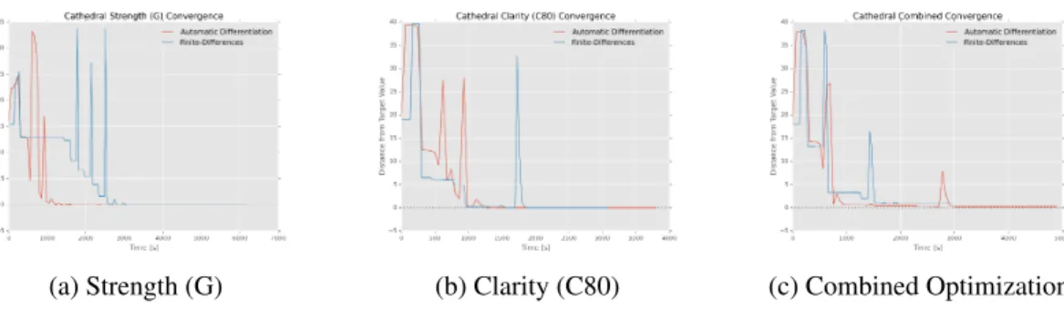
4.4.2 Convergence . . . 58
4.4.3 Optimization Results . . . 59
4.4.4 Analysis . . . 60
4.5 Discrete material optimization for wave-based acoustic design . . . 62
4.5.1 The Objective Function . . . 63
4.5.2 Optimization Approach . . . 64
4.5.2.1 Simulated Annealing . . . 65
4.5.2.2 Reducing Iteration Cost . . . 67
4.5.3 Acoustic Materials. . . 68
4.6 Results and Validation of Discrete Material Optimization . . . 68
4.6.1 Experimental Setup . . . 69
4.6.3.1 Early-Cutoff and Adaptive Initial Temperature . . . 72
4.6.4 Performance . . . 73
4.6.5 Impulse Responses . . . 73
4.6.6 Full-field Results . . . 77
4.6.7 Validation . . . 77
4.7 Conclusion and Future Work . . . 81
5 Hybrid Approaches for Noise Minimization and Improving Speech Intelligibility . . . 83
5.1 Hybrid Propagation . . . 85
5.2 Noise Control and Optimization. . . 87
5.2.1 Prior Work . . . 89
5.2.2 Computing Noise Exposure . . . 90
5.3 Optimizing Source Placement for Noise Minimization Using Hybrid Acoustic Simulation . . . 92
5.3.1 Source configuration . . . 94
5.3.2 Sound Source Clustering . . . 94
5.3.3 Simulated Annealing . . . 96
5.3.3.1 Simulated Annealing State . . . 97
5.3.4 Impulse Response Caching . . . 97
5.4 Results of Noise Minimization . . . 99
5.4.1 Performance . . . 100
5.4.2 Noise Minimization . . . 101
5.4.3 Error Analysis . . . 105
5.5 Minimizing Noise in Speech Recognition Applications . . . 106
5.5.1 Prior Work . . . 107
5.6 Receiver Placement Optimization . . . 108
5.6.1 Speech Transmission Index . . . 109
5.6.2 Our Optimization Algorithm . . . 109
5.8 Conclusion and Future Work . . . 113
5.8.1 Noise Minimization . . . 113
5.8.2 Speech Intelligibility Improvement . . . 114
6 SUMMARY AND CONCLUSIONS . . . 115
6.1 Summary of Results . . . 115
6.2 Limitations . . . 116
6.3 Future Work . . . 117
LIST OF TABLES
3.1 Comparison between different ARD techniques include MPARD, the method we introduce. . . 23
3.2 Dimensions and complexity of the scenes used in our experiments. . . 32
4.1 Summary of the various benchmark scenes. . . 57
4.2 The various starting and ending material values for optimization. . . 59
4.3 Volumes and number of material segments for each scene. . . 68
4.4 Target values and weights for the single-metric optimization optimization. . . 70
4.5 Summary of the multiobjective optimization experiments. . . 71
4.6 Running time and number of iterations for our experiments including single-target G, C80, and RT60 experiments and one experiment using a multi-objective target for multiple metrics. . . 74
4.7 Comparison of discrete material optimization using ARD and using Sabine. . . 81
5.1 We highlight the benchmark scenes, their sound sources, the minimized noise level, and the clustering ratio. . . 100
5.2 The total running time of each scene along with the number of cells used for the ARD algorithm and the number of triangles in the CAD models corresponding to our benchmarks. . . 101
5.3 Notation and symbols used in our acoustic solver and optimization algorithm. . . 108
5.4 STI scale and qualification. . . 111
LIST OF FIGURES
1.1 Plots showing permissible noise exposure and the noise weighting curves
com-monly used in regulatory agencies such as OSHA. . . 5
1.2 Side-by-side comparison of how speech intelligibility at the receiver location of an ASR device can change according to its location. . . 6
1.3 A top-down slice of the simulation domain of the ˇSibenik Cathedral. . . 7
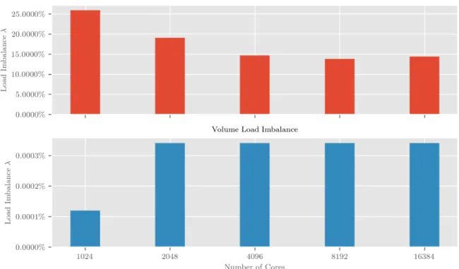
1.4 Scalability of the MPARD technique from 1024 to 16384 cores on the 5 kHz cathedral scene. . . 10
3.1 The parallel ARD pipeline. . . 23
3.2 The relationship between computational elements of MPARD and the hypergraph structure. . 28
3.3 The MPARD pipeline. . . 30
3.4 The scenes used in our experiments. . . 33
3.5 The average running time of each stage of our solver on a 10 kHz scene compared to the 5 kHz scene. . . 33
3.6 Scalability results from 1024 to 16384 cores on the 5 kHz cathedral scene. . . 34
3.7 Scalability results from 1024 to 8192 cores on the 1.5 kHz village scene. . . 35
3.8 Interface area generated by our splitting scheme for the Village and Cathedral scenes. . . 35
3.9 Results from our load balancing experiments. . . 36
3.10 Communication cost comparison between MPARD and parallel ARD on a 5 kHz cathedral scene. . . 37
3.11 Communication cost comparison between MPARD and parallel ARD on a 1.5 kHz village scene. . . 38
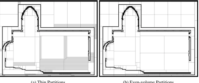
3.12 A comparison of the domain decomposition between a greedy splitting algorithm and the even-volume partitioning algorithm. . . 38
3.13 Error of an impulse response taken around 10 m away from the source on the Village scene using the MPARD method for a single band impulse at 225 Hz. . . 40
3.14 Comparison of impulse responses 10 m away from a 225 Hz source. . . 41
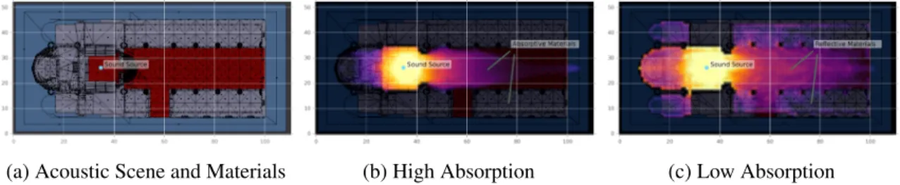
4.1 An example of how the materials in a building can affect the acoustic properties of
that building. . . 44
4.2 Our optimization pipeline, which computes the full derivative at the same time as it computes the pressure field. . . 51
4.3 Domain decomposition of a cathedral using the ARD method. . . 52
4.4 Dependencies of different subsystems of the ARD solver. . . 55
4.5 Geometry and material segmentation of the various benchmark scenes. . . 56
4.6 Comparison between different derivation methods: Automatic Differentiation and finite differences at10−5. . . 59
4.7 Impulse responses before and after optimization on each scene. . . 60
4.8 Cathedral field slices before and after optimization. . . 61
4.9 Twilight field slices before and after optimization. . . 61
4.10 Concert Hall field slices before and after optimization. . . 62
4.11 Overview of the scene geometry, source, and listener positions. . . 69
4.12 Experimental setup with material segments of each scene. . . 70
4.13 Convergence up to200iterations of the simulated annealing process in single-objective optimization. . . 72
4.14 Convergence of simulated annealing for adaptive initial temperature and early-cutoff. . . 72
4.15 The current energy per iteration of six different experiments optimizing for acoustic Strength (G) on the Concert Hall scene. . . 73
4.16 Impulse responses before and after individual optimization optimization. . . 74
4.17 Full-field top-down slices for the Cathedral scene showing the difference from the target metric before and after optimizing for various acoustic parameters. . . 75
4.18 Full-field top-down slices for the Concert Hall scene showing the difference from the target metric before and after optimizing for various acoustic parameters. . . 76
4.19 Full-field top-down slices for the Cathedral scene showing the difference from the target metric before and after multiobjective optimization. . . 78
4.20 Full-field top-down slices for the Concert Hall scene showing the difference from the target metric before and after multiobjective optimization. . . 79
4.21 Logarithmic plot of reverberation time for ARD compared to Sabine and Eyring. . . 80
4.23 Full-field plot showing the difference between the reverberation time at each grid
point using our discrete optimization technique and using Sabine’s equation. . . 80
5.1 The importance of diffraction (low frequency) effects in sound propagation. . . 84
5.2 Combining impulse responses for hybrid acoustic sound propagation. . . 86
5.3 The A, B, and C-weighting curves . . . 91
5.4 The optimization algorithm. . . 92
5.5 Clustering allows us to represent large areas of possible source locations by a single (virtual) source location. . . 95
5.6 THe benchmark scenes: the office scene, the warehouse scene, and the industrial scene. . . 98
5.7 The spectrograms of various sound sources that we used in our benchmarks and evaluated their noise effects. . . 99
5.8 The time spent during each iteration for the three benchmarks. . . 100
5.9 Noise field slice for the office scene calculated with ARD using the impulse response at every location. . . 102
5.10 Noise field slice for the warehouse scene calculated with ARD using the impulse response at every location. . . 102
5.11 Noise field slice for the industrial scene calculated with ARD using the impulse response at every location. . . 103
5.12 Change in the noise field for the office scene. . . 103
5.13 Change in the noise field for the warehouse scene. . . 104
5.14 Change in the noise field for the industrial scene. . . 104
5.15 Error comparison with a high resolution numerical simulation on the office scene. . . 105
5.16 Error comparison with a high resolution numerical simulation on the warehouse scene. . . 106
5.17 We highlight various components of our approach. . . 108
5.18 Diagram of the placements constraints used in the discretization of a portion of the Office scene. . . 109
5.19 Side-by-side comparison of the minimal and maximal locations for the receiver according to our optimization process. . . 112
5.20 Convergence plot of our optimization process in different environments. . . 112
CHAPTER 1: INTRODUCTION
Sound is ubiquitous in our lives and has a widely-varying effect on audibility, health, comfort, learning, and enjoyment. Therefore, the architectural design of theaters, hospitals, workplaces, schools, and concert halls take into account sound propagation, or the manner in which sound travels throughout an environment. For example, hospitals must be designed in a way to minimize the impact of environmental noise, since this noise can have a negative effect on health and recovery (Basner et al., 2014). The World Health Organization publishes guidelines for acceptable environmental noise levels (Birgitta et al., 1999) for hospitals.
Similarly, the quality of concert halls can be described by various acoustic metrics. These metrics measure the impact of the propagation environment on the sound that the audience hears. Auditoriums and lecture halls have similar requirements — it is important that audience members are able to hear the speaker clearly and understand them.
Furthermore, these design considerations are often incorporated early in the architectural design process. Changing the way in which sound propagates in an environment after it is built is difficult, and can sometimes amplify fundamental acoustic problems in the design (Egan, 1988). As such, many architects use mathematical or computer models to analyze the effects of sound propagation in their designs.
1.1 Models for Sound Propagation
Sound travels as a wave through an elastic medium, such as air, water, and solid objects such as materials commonly used in construction. Sound waves are longitudinal, and driven by the compression and rarefaction of the medium. In air, these waves change atmospheric pressure as they propagate: areas of compression contain the highest pressure, while areas of rarefaction reduce the pressure below normal atmospheric conditions. As such, sound from a simple pure tone travels through air in a sinusoidal manner, with the period being inversely proportional to the frequency of the sound source.
changes depending on varying temperature and humidity in air. However, in this discussion, we assume a homogeneous environment with a constant speed of sound, denoted asc= 343 m s−1.
Sound from a source travels directly in a path outwards from the source. When encountering obstacles, the sound maybe be reflected, where it continues at an equivalent angle off of a surface; diffused, where sound is scattered in a random manner from the surface; diffracted, or bent around an obstacles smaller than the wavelength of the sound; transmitted through an obstacle; or absorbed. Wave phenomena such as diffraction and scattering can have a significant effect on auralized sound (Torres et al., 2001a,b).
These propagation effects are governed by the time-domain wave equation in a homogeneous domain:
∂2
∂t2p(~x, t)−c
2∇2p(~x, t) =f(~x, t), (1.1)
where the pressure at timetand spatial position~xisp(~x, t), the constant speed of sound isc, ∇2 is the Laplacian, andf(~x, t)is a term for forcing sound pressure, used to represent a sound source or external boundary conditions on the domain.
An important concept in architectural acoustics is that of the room impulse response (IR). The impulse response is the output of an acoustic system when excited by an impulse source signal. Such a source signal can be defined by the Dirac functionδ(t−t0), which has an infinite value att0and a value of zero everywhere else. The spectrum of the Dirac function is thus given by a constant value for all frequencies. Given a Dirac source signal at~x1, wheret0is the starting time delay of the sound source, solving Equation 1.1 at a specific listener location location~x2over a sufficient period of time will yield the impulse responser(t) at that location.
The outputs0(t)of an acoustic system with respect to a source signals(t)can then be obtained by the convolution of the source signal with the impulse response originating from the same location (Kuttruff, 2016):
s0(t) =s(t)∗r(t) (1.2)
Additionally, the impulse response is useful for the evaluation of various acoustic metrics used in architectural acoustics. The impulse response function varies depending on the source and listener positions
~
Therefore, a fundamental aspect of evaluating a room or structure for the purposes of acoustic design is measuring or computing the impulse response. Computer models for evaluating the impulse response are particularly useful early in the design process when the structure is not actually built and the impulse response cannot be measured. However, Equation 1.1 is a partial differential equation (PDE) that has no closed form solution on arbitrary complex domains. As a result, many techniques have been developed for numerical approaches to solving these problems.
Typical techniques for solving sound propagation problems fall under two primary categories: geometric methods and wave-based methods. Geometric methods use the underlying assumption of sound waves being able to be represented by geometric primitives such as rays, beams, frustums, etc. (Funkhouser et al., 2003). Such techniques are usually compute performance-dependent logarithmically on the geometric complexity of the environment and the number of source and listener locations, but are efficient enough for real time applications. The drawback to geometric approaches is the limited ability of geometric representations of sound waves to capture all wave phenomena, including diffraction and scattering. There are geometric approaches for approximating scattering effects, but these techniques are often accurate only for low-order diffraction (Tsingos et al., 2001). Given the importance of scattering at lower frequencies, where obstacles are of similar size to the wavelength of propagated sound, geometric techniques are not sufficiently accurate to represent lower frequencies of sound propagation for the purpose of acoustic evaluation and design.
1.2 Acoustic Optimization
Multidisciplinary design optimization (MDO) is a wide ranging area of research in engineering and design. The primary focus of MDO techniques are to integrate various aspects of the design process, including structure, vibration, acoustics, and so on. It is commonly used in many areas including aerodynamic optimization of wings and entire aircraft, architectural features such as bridges and buildings, railway cares, microscopes, automobiles, turbines, and ships (Martins and Lambe, 2013). MDO applications intrinsically imply some sort of interface or constraint in a design process. For example, the structural design of a building may enforce constraints on what kind of acoustic materials may be used. This has an impact on the acoustic design of the building. We are particularly interested in how these techniques can be applied to acoustics and be used for improving the acoustics of a design while conforming to constraints in the design process.
The main purpose of acoustic design optimization is to change the shape, materials, topology, or source/listener positions in order to improve specific qualities of propagated sound. For example, shape optimization could include changing the dimensions of balconies in a concert hall to improve the distribution of acoustic energy in a scene, such as in (Robinson et al., 2014). Material optimization techniques attempt to change what materials are used in a design or to place acoustic absorbers to improve sound (Saksela et al., 2015). Topology optimization, such as the method proposed in D¨uhring et al. D¨uhring et al. (2008), involve generalized changes in the structure of a design, including placement of sound barriers, columns, walls, doorways, etc. The degree of freedom involved in topology optimization processes, however, makes this class of problems more challenging to solve. Finally source/listener position optimization problems typically involve the placement of speakers for sound field reproduction (SFR) applications or the design of home theater systems. These approaches typically select optimal placements for either sound sources or receivers (like a microphone or human listener).
Figure 1.1: Plots showing permissible noise exposure and the noise weighting curves commonly used in regulatory agencies such as OSHA (OSHA, 2008). Human beings can suffer health problems or hearing damage from instantaneous exposure to noise over 115 dB or noise over 90 dB over the course of an 8-hour workday. Noise levels are weighted according to various weighting curves, including the most commonly used A-weighting curve that is adjusted according to the human frequency response to sound.
sound propagation (Monks et al., 2000; Saksela et al., 2015; Bassuet et al., 2014) which are efficient, but lack accuracy at lower frequencies.
Some of the optimization applications where acoustic design is important include concert hall and theater design, noise minimization, and sound environment reproduction.
The problem of designing theaters and concert halls for appealing audience experience is as old as the ancient Roman architects (Pollio, 1914). Everything, from the material used in construction, the size of architectural features, the topology, and the placement of the performers or audience can affect the acoustics and audience experience. Modern work in this area includes work by Bassuet et al. (2014), Robinson et al. (2014), and Monks et al. (2000) in the area of concert hall design.
Figure 1.2: Side-by-side comparison of how speech intelligibility at the receiver location of an ASR device can change according to its location. Each datapoint on this plot corresponds to a user standing at that position and interacting with the ASR device. The STI metric used here is explored in more detail in Chapter 5.
Another recent field where noise has a detrimental effect is that of automatic speech recognition (ASR) algorithms (Rabiner and Juang, 1993). These algorithms translate spoken audio clips to text for a variety of applications including home automation systems, smart devices, electronic personal assistants, and so on. These techniques generally suffer under conditions of excessive noise and reverberation (Gillespie and Atlas, 2002). An open area of research is how these problems can be minimized through acoustic changes in the environment or placement of ASR devices. Figure 1.2 shows how simply relocating the receiver for an ASR device in a home can affect the quality of received sound.
Optimization procedures can also be used for the purpose of reproduction of sound environments. The placement of speakers for the purpose of sound field reproduction (SFR) in acoustic signal processing can be accomplished using acoustic optimization technique (Khalilian et al., 2015). It is also possible to use optimization techniques to match simulated and measured impulse responses for the purpose of discovering the acoustic material properties of various surfaces in the environment (Schissler et al., 2017).
1.3 Challenges
Figure 1.3: A top-down slice of the simulation domain of the ˇSibenik Cathedral. The overall size of the scene is 38×18×30 m, which comes out to around3.6x1012cells in an FDTD discretization. Using FDTD the compute costs of sound propagation on this scene for the full range of human hearing are around 150 exaflops.
scattering. Diffraction occurs when the size of an obstacle is similar to the wavelength (Egan, 1988); given
c= 343 m s−1, obstacles of a sizedmeters will produce diffraction effects at 343d Hz. Thus, a simple doorway a little over a meter wide is sufficient to diffract sound at around 350 Hz, which is well within the range of human speech and is similar in pitch to the mid-range of many orchestral instruments. Since geometric techniques do not accurately represent such phenomena, they can be inaccurate for architectural acoustic problems.
However, the aforementioned computational complexity of wave-based techniques make the problem of sound propagation using numerical methods a challenging prospect in many architectural scenes. Consider a large architectural scene, such as the Cathedral of St. James in ˇSibenik, Croatia (Figure 1.3). The simulation domain of this scene is almost 20 000 m3. Spatially discretizing this environment for a standard FDTD method yields a grid composed of around 3 trillion cells. The total compute cost for evaluating an impulse response for the cathedral at 20 kHz (the full range of human hearing) is around 150 exaflops. Assuming best-case peak compute, an NVIDIA Tesla K80 GPU would take 4 days to compute this sound propagation problem. Similarly, an Intel Xeon Phi would take 12 days to finish. This is in addition to a total memory use of 28 terabytes, which is too large for the memory capacity of existing general purpose computing accelerators.
wave phenomena are not being accurately captured. Particularly when diffraction effects can have a significant impact on the sound that human beings hear, geometric solvers are not sufficiently accurate for architectural approaches (Savioja, 2010a). However, despite this and because of the performance advantages to using geometric approaches, they are prevalent in real-time auralization and analysis.
The performance disparity between geometric and wave-based approaches is even more apparent in acoustic optimization applications. In most optimization applications, the acoustic field or impulse response must be computed in the evaluation of the objective function (for example, in Monks et al. (2000) ). Thus, optimization schemes with a large number of iterations (say, in the hundreds) is not tractable for most wave-based approaches on architectural environments and are often limited to smaller domains. Robinson et al. (2014), for example, use only a 2D approach in their concert hall shape optimization algorithm. However, in some optimization applications, it is possible to reduce the number of iterations and the number of solves required in evaluation of the objective functions. This approach can dramatically improve the performance of design optimization processes that use wave-based techniques.
A second element of difficulty that has implications on performance and accuracy is that many archi-tectural acoustic problems have complex domains — it is straightforward to evaluate the propagation of sound in a simple scene such as a rectangular room (in fact, analytic solutions of the wave equation are possible (Kuttruff, 2016)), but more complex domains do not have closed form solutions to the wave equation.
Additionally, it is often desirable to enforce constraints on any kind of acoustic optimization process. For example, to avoid some of the problems mentioned earlier with materials that may be acoustically desirable, but not structurally practical, it is important to be able to constrain materials so that only certain materials are selected by the optimization process. In other acoustic problems, such as microphone or speaker placement, it is often the case that microphones and speakers cannot arbitrarily be placed in the scene. For example, a speaker array may obstruct a particular audience view. This can limit the scope of some optimization approaches.
performance. Multiobjective optimization techniques can have difficulty converging, and thus can impact the number of iterations and number of evaluations of the objective function.
1.4 Thesis Statement
Large-scale distributed parallel wave-solvers and hybrid solvers can be used to accurately and efficiently
solve acoustic propagation and optimization problems for computer-aided design.
The primary goal of this dissertation is to develop novel techniques for accurate and efficient sound propagation and optimization in architectural acoustics applications. Our focus is on computer-aided design, where simulation and optimization methods can be used to model how sound propagates in architectural environments and how the acoustic characteristics of a structure can be improved before the structure is constructed. First, we explore how large distributed parallel techniques can be used in conjunction with low-dispersion wave solvers in order to efficiently compute sound pressure fields on large indoor and outdoor domains. Second, we analyze how wave-based techniques can be used in acoustic material optimization problems. Finally, we discuss the limitations of solely wave-based approaches and how geometric techniques can be used to augment wave-based solutions for higher frequency sounds in the context of optimization problems.
1.5 Main Contributions
Figure 1.4: Scalability of the MPARD technique from 1024 to 16384 cores on the 5 kHz cathedral scene. We obtain close-to-linear scaling in this result. The base speedup is 1024 on 1024 cores (assuming 1024 cores is 1024 times faster than one core) since the scene will not fit in memory on a lower number of cores.
1.5.1 Parallel Wave-Based Sound Propagation
The computational and memory cost of accurate wave-based techniques for high frequencies is often in-tractable for architectural acoustic applications. Recent advances in low dispersion techniques have improved numerical dispersion errors of finite difference and finite element type solvers (Guddati and Thirunavukkarasu, 2016; Davis, 1991; Hu et al., 1996; Savioja and Valimaki, 2000a). As such, minimized dispersion error can reduce the number of samples required per wavelength of the discretization, allowing greater computational efficiency. One such technique, Adaptive Rectangular Decomposition (ARD) (Raghuvanshi et al., 2009b) minimizes dispersion error through the use of analytic subdomains, thus requiring 2-3 samples per wave-length as opposed to 10 samples per wavewave-length that is common in many FDTD methods. However, the computational cost is still well within the exaflop range for large acoustic problems at high frequencies.
Therefore, we propose a novel parallel ARD algorithm, called MPARD. This technique is scalable on large supercomputing clusters, tested up to16000cores (see Figure 1.4). Using this technique, we are able to simulate acoustic sound propagation on large indoor and outdoor architectural scenes up to 10 kHz frequencies. This is far beyond the limitations of traditional methods, which generally remain in the 1 kHz to 2 kHz range. The main contributions of this algorithm are as follows:
• Hypergraph partitioning for load balancing and minimizing communication cost among cores • A preprocessing step for allocating work efficiently among cores
These components of the algorithm ensure a linearly scalable technique that has been tested up to16000 cores. Additionally, we have evaluated the technique on various indoor and outdoor CAD models. Using this technique, we can efficiently and accurately solve acoustic propagation problems for high frequencies for the purpose of evaluating an acoustic design.
1.5.2 Wave-Based Techniques for Acoustic Material Optimization
A standing problem in acoustic design is that of selecting the correct materials for construction in order to yield the desired sound. Buildings such as concert halls and auditoriums often have certain desirable acoustic characteristics that can be measured using the impulse response produced by sound propagating.
We present two novel techniques for optimizing the acoustic materials used in the design of structures such as concert halls and auditoriums. In the first method, we use a continuous gradient-based optimization scheme for minimizing the distance of various acoustic metrics from the goal metrics. In the second method, we use a Pareto-optimal simulated annealing minimization technique for optimizing materials under discrete constraints. Overall, our contributions can be summarized as follows:
• Multiobjective optimization methods for determining acoustic materials that yield the desired acoustic properties in a CAD model
• Efficient evaluation of acoustic metrics using impulse responses computed by the ARD wave-based technique
• Automatic differentiation techniques for computing the analytical gradient, enabling faster convergence in continuous optimization
• A Pareto-optimal simulated annealing technique for discrete multiobjective optimization • Constraint-based optimization using acoustic material libraries
1.5.3 Hybrid Techniques for Acoustic Optimization
Previous wave-based optimization techniques are limited to lower frequencies, less than 500 Hz. With explicit time domain methods, the time step of the method is governed by the Courant-Friedrichs-Lewy condition (CFL). At higher acoustic frequencies, the time step becomes smaller, but the total time range of the simulation must remain the same for a scene. Therefore a large part of the computational cost of explicit time domain methods is due to the increase in the total number of simulation steps. This is not as straightforward to parallelize as the spatial domain and thus becomes a much larger factor in the performance of iterative optimization methods where the objective function may need be evaluated hundreds of times of the course of optimization.
To address these problems, we introduce an optimization technique using hybrid acoustic simulation. In hybrid propagation, we use expensive wave-based techniques for the lower simulation frequencies, where accurate solutions to the wave equation are necessary for representing effects such as diffraction and scattering that are more noticeable. Then, higher frequencies are simulated using geometric methods. At these frequencies, wave effects are less prevalent and wave-based methods are more expensive. We present two applications for this technique. The first application technique uses this hybrid approach in order to place noise emitters in an environment such that noise reaching specific listener regions is minimized. Our second application aims to improve the effectiveness of automatic speech recognition (ASR) hardware by placing the speech receiver in an environment where speech intelligibility is maximized. Our contributions include:
• A hybrid acoustic solver for improved efficiency while retaining the accuracy of solely wave-based approaches
• Sound source clustering for reducing the optimization search space
• Impulse response caching for reducing the number of solves required for evaluating the objective function • Adaptive start and end criteria for simulated annealing, reducing the number of optimization iterations
1.6 Organization
The rest of this dissertation is organized as follows:
Chapter 2 provides some of the mathematical background of the techniques used in the dissertation in addition to providing a survey of prior work in the topics covered.
Chapter 3 introduces parallel sound propagation with ARD and how it can be extended to compute clusters with tens of thousands of available cores.
Chapter 4 presents acoustic material optimization techniques using wave-based sound simulation for evalu-ating a variety of acoustic metrics.
Chapter 5 describes a frequency-partitioned hybrid sound propagation technique that is used for various optimization applications, including noise minimization and the maximization of speech intelligibility. Chapter 6 Concludes the dissertation, along with thoughts about limitations and future challenges in the
CHAPTER 2: BACKGROUND
This chapter provides an overview of some of the previous work in sound propagation research, along with work done in optimization and noise reduction. Background on the Adaptive Rectangular Decomposition method (ARD) that is central to many of the algorithms presented in this dissertation is also included.
2.1 Sound Propagation
Methods for solving the acoustic wave equation (Equation 1.1) are generally separated into two main categories: the geometric methods and the wave based methods.
2.1.1 Geometric Methods
Geometric methods generally model of sound propagating in the form of a ray or other geometric primitive, and work on the assumption that the wavelength of modeled sound is much smaller than the size of obstacles in the environment (Funkhouser et al., 2003).
Geometric methods tend to fall under the category of image source methods, ray tracing techniques, and beam tracing or frustum tracing approaches. Image source methods mainly consider specular paths of sound, i.e. sound that travels in a mirror-like manner when reflecting off an obstacle. They model sound by mirroring audio sources over polygonal surfaces in the environment. Image source methods were introduced by Allen and Berkley Allen and Berkley (1979). Additional approaches include a generalization to arbitrary-sided polyhedra (Borish, 1984). Schissler et al. Schissler and Manocha (2011) introduce a listener image method, where this technique is used to cache propagation paths in conjunction with backwards ray-tracing.
techniques for simulated diffraction and scattering effects include (Tsingos et al., 2001; Embrechts et al., 2001; Tsingos et al., 2007; Schissler et al., 2014a).
Beam tracing methods include intersections between geometry and pyramidal sets of rays. These approaches include beam tracing for interactive environments (Funkhouser et al., 1998), hybrid beam tracing and image source methods (Monks et al., 1996), and frustum tracing (Chandak et al., 2008).
2.1.2 Wave-Based Sound Propagation
Wave-based approaches, on the other hand, numerically solve the wave equation (1.1). These approaches encompass implicit and explicit time-domain algorithms. Wave-based approaches are generally limited to lower frequencies, as higher frequencies require dramatically more compute power and memory (compute costs asymptotically increase asO f4).
Finite-element techniques use a subdivision into linear elements for solving the Helmholtz equa-tion, and ensure convergence with either the collocation method or Galerkin method for global conver-gence (Funkhouser et al., 2003). FEM techniques include works by Nefske et al. Nefske et al. (1982) and Craggs Craggs (1972). An overview of these approaches can be found in Thompson Thompson (2006). Boundary-element methods work in a similar manner, and include approaches for solving radiation and scat-tering problems (Chen et al., 2010). An overview of boundary element methods can be found in (Ciskowski and Brebbia, 1991).
2.2 Adaptive Rectangular Decomposition
For the techniques put forth in this dissertation, we primarily use the Adaptive Rectangular Decomposition (ARD) solver (Raghuvanshi et al., 2009b; Mehra et al., 2012; Morales et al., 2015a), including mathematical details that are relevant to this thesis.
2.2.1 Pressure Field Computation
Consider a cuboidal domain in three dimensions of size(lx, ly, lz)with perfectly reflecting walls. The acoustic wave equation on this domain has an analytical solution represented as:
p(x, y, z, t) = X i=(ix,iy,iz)
mi(t)Φi(x, y, z), (2.1)
wheremi are the time-varying mode coefficients and Φi are the eigen functions of the Laplacian for the cuboidal domain, given by:
Φi(x, y, z) =cos
πix lx x cos πiy ly y cos πiz lz z . (2.2)
We limit the modes computed to the Nyquist rate of the maximum simulation frequency.
In order to compute the pressure, we need to compute the mode coefficients. Reinterpreting equation (2.1) in the discrete setting, the discrete pressureP(X, t)corresponds to an inverse Discrete Cosine Transform (iDCT) of the mode coefficientsMi(t):
P(X, t) =iDCT(Mi(t)). (2.3)
Substituting the above equation in Equation 1.1 and applying a DCT operation on both sides, we get
∂2
∂t2Mi+c 2k
i2Mi =DCT(F(X, t)), (2.4)
whereki2 =π2
ix2
lx2 + iy2
ly2 + iz2
lz2
the mode coefficients:
Min+1 = 2Mincos(ωi∆t)−Min−1+ 2
∼ Fn
ω2 i
(1−cos(ωi∆t)), (2.5)
where ∼
F =DCT(F(X, t)). This update rule can be used to generate the mode-coefficients (and thereby pressure) for the next time-step. This gives us a method to compute the analytical solution of the wave equation for a cuboidal domain. Next, we describe how these solutions are used to solve the wave equation over the entire scene.
2.2.2 Interface Handling
In order to ensure correct sound propagation across the boundaries of these subdomains, we use a (2,6) finite difference stencil to patch two subdomains together. A 6th order scheme was chosen because has been experimentally determined (Mehra et al., 2012) to produce reflection errors at 40 dB below the incident sound field. We derive the stencil as follows.
First, we examine the projection along an axis of two neighboring axis-aligned cuboids. Our local solution inside the cuboids assumes a reflective boundary condition, ∂x∂p
x=0 = 0. Looking at the rightmost
cuboidal partition, the solution can be represented by the discrete differential operator,∇2
local, that satisfies the boundary solutions. Referring back to the wave equation, we have the global solution:
∂2p
∂t2 −c 2∇2
globalp=f(X, t).
Using the local solution of the wave equation inside the cuboid (∇2
local), we derive:
∂2p ∂t2 −c
2∇2
localp=f(X, t) +fI(X, t),
wherefI(X, t)is the forcing term that needs to be contributed by the interface to derive the global solution. Therefore, we need to solve for this term, using our two previous identities:
fI(X, t) =c2 ∇2global− ∇2local
While the exact solution to this is computationally expensive, we can approximate the solution using a 6th order finite difference stencil, with spatial step sizeh:
fI(xj) = −1
X
i=j−3
p(xi)s[j−i]−
2−j
X
i=0
p(xi)s[i+j+ 1], (2.7)
wherej ∈[0,1,2],fI(xj) = 0forj >2, ands[−3. . .3] = 180h1 2{2,−27,270,−490,270,−27,2}.
Additionally, interfaces between subdomains that cover homogeneous air regions and subdomains that are solid are modeled by this method. The forcing terms for an air-wall interface are computed as follows:
fI(xj) = −1
X
i=j−3
p(xi)s[j−i]α− 2−j
X
i=0
p(xi)s[i+j+ 1]α, (2.8)
whereαis a material absorption value.
The absorption valueαis used to model absorption at air-wall boundaries. If this value is zero, then the FDTD stencil is not taken into effect and the wall is regarded as perfectly reflective. On the other hand, if the value is one, the FDTD is taken into full effect and the wave is propagated into the PML partition where it is absorbed. Similarly, values used between zero and one result in partial reflectance.
A limitation of this approach is that only a single absorption value is used that does not take into account the dependence on the frequency. For more realistic materials, it is necessary to run the simulator for multiple frequency bands, i.e. multiple bands in the human hearing range 20 Hz to 20 000 Hz, though in practice current solvers are limited to a few thousand kilohertz.
2.2.3 ARD computational pipeline
The ARD technique has two main stages: PreprocessingandSimulation. During the preprocessing stage, the input scene is voxelized into grid cells. The spatial discretization of the gridh is determined by the maximum simulation frequencyνmax determined by the relationh = c/(νmaxs), wheresis the number of samples per wavelength (=2.66 for ARD) andcis the speed of sound (343m/secat standard temperature and pressure). The next step is the computation of adaptive rectangular decomposition, which groups the grid cells into rectangular (cuboidal) domains. These generate the partitions, also known asair
partitions. Pressure-absorbing layers are created at the boundary by generating Perfectly-Matched-Layer
in the scene. Artificial interfaces are created between the air-air and the air-PML partitions to propagate pressure between partitions and combine the local pressure fields of the partitions into the global pressure field.
During the simulation stage, the global acoustic field is computed in a time-marching scheme as follows (see Figure 3.2 (top row)):
1) Local update
For all air partitions
(a) Compute the DCT to transform forceF to ∼ F. (b) Update mode coefficientsMiusing update rule. (c) TransformMito pressureP using iDCT.
For all PML partitions
Update the pressure field of the PML absorbing layer. 2) Interface handling
For all interfaces
(a) Compute the forcing termF within each partition. 3) Global update
Update the global pressure field.
The first stage solves the wave equation in each rectangular region by taking the Discrete Cosine Transform (DCT) of the pressure field, updating the mode coefficients using the update rule, and then transforming the mode coefficients back into the pressure field using inverse Discrete Cosine Transform (iDCT). Both the DCT and iDCT are implemented using fast Fast Fourier Transforms (FFT) libraries. Overall, this step involves two FFT evaluations and a stencil evaluation corresponding to the update rule. The pressure fields in the PML-absorbing layer partitions are also updated in this step.
The second stage uses a finite difference stencil to propagate the pressure field between partitions. This involves a time-domain stencil evaluation for each grid cell on the boundary.
CHAPTER 3: A Massively Parallel Solver for Large Compute Clusters
The main challenge is that the computational cost of computing the sound propagation in the environment scales with the 4th power of frequency and linearly with the volume of the scene, while memory use scales with the 3rd power of frequency and linearly with the scene volume. Since the human aural range scales from 20 Hz to 20 kHz, large scenes such as a cathedral (10 000 m3to 15 000 m3) would require tens of Exaflops of computation and tens of terabytes of memory to compute using prior wave-based solvers. This makes high frequency acoustic wave simulation one of the more challenging problems in scientific computation (Engquist and Runborg, 2003).
Recently, there has been a lot of emphasis on reducing the computational cost of wave-based methods. These techniques, calledlow dispersion techniquesuse coarser computational meshes or decompositions in order to evaluate the wave equation. One example of a low dispersion algorithm is the Adaptive Rectan-gular Decomposition method (ARD) (Raghuvanshi et al., 2009b; Mehra et al., 2012), a solver for the 3D acoustic wave equation in homogeneous media. ARD is a domain decomposition method that subdivides the computational domain into rectangular regions. One of the main advantages of ARD is the greatly reduced computational and memory requirements over more traditional methods like FDTD (Mehra et al., 2012).
Previously, ARD has been used to perform acoustic simulations on small indoor and outdoor scenes for a maximum frequency of 1 kHz to 2 kHz using only a few gigabytes of memory on a high-end desktop machine. However, performing accurate acoustic simulation for large acoustic spaces up to the full auditory range of human hearing still requires terabytes of memory. Therefore, there is a need to develop efficient parallel algorithms, scalable on distributed memory clusters, to perform these large-scale acoustic simulations. In this chapter, we discuss our algorithms for parallelizing ARD. This work was originally published in (Morales et al., 2015a) and (Morales et al., 2017).
Scaling to this number of CPU cores with such a large domain introduces many challenges, including communication cost, numerical stability, and reducing redundant computations. MPARD addresses all of these in a novel method that is comprised of:
• An efficient asynchronous communication technique for overlapping communication between cores with computation
• A hypergraph partitioning approach for load balance and communication reduction among multiple nodes
• A subdomain splitting algorithm to maintain the numerical accuracy of our wave-based simulator while ensuring subdomain computations are load balanced
MPARD is capable of computing the acoustic propagation in large indoor scenes (20 000 m3) up to at least 10 kHz at around 80 s per time step on1024cores. The algorithm has been tested to and scales up to at least16000cores, where each time step of a 5 kHz scene takes around 0.2 s. We have analyzed many aspects of our parallel algorithm including the scalability over tens of thousands of cores, the time spent in different computation stages, communication overhead, and numerical errors. To the best of our knowledge, this is one of the first wave-based solver that can handle such large domains and high frequencies.
3.1 Previous work
There has been considerable research in the area of wave-based acoustic solvers, including the field of parallel solvers, domain decomposition approaches, and low-dispersion acoustic solvers. In this section, we provide a brief overview of some of these approaches.
3.1.1 Parallel wave-based solvers
Additionally, there are several parallel methods developed for specific applications of the wave equa-tion. PetClaw (Alghamdi et al., 2011) is a scalable distributed solver for time-dependent non-linear wave propagation. Other methods include distributed finite difference frequency-domain solvers for visco-acoustic wave propagation (Operto et al., 2007), discontinuous Galerkin solvers for heterogeneous electromagnetic and aeroacoustic wave propagation (Bernacki et al., 2006), scalable simulation of elastic wave propagation in heterogeneous media (Bao et al., 1998), etc.
3.1.2 Domain decomposition
MPARD, like ARD, is a domain decomposition method. Domain decomposition approaches subdivide the computational domain into smaller domains that can be solved locally. The solver uses these local solutions to compute a global solution of the scientific problem. Many of these approaches are designed for coarse grain parallelization where each subdomain or a set of subdomains is computed locally on a core or a node on a large cluster.
Domain decomposition approaches tend to fall into two categories: overlapping subdomainand
non-overlapping subdomainmethods (Chan and Widlund, 1994).
Existing domain decomposition approaches in computational acoustics include parallel multigrid solvers for 3D underwater acoustics (Saied and Holst, 1991), pseudospectral acoustic solvers (Hornikx et al., 2016; Zeng et al., 2004), and the non-overlapping subdomain ARD approach (Raghuvanshi et al., 2009b). Additional non-overlapping approaches include Trefftz methods that can be decomposed for parallelization (Pluymers et al., 2007) and line source decomposition methods for ESM (equivalent source method) techniques (Hornikx and Forss´en, 2007).
3.1.3 Low dispersion acoustic solvers
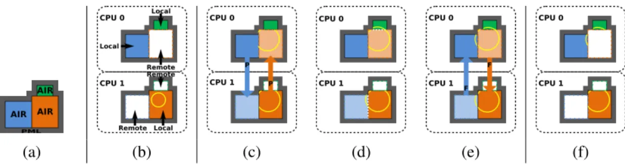
(a) (b) (c) (d) (e) (f)
Figure 3.1: The parallel ARD pipeline. The initial partitioning and voxelization is the input into the simulation (a). Next, the local partition update occurs, evaluating the exact solution for an individual partition rectangle (b). In order to calculate interfaces, we need to transfer the pressure terms from the spanned partitions to the core that is evaluating the interface (c). The interface is then evaluated (d) and the forcing terms transferred back (e). Finally, global update occurs as the forcing terms are used to compute the global pressure field (f).
Our approach is primarily based on the ARD method (Raghuvanshi et al., 2009b) which partitions the computational domain into rectangular regions. It utilizes the property that the wave equation has a closed form solution in a homogeneous rectangular domain. Therefore, the only numerical error originates from the interfaces between these rectangular regions, allowing a much coarser grid size.
3.2 Parallel ARD
Table 3.1 summarizes the problem size limitations of previous ARD algorithms (see Chapter 2), including parallel ARD. Previous algorithms have been limited to problem sizes under 1 kHz to 2 kHz on large architectural scenes. The MPARD algorithm, on the other hand, is capable of operating on frequencies an order of magnitude greater than previous ARD methods. However, all algorithms are based on the same fundamental principles.
Solver Num. Cores Maximum Frequency on Cathedral
ARD (Raghuvanshi et al., 2009b) 1 1000 Hz to 2000 Hz
GPUARD (Mehra et al., 2012) 480 CUDA cores 1650 Hz
MPARD 16384 10 000 Hz
3.2.1 Partition and Interface Ownership
This first step of parallelization involves distributing the problem domain onto the cores of the cluster. In the case of ARD, the different domains include air partitions, PML partitions, and the interfaces.
Air and PML partitions: The ARD solver can be parallelized because the partition updates for both the air and the PML partitions are independent at each time step: each partition update is a localized computation that does not depend on the data associated with other partitions. As a result, partitions can be distributed onto separate cores of the cluster and the partition update step is evaluated in parallel at each time step without needing any communication or synchronization. In other words, each core exclusively handles a set of partitions. Theselocal partitionscompute the full pressure field in memory. The rest of the partitions are marked asremote partitionsfor this core and are evaluated by other cores of the cluster. Only metadata (size, location, etc.) for remote partitions needs to be stored on the current core, using only a small amount of memory (see Figure 3.1 (b)).
Interfaces: Interfaces, like partitions, retain the concept of ownership. One of the two cores that owns the partition of an interface, takes ownership of that interface, and is responsible for performing the computations with respect to that interface. Unlike the partition update, the interface handling step has a data dependency with respect to other cores. Before the interface handling computation is performed, pressure data needs to be transferred from the dependent cores to the owner (Figure 3.1 (c)). In the next step, the pressure data is used, along with the source position, to compute the forcing terms (Figure 3.1 (d)). Once the interface handling step is completed, the interface-owning core must send the results of the force computation back to the dependent cores (Figure 3.1 (e)). The global pressure field is updated (Figure 3.1 (f)) and used at the next time step.
3.2.2 Parallel Algorithm
Local Update: This step updates the pressure field in the air and PML partitions for each core independently, similarly to the basic ARD algorithm (see Chapter 2 for details). However, only partitions owned on a core are evaluated. Therefore, each core computes the local step in parallel with other cores.
Pressure field transfer: After an air partition is updated, the resulting pressure data is sent to all interfaces that are dependent upon this data. The pressure data is transferred to the destination core asynchronously as soon as it becomes available. Partitions are evaluated in order from partitions with the most neighbors to those with the least neighbors; this ensures that dependent interfaces are not starved of pressure data. Interface handling: This stage uses the pressure transferred in the previous stage to compute forcing terms for the partitions. Before the interface can be evaluated, it needs data from all of its dependent partitions. Since partitions are evaluated in order of the number of dependent interfaces, data starvation is minimized. Force transfer: After an interface is computed, the owner needs to transfer the forcing terms asynchronously back to the dependent cores. A core receiving forcing terms can then use them as soon as the message is received.
Global update: Each core updates the pressure field using the forcing terms received from the interface operators.
Barrier synchronization: A barrier is needed at the end of each time step to ensure that the correct pressure and forcing values have been computed. This is necessary before local update is performed for the next time step.
3.2.3 Efficient Load Balancing
For each time step, the computation time is proportional to the time required to compute all of the partitions. This implies that a core with larger partitions or more partitions than another core would take longer to finish its computations; this would lead to load imbalance in the system, causing the other cores of the cluster to wait at the synchronization barrier instead of doing useful work. Load imbalance of this kind results in suboptimal performance.
partitions and large number of small partitions. In a typical scene (e.g. the Cathedral benchmark), the load imbalance results in poor performance.
A naive load balancing scheme would reduce the size of each partition to exactly one voxel, but this would negate the advantage of the rectangular decomposition scheme’s use of analytical solutions; furthermore, additional interfaces introduced during the process at partition boundaries would reduce the overall accuracy of the simulator (Raghuvanshi et al., 2009b). The problem of finding the optimal decomposition scheme to generate perfect load balanced partitions while minimizing the total interface area is non-trivial. This problem is known in computational geometry asink minimization(Keil, 2000). While the problem can be solved for a rectangular decomposition in two dimensions in polynomial time, the three-dimensional case is NP-complete (Dielissen and Kaldewaij, 1991). As a result, we approach the problem using a top-down approximate technique that bounds the sizes of partitions and subdivides large ones yet avoids increasing the interface area significantly. This is different from a bottom-up approach that would coalesce smaller partitions into larger ones.
Each rectangular region that has a volume greater than some volume thresholdQis subdivided by the new algorithm.Qis determined by the equation
Q= V
pf, (3.1)
whereV is the total air volume of the scene in spatial discretization units,pis the number of cores the solver is to be run on, andf is the balance factor. It is usually the case thatf = 1, although this can be changed to a higher value if smaller rectangles are desired. However, in general, smaller values ofQincrease the overall interface error of the solver since it increases the total interface area.
3.3 Scaling to Large Clusters
3.3.1 Communication efficiency
Each interface in the scene covers two or more subdomains (for example, if the subdomains on either side are especially thin, the 6th order stencil may cover more than two). When subdomains on an interface are owned by different cores, the pressure terms required by the interface and the forcing terms generated by the interface need to be communicated.
MPARD uses asynchronous communication calls to avoid blocking while sending messages. When a core completes an operation (either a subdomain update or an interface update), it can send off a message to the cores that require the computed results. The sending core does not have to wait for the message to be received and can continue working on the next computation. When receiving data, a core can place the message on an internal queue until it needs the data for that operation. As a particular core finishes working on a subdomain, it sends off an asynchronous communication message to cores that require the pressure field of that subdomain for interface computation. As the message is being sent, that particular core begins to process the next subdomain, sending off a message upon completion. At the same time the receiving core is working on its own subdomains. The incoming message is stored on an internal queue for use when needed. Another important thing to note is that in general ARD’s communication cost of evaluating all the interfaces is proportional to the surface area of the rectangular region while the cost of evaluating each subdomain is proportional to the volume of the subdomain. This implies a roughO(n2)running time for interface evaluation (wherenis the length of one side of the scene) while local update has anO(n3)running time. This means that as the size of the scene or the simulation frequency increases, the computation cost of local update dominates over the communication cost of transferring pressure and forcing values for interface evaluation. On the other hand the finer grid size of larger complex scenes can introduce many more interfaces which causes an increase in the cost of communication.
In order to evaluate these interfaces, communication is only required when resolving the interface between two or more subdomains that lie on different cores. As a result, minimizing the number of these interactions can greatly reduce the total amount of communicated data.
(a) (b) (c) (d)
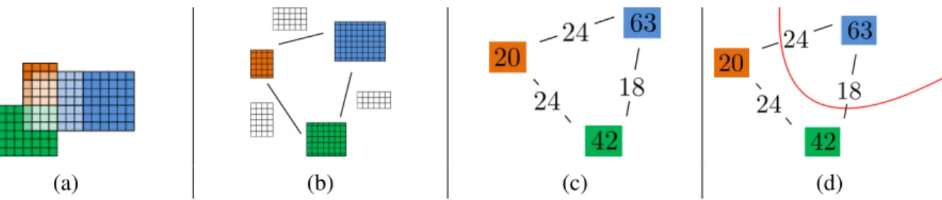
Figure 3.2: The relationship between computational elements of MPARD (rectangular subdomains and interfaces) and the hypergraph structure. (a) shows an example scene of three subdomains with three interfaces (shown in grey). The organization of the resulting hypergraph is shown in (b), while (c) shows the hypergraph with the node weights determined by the sizes of the rectangles and the hyperedge weights determined by the size of the interfaces. Subfigure (d) shows an example partitioning of the simple graph, taking into account both the computation cost of each node and the cost of each interface.
This problem can be reworded as a hypergraph partitioning problem. Our hypergraph can be represented as the pairH= (X, E)whereX, the nodes of the hypergraph are the rectangular regions of our decomposi-tion, while the hyperedgesErepresent the interfaces between the rectangular regions. Hyperedges are used rather than regular edges because an interface can actually cover more than two subdomains.
The goal of the hypergraph partitioning algorithm is to divide the hypergraph intokregions such that the cost function of the hyperedges spanning the regions is minimized (C¸ ataly¨urek and Aykanat, 2011). In ARD, the partitioning algorithm can be run to divide our computational elements (interfaces and rectangles) intok
regions, wherekis the number of processors used in the simulation. As a result, the interface cost between cores is minimized.
Additionally, because the hypergraph partitioning algorithm attempts to generatekregions of equal cost, the heuristic serves as a way of load balancing the assignment of work to cores. The cost of evaluating a rectangular region is linearly related to the volume of the region. Therefore, we can input the volume of each rectangular subdomain as the weight parameter for a node in the hypergraph.
core roughly equal volume, which is linearly related to computation time. We use the following connectivity metric to determine the cost of communication across boundaries:
C(Π) = X n∈NE
wn(λn−1), (3.2)
whereC(Π)is the cost of a particular partitioningΠ,NE is the set of cut hyperedges, wnis the weight of hyperedgen, andλnis the connectivity of the hyperedge. This metric is particularly useful because it prioritizes hyperedges that connect many vertices and is such directly proportional to the computation cost.
3.3.2 Load balancing and numerical stability
The splitting algorithm for load balancing introduced in earlier minimizes the number of extra interfaces created by splitting in some cases. The larger of the resulting subdomains is exactly below the maximum volume threshold of the splitting algorithm.
However, on a cluster with a higher number of cores and where the volume threshold can be relatively small, this splitting algorithm can introduce a series of very small and thin rectangles. Small and thin rectangles can create numerical instability during interface resolution. These errors are caused by the interaction between multiple overlapping interfaces.
Care must be taken to address these numerical problems. In this particular case, it is more advantageous to have wider rectangular subdomains that may introduce more interface area rather than degenerate rectangles which can result in numerical issues. A revised approach favors well-formed subdomains that are more cuboidal in shape rather than long and thin rectangles by choosing a subdivision on the minimal axis.
3.3.3 Interface and PML computation
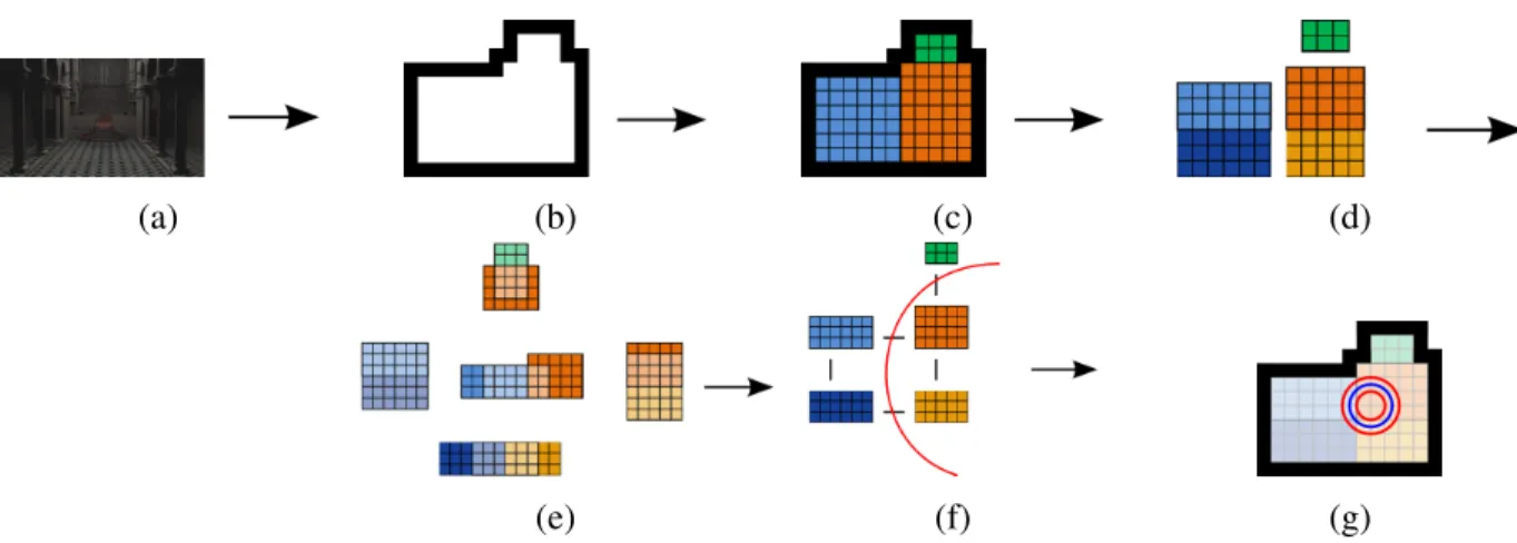
(a) (b) (c) (d)
(e) (f) (g)
Figure 3.3: The MPARD pipeline. The input geometry (a) is voxelized in the first step (b). The rectangular decomposition step divides the domain into multiple non-overlapping subdomains (c). The splitting step then splits these subdomains when they are greater than the volume thresholdQ(d). These partitions are then processed by the interface initialization stage which computes interface metadata (e). The final preprocessing stage allocates subdomains to nodes using the hypergraph partitioning (f). Finally, the simulation is run (g).
In order to reduce the running time of the simulation, MPARD introduces a new preprocessing step in which the interfaces can be initialized offline. This preprocessing step occurs after any splitting and load balancing, after the decomposition for the scene is final.
Additionally, this extra preprocessing step allows for further memory optimization in MPARD. With the kind of global metadata computed in the preprocessing, each core only needs to load the exact interfaces and PML regions it needs for its computations.
3.3.4 MPARD Pipeline
3.3.4.1 Voxelization
The voxelization stage takes in a triangle mesh representing the environment in which we want to compute the sound propagation. Because MPARD targets large and high frequency scenes that may consume a large amount of memory, we use a CPU method for voxelization. We implement anaccurateandminimal
method (meaning voxels should fully cover the geometry but not more than necessary) as introduced by Huang et al. (Huang et al., 1998).
The spatial discretization for the voxelization is determined by the minimum simulated wavelength and the required number of spatial samples per wavelength, which is typically between 2 and 4 (Raghuvanshi et al., 2009b). Therefore, the voxelization only needs to be run once per desired maximum frequency.
3.3.4.2 Decomposition
The decomposition stage then reads the voxel field and determines the location of the different cuboidal subdomains. The process is a greedy approach, attempting to expand each rectangular subdomain into as large a volume as possible under the constraints of the wall voxels.
At very high frequencies, such as 10 kHz, this process can take several days to complete but only needs to run once for a given voxel input.
3.3.4.3 Core allocation and subdomain splitting
The next stage of the preprocessing is the core allocation and subdomain splitting stage. In addition to a decomposition computed in the previous stage, this step also requires the number of cores the solver will run on. This stage uses the input values to compute a hypergraph partitioning for the decomposition in addition to splitting any rectangular regions that have volumes greater than the volume thresholdQ.
The core allocation stage then determines the assignment of subdomains to cores by using the hypergraph partitioning assignment or alternatively a simple bin-packing algorithm. This load balancing step ensures that each core has a roughly equal amount of work to complete during the acoustic simulation.
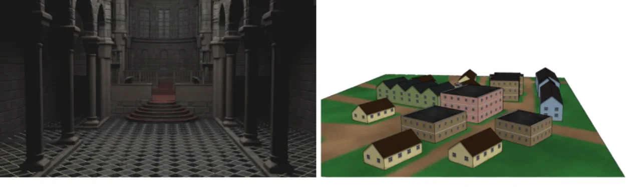
Scene Name Volume Frequency Number of Triangles Cathedral 19 177 m3 5 kHz, 10 kHz 55415
Village 362 987 m3 1.5 kHz 358
Table 3.2: Dimensions and complexity of the scenes used in our experiments. The input triangle mesh is voxelized according to the simulation frequency.
3.3.4.4 Interface and PML preprocessing
The final stage of preprocessing computes interfaces and creates PML regions from wall voxels. This stage takes as input a modified decomposition from the core allocation and splitting stage in addition to a refinement parameterrthat can be used to subdivide voxels in the final acoustic simulation. This allows us to run atrtimes the frequency the decomposition was run at. However, this is at the expense of some accuracy where high frequency geometric features of the scene that may affect sound propagation cannot be accurately represented.
One additional caveat of the interface and PML preprocessing file is file read performance in the simulator. The interface file can be several GBs in size, and thousands of CPU cores reading the file can cause a bottleneck. As a solution, we use the file striping feature of the Lustre file system (Schwan, 2003) to increase file read performance over all cores.
The interface and PML initialization stage only needs to be run once for each core configuration.
3.4 Results and analysis
Our method was tested on two computing clusters: the large-scale Blue Waters supercomputer (Bode et al., 2012) at the University of Illinois and the UNC KillDevil cluster. Blue Waters is one of the world’s leading compute clusters, with362240XE Bulldoze CPU cores and 1.382 PB of memory. The KillDevil cluster has9600CPU cores and 41 TB of memory.