Low Field MRI Using Halbach Ferromagnet Arrays

(1)

Low Field MRI using Halbach

Ferromagnet Arrays

THESIS

submitted in partial fulfillment of the requirements for the degree of

BACHELOR OF SCIENCE

in

PHYSICS

Author : K. van Deelen

Student ID : s1282220

Supervisor : A.G. Webb

(2)

(3)

Low Field MRI using Halbach

Ferromagnet Arrays

K. van Deelen

Huygens-Kamerlingh Onnes Laboratory, Leiden University P.O. Box 9500, 2300 RA Leiden, The Netherlands

July 20, 2017

Abstract

Since its discovery MRI quickly became an essential medical tool to help doctors make prognoses, as it allows one to look inside the

body without using invasive techniques like CAT-scans or surgery. However, MRI’s are very expensive: around one million

US dollars per Tesla of magnetic field, and require advanced facilities in order to operate (e.g. liquid helium), and thus are not accessible all over the world. This research explores developing a simpler and less expensive MRI, using ferromagnets in a Halbach

(4)

(5)

Chapter

1

Introduction

Ever since its discovery in 1971 by Paul C. Lauterbur [1], Magnetic Reso-nance Imaging (MRI) quickly became an essential tool in modern hospitals in the western world. With it, doctors can make prognoses without using invasive techniques, like CAT-scans or surgery, while still being able to make sharp images due to the high contrast in soft and hard tissue. These images tend to have high resolution, due to the high magnetic fields gen-erated by the superconducting coils in the MRI.

Unfortunately, high field MRI is very expensive, costing around one million US dollars per Tesla of magnetic field, and needs advanced facili-ties in order to work, e.g. liquid helium cooling and an separately shielded location in the hospital, because of the high stray magnetic field around the scanner. These requirements prevent this technique from being acces-sible in some parts of the world, like Asia and Africa [2]. Considering that every hospital should have access to MRI, but sometimes lack the funds or tools required to operate one, it is important to explore less expensive and more compact methods in order to make MRI more accessible around the world.

(6)

6 Introduction

In this research, the focus will be on making a low field MRI using fer-romagnets in a Halbach array to make images of a child’s head with high enough resolution to prognose Hydrocephalus, which is a common afflic-tion in 3rd world countries and needs cranial imaging techniques such as ultrasonography, CT or MRI in order to be diagnosed [10, 11]. The resolution of the image depends on the strength and homogeneity of the magnetic field in the to be scanned volume. A higher strength magnetic field results in more signal and thus higher signal to noise ratio which leads to a higher resolution. In a Halbach ring the strength of the mag-netic field increases with the number of magnets used and decreases with the radius of the ring. MRI depends on the assumption that the magnetic field in the measurable area is (roughly) the same. This requirement trans-lates in the form of the homogeneity of the magnetic field. Ultimately we have to make a trade-off between image resolution, image volume, price and weight of the MRI system. Multiple designs will be simulated and evaluated using commercial physics simulation software, COMSOL Mul-tiphysics v5.2 [12].

Once we have created a strong and homogeneous enough field, we still need to transmit and receive Radio Frequency (RF) signal in order to process the magnetic resonance data into an image. We will look into a method using a single RF coil as both a transmitter and receiver. The receiver and transmitter should be separated, as the strong transmitted RF pulse can damage the receiver, so we use an active transmit/receive (TR) switch, proposed by Jelle Hockx [13], to prevent the transmitted RF pulse from reaching and damaging the receiver.

6

(7)

Chapter

2

Theory

2.1 Magnetic Resonance Imaging

Magnetic Resonance Imaging is a technique that enables one to make high resolution images with contrast of soft and hard tissue by using proton spin information in the tissue. Since the proton is a charged particle and spins with an angular momentum and has a magnetic momentµ, we can think of it as a very small dipole. In a strong external magnetic field B0,

the spin of a proton will align itself with the direction of the field B0 (see

Figure 2.1), and starts to precess around it with the Larmor frequencyω0:

ω0 =γB0 (2.1)

withγthe gyromagnetic ratio of the particle.

From quantum mechanics we know that the component of the mag-netic moment in the direction of B0 can only have two discrete values,

which results in magnetic moments aligned at an fixed angle θ = 54.7◦ with respect to the direction of B0. Spins can align parallel with B0, or in

anti-parallel. The number of protons that are aligned increases with the strength of the magnetic field. When a quantum particle is placed in a strong magnetic field, its energy levels split, due to the Zeeman-effect (see Figure 2.2. The energy difference caused by this splitting is given by

∆E = γhB0

2π (2.2)

(8)

8 Theory

(a)Proton with spin (b)NoB0field _(c)_{protons align with}_B 0

Figure 2.1:Protons with spinµalign in the direction of the externalB0field[14].

Figure 2.2:Zeemansplitting of proton energy levels in strong external fieldB0[14].

More protons tend to be parallel aligned than anti-parallel, as in the former state its energy is lower, and thus more favourable. A MRI can only measure the difference between the number of parallel and anti-parallel aligned protons, which ratio is given by Boltzmann’s equation:

Nanti−parallel

Nparallel

=e∆

E kBT ₌_e

γhB₀

2π_kBT _(2.3)

wherekB is Boltzmann’s constant and T the temperature. Since the value of the exponent is very small, we can approximate it bye−x ≈1−x, which gives:

Nanti−parallel

Nparallel

=1− γhB0 2πkBT

(2.4)

8

(9)

2.1 Magnetic Resonance Imaging 9

which we can rewrite withNtotal =Nanti−parallel+Nparallelto end up with:

Nparallel−Nanti−parallel =Ntotal γhB0

2πkBT

(2.5)

A MRI cannot see which protons are parallel or anti-parallel, but can measure the net-magnetisationM0:

M0=

N_total

∑

n=1

µz,n = γh

4π(Nparallel−Nanti−parallel) =

γ2h2B0Ntotal

16π2kT (2.6)

Now we can measure the net-magnetisation of the proton spins in a sample, but this does not tell us anything yet about the sort of tissue. This information is given by relaxation times T1 and T2 which can be acquired

by the following method:

If we introduce a Radio Frequency (RF) pulse with the Larmor fre-quencyω0, and its magnetic component,B1, perpendicular to theB0field,

the spins of the protons will ’flip’ to the plane perpendicular toB0, as

illus-trated in Figure 2.3a. The spins will start to precess in the plane with the Larmor frequency ω0, but will start to return to equilibrium (see Figure

2.3b). If for example theB0field is in the z-direction, the applied RF pulse

has a magnetic component B1 in the xy-plane, which causes the spins to

flip towards the xy-plane (see Figure 2.3a). The spins will not return in-stantly to equilibrium (in this case the z-direction), but with certain re-laxation times T1 and T2, T1 being the relaxation time in the longitudinal

direction andT2in the transversal direction.

(a)Spin flip to xy-plane after RF pulse [14]. (b)Return to equilibrium (z-direction) [6].

freespaceeeeeeeeeeee

(10)

10 Theory

By measuring the change in net magnetisation we can calculate these relaxation times:

Mz(t) = M0(1−e

− t T₁₎

My(t) = M0e

− t T₂

(2.7)

This gives us information about the sort of tissue we measure, as the relaxation times T1 and T2 are different for water, soft tissue, hard tissue

and lipids[14].

The net-magnetisation isn’t measured directly, but via induction in RF resonant Faraday coils placed around the sample (see Figure 2.4), perpen-dicular to the precessing plane. This induction is proportional to the net-magnetisation and depends on ω0, as the spins are precessing in the xy

plane with that frequency:

Vy ∝ M0ω0sin(ω0t)

Vx ∝−M0ω0cos(ω0t)

(2.8)

withVx,ythe voltage due to induction in the coils andM0the net

magneti-sation of the proton spins.

Figure 2.4: RF resonant coilsVx andVy to measure net-magnetisation. The first

coil is perpendicular to the zy plane and the latter to the zx plane [14].

2.2 Halbach array

In 1980, K. Halbach shows[15] that placing several ferromagnets with ro-tating magnetisation results in a strong magnetic field on one side, while

10

(11)

2.2 Halbach array 11

there’s (almost) no field on the other side:

Figure 2.5: 2D linear Hallbach array. The remanence Br is the direction of the

(12)

12 Theory

(a)Halbach dipole (b)Halbach quadrupole

Figure 2.6: Circular Halbach arrays with gradually rotating magnetisation. The black lines represent the magnetic field and the white arrows indicate the direc-tion of the magnetisadirec-tion in the ring[3].

The direction of the magnetisation depends on the polarity of the mag-netic array (m=1 for a dipole, m = 2 for a quadrupole, etc). We are primar-ily interested in a magnetic field in one direction, so we will focus on the dipole. The angle of the magnetisation,α(see Figure 2.7), is given by

α = (1+m)θ −→m=1 α =2θ (2.9) and determines the direction of the white arrows in Figure 2.6, see also the illustration in Figure 2.7:

Figure 2.7: Orientation of the magnetisation angle α, with θ depending on the

location of the magnet in the circular Halbach array[3].

It will be really hard to make a magnetized ring where the magnetisa-tion is rotating gradually with angle α, as making a material with grad-ually changing magnetisation is difficult. To approximate this behaviour,

12

(13)

2.2 Halbach array 13

(a) Mandhala with square magnets

(b)Mandhala with octogo-nal shaped magnets

Figure 2.8: Circular Halbach arrays with rotated magnets with fixed magnetisa-tion direcmagnetisa-tion [16].

we will use several square magnets, spaced in a circular array (Fig 2.8a), with different magnetisation angles given by Eq. 2.9. The octogonal shape array will yield higher field strength and homogeneity, but octogonal mag-nets are harder (and more expensive) to make than cubic magmag-nets, so we use square magnets in our models.

Using several cubic magnets (Fig 2.8a) instead of one circular magnet with gradually rotating magnetisation (Fig 2.6a), will decrease the strength and homogeneity of the magnetic field inside the array, as there are gaps between the square magnets and the rotation of the magnetisation is fixed per magnet square in stead of gradually changing. Using more magnets will reduce this problem. For a dipole, a circular Halbach array should have 2 ’wavelengths’,λ, of magnets (see Figure 2.9).

Figure 2.9:Circular Halbach dipole consists of 2 Halbach ’wavelengths’λ. So the smallest Mandhala has 4 magnets, and we can increase the num-ber of magnets, N, with (discrete) steps of 2 (as long as it fits in the array):

(14)

14 Theory

with n an integer as step parameter ≥ 0. Several magnet designs will be proposed in the Methods section and evaluated in the discussion.

2.3 Simulating the magnetic field

A magnet array consists of several permanent magnets. If a ferromagnetic material is placed in a strong external magnetic field, it becomes magne-tized. After removing the external magnetic field, there is still some resid-ual (remanent) magnetisation in the material, and it becomes a permanent magnet (see Figure 2.10). This remanent magnetisation is expressed in the magnetic remanence Br (in Tesla) of a ferromagnet. The value for Br differs per magnetic material. For rare-earth magnetic materials, such as Neodynium in the form of Nd2Fe14B, this value ranges from 1.08-1.47 T, depending on the grade of the material (N30 - N52) [17].

Figure 2.10: Hysteresis loop of magnetisation of a ferromagnetic material. The ferromagnetic material starts un-magnetised at point a. If we apply a magnetic fieldBextthe material gets magnetised until saturation (point b, or e forBextin the

other direction). If we then remove the magnetic fieldBext, the material does not

return to a un-magnetised state, but some magnetisation M remains (point c or f). [18]

In our magnet array models only permanent magnets are involved without any currents, so to simulate the magnetic field generated by the magnet array, we need to solve Maxwell’s magneto-statics equation for no currents:

∇ ×H=0 (2.11)

14

(15)

2.3 Simulating the magnetic field 15

with Hthe auxiliary magnetic field, defined by

H≡ 1

µ0

B−M (2.12)

withµ0the magnetic permeability in a vacuum andMthe magnetisation.

Equation (2.11) implies that a magnetic scalar potentialVm can be defined from the relation

H=−∇Vm (2.13)

From Equation (2.12) and Maxwell’s∇ ·B=0 we can write

− ∇ ·(µ0∇Vm −µ0M) =0 (2.14)

to solve forVm and the auxiliary fieldH, and find the magnetic flux field with the magnetic remanenceBr:

B= (µ0µrH+Br) =0 (2.15)

withµr the relative permeability.

Next we want to evaluate the homogeneity of the magnetic field. We can make better MR images if the magnetic field is more homogeneous, as MRI techniques assume the field is more or less perfectly homogeneous. Homogeneity is important, because if the field is more uniform, we get less artefacts in the MRI image. We can express the magnetic field inho-mogeneity as the standard deviation of the field (which is the square root of the variance) divided by the average:

η = p

var(B)

average(B) = √

<B> (2.16)

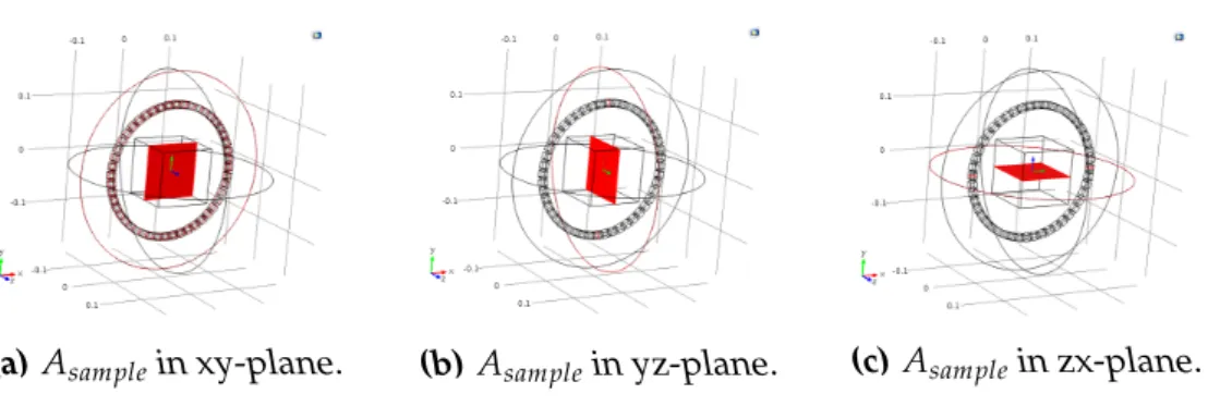
Usuallyηis expressed in parts per million (ppm). A field is completely homogeneous for η = 0 and gets more inhomogeneous for higher val-ues. To calculate the average magnetic flux < B >and variance< B2 >, surface integrals were taken of a square surface placed inside the magnet array (see Figure 2.11).

< B>= Z Z

Asample

B dA

<B2 >= Z Z

Asample

B2 dA

(16)

16 Theory

(a)Asamplein xy-plane. (b)Asamplein yz-plane. (c)Asamplein zx-plane.

Figure 2.11: Surface area of sample Asample in a plane (red) inside the magnet

array.

To calculate the inhomogeneity of the magnetic field in the xy-plane, yz-plane and zx-plane, a parametric sweep was taken for several values of surface areasA =Ssample2(see Figure 2.11. This way we can determine the maximum sample volume in which we can measure for a homogeneity below a chosen threshold (for example: η ≤10 ppm, 50 ppm, 100 ppm or 500 ppm). A field homogeneity below 10 ppm clinically used, but it is still useful to evaluate for these higher thresholds, as models may be improved later on.

2.3.1 Spatial resolution

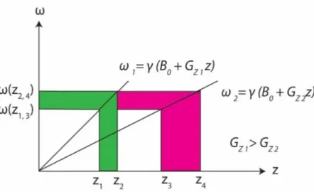
To obtain spatial information, in other words, to know where we’re mea-suring, we can apply three gradient fields using RF coils, each in a different direction. These gradient fields are magnetic fields that change linearly in one direction, resulting in small changes in the magnetic field strength, usually expressed in mT/m. A slight change in magnetic field will result in a small change in Lamor frequency:

ω0(z) = γ~B=γ(B0+Gz z) (2.18)

whereB0is our homogeneous magnetic field, andGzis the applied gradi-ent (see Figure 2.12).

This study is however primarily focussed on making a homogeneous

B0 field and applying a RF pulse to obtain spin proton information, and

will not explore using RF pulses for gradient fields. We can however use the inhomogeneity of ourB0field as a gradientB0(x) = B0+Gx, provided

Gx is more or less linear. Using this gradient we can determine what kind of spatial resolution we might expect in the MRI image. We can determine the slope of the gradient of our magnetic field by taking its derivative in

16

(17)

2.3 Simulating the magnetic field 17

Figure 2.12: Gz1 and Gz2 are two gradients, Gz1 having a higher slope. We can

see that a higher gradient results in a thinner slice (z1−z2) if we use the same

bandwidth∆ω= ω(z2,4)−ω(z1,3), which should be centered around the Lamor

frequencyω0. [6].

the direction:

Gx = dB0

dx Gy = dB0

dy Gz = dB0

dz (2.19)

If the slope of G is constant, we can expect slices with constant thick-ness T. In this slice, we can expect proton spins to have a precession fre-quency in the domain[ω0−∆ω, ω0+∆ω], also called the bandwidth. We

can select a slice by sending a RF pulse (to tip the spins of the protons) with a bandwidth equal to this. The slice thickness T is given by:

Tx = 2∆ω

γGx (2.20)

with∆ωthe bandwidth of the applied RF pulse.

2.3.2 Safety

(18)

18 Theory

or atleast produce artefacts in the image. In Low Field MRI, we work with less powerful magnetic fields, but we should still consider the safety regulations. In public spaces the stray magnetic field should not exceed 5 Gauss (0.5 mT), as it could be dangerous for people with for example pacemakers [19]. Therefore it is also important to simulate the stray mag-netic fields, so we can take the right precautions, such as using shielding techniques such as placing the scanner inside a Faraday Cage [19].

2.3.3 Robustness model

If we want our MRI model to be portable, it should also be able to some-what robust, and withstand external forces and environmental influences. Field homogeneity can be affected by change in the magnet’s magnetisa-tion direcmagnetisa-tion, remanence strength, volume or temperature. Our simula-tions use remanence strength to solve Maxwell’s equasimula-tions, so we will fo-cus on that. A change in magnetic remanence expresses itself in a change in total magnetisation of the magnet. The magnetic remanence itself does not really change over time [20], but the resulting magnetisation of the magnet be changed abruptly by for example a change in volume. Falling damage or other collision damage can make a dent in the magnet or chip a part off, reducing the total magnetisation of the magnet. A second thing to consider is the forces that these magnets act on each other. The direction of the magnetisation is different for each magnet, and neighbouring mag-nets would like to align themselves in the same direction, which produces a force on the casing they are in. If these forces are too great, the casing might break, and our model will be destroyed. Therefore it would also be interesting to simulate and calculate the magnetic force that these magnets exert on each other. This magnetic force can be represented as the torque, τ, on the magnet:

~τ =~µ×~B (2.21)

where~µ is the magnetisation of the magnet, and~Bis the magnetic field it is in [18]. To calculate it, it is useful to separate the magnet in small parts with magnetisationµ, calculate the torque on each part and sum it up.

2.4 RF transmitting and receiving

To get a Magnetic Resonance signal, we need to send a large RF pulse to flip the spins of the protons inside the sample. This causes change in net magnetisation, which we can measure via inductance in a RF resonant coil

18

(19)

2.4 RF transmitting and receiving 19

placed around the sample. This signal is called the Free Induction Decay, or FID (see Figure 2.13)

Figure 2.13: Free Induction Decay measured via induction due to change in net magnetisation of the proton spins.

(20)

(21)

Chapter

3

Methods and results

To design and simulate several magnet array designs commercial physics simulation software, COMSOL Multiphysics v5.2, was used. COMSOL uses a finite element method (FEM) with a user-defined mesh to solve for all kind of scientific and engineering problems in special modules (e.g. Electromagnetism, Structural & Acoustics, Fluid & Heat, Chemical) and specializes in coupling different kind of physics modules in one model. First we will show measurements of the magnetic field of a Halbach array already made in the lab, and simulate it, so we can check if our simulations hold up to reality.

3.1 Measuring the Magnetic flux field

We can compare our simulated magnetic field with the ’real’ magnetic field, which we measured by placing a Hall-effect probe in several points of a roster, placed in the middle of the magnet array (see Figure 3.1).

(22)

22 Methods and results

Figure 3.1: Picture of a Halbach circular array. The black arrows indicate the direction of magnetisation of each magnet. We placed a roster inside the array, to measure the magnetic field at fixed points using a Hall-effect probe.

3.2 Simulating a Halbach array

The magnetic field generated by ferromagnets was simulated in COMSOL using the ’Magnetic Field, No Currents’ module and solves Maxwell’s equations for no currents (see equations (2.11)-(2.15)).

Each permanent magnet has a magnetic remanence in a fixed direction, as required for e.g. a Halbach array (see Figure 2.7). This model is only valid if the ferromagnets don’t influence each other too much, in other words, if the magnetic field that the magnet ’feels’ is less than it’s intrinsic coercitivity [21], [22]. If the field is too strong, then the magnet gets mag-netized in the direction of the strong magnetic field, and the array does not satisfy the Halbach requirements any more. A typical Neodynium magnet, which we use in our models, can have an intrinsic coercivity of as high as 3.2T, which is much higher than the generated magnetic fields (B0 <1T), so our approach is justified [21].

22

(23)

3.2 Simulating a Halbach array 23

A previously made circular Halbach array was simulated in COMSOL. The array consists of 48 square magnets, of 12 x 12 x 10 mm size (length x width x depth) and magnetic remanenceBr = 1.2T, spaced in a circular array with radius 12.2 cm. The resulting magnetic field is mainly in the y-direction, as we would expect from this Halbach array. A figure of this model in COMSOL can be seen in Figure 3.2.

Figure 3.2: Circular Halbach Array of 48 ferromagnets each 12 x 12 x 10 mm (length x width x depth), with magnetic remanenceBr =1.2T. The large kube in

the middle is the sample with volumeVsample =Skube3.

The magnetic field in the center of the array, from this point on denoted byB0 is simulated to beB0 = 0.00539T. We can compare this to the

mea-sured field of an already made array in the lab: B0 = 0.0063 T. We can

explain this difference in three ways: Firstly the remanence of the mag-nets could be off due to a fabrication error (errors may exist up to 10% in remanence). Secondly our Hall-effect probe was very sensitive to minor changes in rotation and position, which could mean we did not measure exactly in the center of the Halbach array. Thirdly there could be some en-vironmental influences, such as the 7T MRI scanner very near to the lab. Still, we are 17 % off and we are in the right order of magnitude.

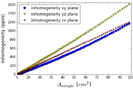
A parametric sweep for surface area Asample = Ssample 2 with Ssample from 0.1 cm to 10.0 cm with steps of 0.1 cm was taken in order to calculate the inhomogeneityη of the magnetic field.

(24)

Figure 3.3: Inhomogeneity ofBy field in xy-, yz- and zx-plane of N=48 Halbach

array.

planes: xy (blue squares), yz (yellow triangles) and zx (red stars).

To take some safety concerns into account, we also simulate the stray magnetic field, see Figure 3.4. In Figure 3.4a the magnetic field strength is plotted against the distance from the magnet array, starting from the outer edge of the magnet array, going outwards in the x-direction (red) and y-direction (blue). In Figure 3.4b the stray field is plotted against the distance from the center of the magnet, going outwards in the z-direction. To give some perspective, the radius of the Halbach ring is annotated at distance 12.2 cm (Rh), and the 50 Gauss and 5 Gauss lines are plotted.

24

(25)

3.3 Cylinder array 25

(a) from magnet array in x- and y-direction.

(b)from center of array in z-direction.

freespace

Figure 3.4:Strength of Stray Magnetic Field of N=48 Halbach array.

3.3 Cylinder array

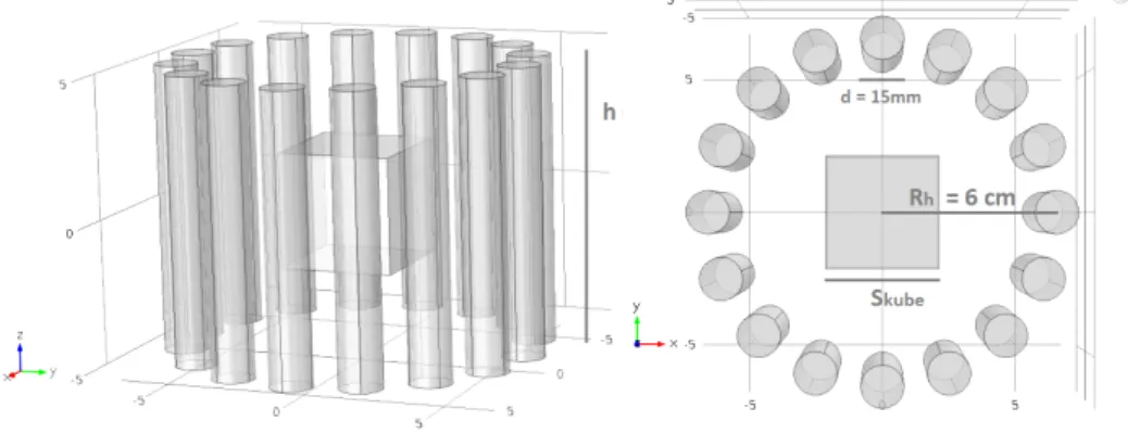
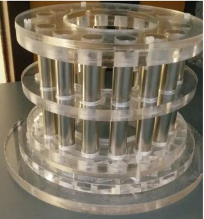
In order to compare Halbach arrays with other models, a cylinder magnet array was simulated, consisting of 16 cylindrical magnets with 7.5 mm radius and 100 mm height and remanence Br = 1.2T in the z-direction, placed in a circular array with 6.0 cm radius. A picture of this model can be seen in Figure 3.5.

(a)Side view of Cylinder array (b)Top view of Cylinder array

Figure 3.5: Magnet Array of 16 Cylinder magnets each 10 cm in length and 15 mm in diameter, withBr=1.2T.

(26)

the last two didn’t fit in the PMMA fitting at the end of construction (see Figure 3.6).

Figure 3.6:Picture of N=14 Cylinder Array.

To determine the effect of the last two cylinder magnets missing, and to still compare the simulated and real field, both the N=16 and N=14 model was first simulated and the inhomogeneity was calculated (see Figure 3.7 and Figure 3.9). The center field strengthB0of these models are for N=16:

B0 = 0.0578 T and for N=14: B0 = 0.0506 T. The center field of the N=14

Cylinder array was also measured with a Hall-effect probe: B0 =0.0051 T,

which is really close to the simulated value.

26

(27)

3.3 Cylinder array 27

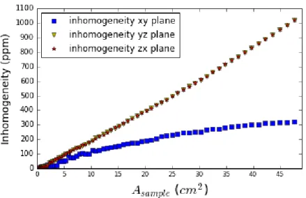
Figure 3.7: Inhomogeneity ofBz field in xy-, yz- and zx-plane of N=16 Cylinder

Array.

We can see the scatterplots of the inhomogeneity in the yz- and zx-plane completely overlap. This is logical, as the magnetic field is mainly in the z-direction and the magnet array is completely symmetrical in the x- and y-direction. The simulated strength of the stray magnetic field is shown in the line graphs (Figure 3.8).

freespace

(28)

Next we simulated the magnetic field of the N=14 Cylinder Array and calculate its inhomogeneity (see Figure 3.9) and the strength of the stray magnetic field (see Figure 3.10).

Figure 3.9:Inhomogeneity in xy-, yz- and zx-plane of N=14 Cylinder Array.

We can see that removing 2 magnets result in a lower center field strength and a more inhomogeneous magnetic field (especially in the zx-plane).

freespace

Figure 3.10: Strength of Stray Magnetic Field of N=14 Cylinder Array. To give some perspective, the radius of the array is annotated at distance 6.0 cm (Rh).

28

(29)

3.4 New Halbach array 29

3.4 New Halbach array

Next we want to make our own circular Halbach array model. We have to consider a couple of things in order to decide the dimensions of the model, as the array should not be too small, as we want to be able to make MRI scans of a child’s head inside the array, but it should also not be too big, as the field strength and homogeneity will decay with increasing the array radius. To compensate this, a larger model with more magnets can be used, but then the weight and cost will also increase. For our Halbach array we decide to fix some parameters. The radius of the Halbach array will be Rh = 7.5cm, as a child’s head will then fit inside it. We will use the strongest Neodynium magnets, 52NdFeB, with magnetic remanence

Br = 1.43T with length×width×depth = 25×25×25(mm). For a Hal-bach Array with radius Rh = 7.5cm we can use maximum 12 magnets (N=12). A model with fewer magnets, N=8, will also be evaluated, so we can compare their magnetic field strength and homogeneity. Models with

N < 8 were considered, but generated too weak magnetic field and poor homogeneity, as the Halbach array approximation does not hold up well for too few magnets. A picture of a N=12 Halbach array can be seen in Figure 3.11.

Figure 3.11:N=12 Halbach Circular array model in COMSOL.

(30)

its stray field (see Figure 3.13. The center field was simulated to be B0 =

0.0497 T.

Figure 3.12:Inhomogeneity in xy-, yz- and zx-plane of N=8 Mandhala.

(a)in x- and y-direction. (b)in z-direction.

Figure 3.13: Strength of Stray Magnetic Field of N=8 Halbach array. In b) the stray field is past the point ’Rh’ (radius of the Halbach ring).

30

(31)

3.4 New Halbach array 31

And now we do the same for the N=12 Halbach array (Figure 3.14) and it’s stray field (Figure 3.15). The center field was simulated to beB0 =

0.0746 T.

Figure 3.14:Inhomogeneity in xy-, yz- and zx-plane of N=12 Mandhala.

(32)

3.5 Double Halbach ring array

To increase the homogeneity of a circular Halbach array, we can add an-other Halbach ring, spaced at a certain distance d from the first ring. We will use two N=12 Halbach rings. See Figure 3.16 for a visualisation of this model.

Figure 3.16: Double Halbach ring array model in COMSOL, with distance d be-tween the rings.

In order to decide the ideal distance d, several simulations for different distances d were taken for a constant sample volumeAsample =36cm2. The inhomogeneity was calculated again in the three planes, as seen in Figure 3.17:

32

(33)

3.5 Double Halbach ring array 33

Figure 3.17: Inhomogeneity in xy-, yz- and zx-plane for different values of dis-tance between the rings of the Double Halbach, for constant sample volume

36cm2_.

(34)

Figure 3.18: Inhomogeneity of By of the Double Halbach array in xy-, yz- and

zx-plane for distance between the Halbach rings d = 5.25 cm.

The simulated center magnetic field isB0 =0.1118 T. In Figure 3.18 we

can see that the inhomogeneity in the xy plane stays below 100 ppm for a sample size up to 36cm2.

Figure 3.19:Strength of Stray Magnetic Field of Double Halbach ring array with d = 5.25 cm. In a) the stray magnetic field is plotted starting just outside the radius of the Halbach ring, between the rings (z=0). In b) the point ’Rh’ is annotated, which is the radius of the Halbach ring + d/2, to give some perspective.

Next for d = 5.95 cm the homogeneity was calculated (see Figure 3.20), and the stray field simulated (Figure 3.21). The simulated center magnetic field isB0 =0.1036 T.

34

(35)

We can see for d = 5.95 cm the inhomogeneity of the field in the zx-plane is lower than before (see Figure 3.18 and 3.20).

(36)

And lastly for d = 6.45 cm the homogeneity was calculated (see Figure 3.22), and the stray field simulated (Figure 3.23). The simulated center magnetic field isB0=0.0977 T.

We can see that for d = 6.45 the inhomogeneity in the zx-plane stays low even longer than at d = 5.95 cm (see Figure 3.20 and 3.22).

Figure 3.23:Strength of Stray Magnetic Field of Double Halbach ring array with d = 6.45 cm. In a) the stray magnetic field is plotted starting just outside the radius of the Halbach ring, between the rings (z=0). In b) the point ’Rh’ is annotated, which is the radius of the Halbach ring + d/2, to give some perspective.

36

(37)

The previous simulations were all done with sample volume 36cm2. To check if this is consistent with other sample volumes, the same simula-tions were done for sample volume 9cm2 (with sides 3.0 cm) and 2.25cm2

(with sides 1.5 cm). The simulated inhomogeneity as a function of distance between the rings is shown in Figure 3.24 and 3.25.

Figure 3.24: Inhomogeneity in xy-, yz- and zx-plane for different values of dis-tance between the rings of the Double Halbach, for constant sample volume9cm2.

Figure 3.25: Inhomogeneity in xy-, yz- and zx-plane for different values of dis-tance between the rings of the Double Halbach, for constant sample volume

(38)

We can see that the minima for the inhomogeneity in the three planes get closer to each other for smaller sample volume (see Figure 3.17, 3.24, 3.25). In Figure 3.24 we can see the three minima for d = 5.95 cm (in xy-plane, which we already found in Figure 3.17), d = 6.15 cm (in yz-plane) and d = 6.25 cm (in zx-plane). In Figure 3.25 we can see the minima get closer even more and almost overlap around d = 6.15 cm. To further ex-plore this, the inhomogeneity of the generated B field was also calculated for d = 6.15 cm and d = 6.25 cm for different sizes of sample volume (see Figure 3.26 and 3.27).

38

(39)

3.6 Spatial Resolution 39

This model has center field strength ofB0 =0.1012 T.

This model has center field strength ofB0 =0.1000 T.

We can see that for d = 6.15 and d = 6.25 cm the homogeneity in the zx-plane improves greatly and in the xy- and yz-plane it improves a little.

3.6 Spatial Resolution

(40)

(a) (b)zoomed in.

Figure 3.28:Gradient ofByof N=12 Halbach array in x-, y- and z-direction.

We can see in Figure 3.28 that the gradient Gx and Gy are at no point constant, but Gz is more or less constant for distance 2.50 - 3.50 cm from the center withGz =11.67±0.23 mT/cm.

From these gradients Gx, Gy, Gz we can calculate the resulting slice thicknessTx,Ty,Tz, after we choose the bandwidth of the RF pulse. Hockx proposes it to be ∆ω = 1MHz and built a probe that is resonant in this frequency range [13]. For consistency, we also choose∆ω =1MHz. From Eq. 2.20 we can then can calculate the slice thickness:

Figure 3.29:Slice thickness T in x-, y- and z-direction for N=12 Halbach array.

We can indeed see that Tzstays constant for distance from center from 2.50 - 3.50 cm with Tz = 0.32±0.01 cm, calculated using the average(T) and sigma(T) of T in this domain. We can also see that there is no point of using the gradient of the magnetic field for distances very close to the center, as the slice thickness gets really large, in the order of the sample size.

40

(41)

We can repeat the same process for the Double Halbach ring Array. For distance between rings d = 5.25 cm we find:

Figure 3.30:Gradient ofByof the Double Halbach array in x-, y- and z-direction.

and slice thickness:

Figure 3.31:Slice thickness T in x-, y- and z-direction.

We can see that at no point the gradients are constant, and conse-quently the slice thickness also is not constant. For small distances from the center (up to 2.0 cm) the gradient stays very low: below 2.5 mT/cm.

(42)

Figure 3.32:Gradient ofByof the Double Halbach array in x-, y- and z-direction.

Figure 3.33:Slice thickness T in x-, y- and z-direction.

We can see that we get comparable results. The gradients are again at no point constant and for small distances (up to 2.0 cm) very low. The resulting slice thickness is for distances ≤ 2.0 cm very large (up to 100 cm), thus using the gradient of the magnetic field is not usefull. Further away from the center (≥3.0 cm) the slice thickness gets reasonably small:

Ty =0.21±0.11 cm andTz =0.40±0.09 cm, but still not constant, hence the high sigma).

42

(43)

3.7 Robustness Magnets in model 43

3.7 Robustness Magnets in model

To simulate damage to the model, we decreased randomly the magnetic remanence of 1, 2 resp. 3 magnets in the N=12 Halbach model. We cal-clated the inhomogeneity of the magnetic field for 3 times, for different randomly chosen magnets, and averaged the result. The change in homo-geneity can be seen in Figure 3.34.

(a)1 magnet -10 %Br (b)2 magnets -10 %Br

(c)3 magnets -10 %Br

Figure 3.34:Influence of -10%Brin 1, 2, 3 magnets at random (a, b, c).

We can see that we can expect at least a∆η =10 ppm, which increases with the number of magnets that have reduced remanence, up to ∆η = 22.5 ppm.

Unfortunately we were not able to simulate the influence of temper-ature on the homogeneity of the produced magnetic field, nor the forces that the magnets act on each other.

3.8 RF Transmit and Receive switch

(44)

(and receive) frequencies ranging from DC to RF with voltage≤1V. A 1V RF pulse is too small, so we need to amplify the pulse to let it have higher voltages (e.g. 50V). We use open-source software GNU-radio to control the USRP1. We can control what kind of pulses (DC or RF) to transmit and during what time (pulsewidth) and with a transmit rate TR. A sketch of our setup can be seen in Figure 3.35.

Figure 3.35: Figure of our setup. When we transmit the RF pulse from Tx1, it

gets amplified by the amplifier and mostly goes into the Coil. To prevent it from damaging the receiverRx1we place a passive filter, which attenuates the signal

below 1 V, and an active filter, which attenuates it even more. The FID is in the order of mV), so we need a Pre-Amp to amplify it, so we can measure it.Tx2sends

out a DC signal to the DC-driver, which turns the active filter on and off.

3.8.1 Software

To control the USRP1 we use open-source software GNU-radio. We can generate DC and RF signals by defining and connecting several blocks. We used the program in Figure 3.36, made by J. Hockx.

3.8.2 Passive Filter

Our passive filter is based upon the design of J. Hockx [13], who based his design on the filter design of Lowe and Tarr [24]. Lowe and Tarr use two sections of crossed diodes and aλ/4 between the probe and receiver.

The Lamor frequency for 0.1T magnetic field results in a very largeλ, in the order of 10 meters), so using aλ/4 is impractical. Hockx replaced it with a Pi-section filter, which acts the same as aλ/4 cable. The Pi-section

44

(45)

3.8 RF Transmit and Receive switch 45

Figure 3.36: GNU-radio program by J. Hockx [13]. In this diagram two signals are generated: a RF pulse and a DC pulse. The DC pulse is our TTL signal to drive our active filter.

filter consists of two capacitors and a inductor, such that the resonance frequency of the circuit is the Lamor frequencyω0=1/

√

LC.

Placing several passive filters in series increases the attenuation of the signal, but also increases the noise generated by this circuit. Also, no mat-ter how many passive filmat-ters you put in series, the output voltage will always be of the order ofVf wof the diodes [13].

3.8.3 Active Filter

Our active filter mainly consists of a PIN-diode. A PIN-diode is very help-ful in RF circuits as a switch, because it has very low intrinsic impedance for RF signals and can be controlled by a DC signal. If we apply a DC signal ≥ Vf w then it completely conducts and the signal from Uin gets diverted through the PIN-diode towards the ground.

(46)

Figure 3.37: Sketch of Lowe and Tarr’s passive filter. The crossed diodes at A allow a RF pulse to travel through to the sample in the probe as its voltage is higher than the forward voltage of the diodesV_{f w}, and prevent the FID signal to go through the transmitter, as its voltage is lower thanVf w. Theλ/4 and

protec-tion diodes placed at B attentuate the RF pulse, as its diverted to the ground (at Diode short). The FID signal from the sample will be less attenuated, as its volt-age is lower thanVf wand does not get diverted towards the ground and reaches

the receiving end.

Figure 3.38:Hockx’s passive filter. The Pi-section filters acts as aλ/4 section. As

in Lowe and Tarr’s circuit (see Figure 3.37), the crossed diodes direct most of the RF pulse towards the probe, and the FID signal towards the receiver.

apply a lower voltage.

In collaboration with the Electronische Dienst (ELD) of Leiden Uni-versity and J. Hockx, we came up with a circuit that correctly drives the PIN-diode (see Figure 3.40). Our DC driver circuit consists of an invert-ing Op-Amp, opa627, with high recovery time (8 ns), two 1N4148 diodes with Vf w = 0.6V and a Zener 2V4 diode. The Op-Amp gets powered by

46

(47)

Figure 3.39: Sketch of the active filter. The two capacitors beside the PIN-diode prevent the DC signal from the DC driver from influencing the RF signal, as ca-pacitors have very high impedance for DC signals. The inductor in front of the DC driver prevents RF signal from entering the DC circuit, as inductors have very high impedance for high frequency signals.

V+ and V-. The upper diode limits the positive output voltage to +0.6V (which turns the PIN-diode off), and the Zener diode caps the negative output voltage to -2.4V. The diode to the left of the Zener diode prevents V+ from entering the Op-Amp circuit. R1limits the current that can enter

our system, to protect the Op-Amp.

(48)

Figure 3.41: Sketch of input and output of the DC driver. The input is a TTL signal with OFF = -0.5V and ON = +0.5V, which results in a output of +0.6V for OFF and -2.4V for ON, which correctly lets the PIN-diode block signal for OFF and completely conduct and divert the signal to the ground for ON.

To check if our switch works properly, we send a RF pulse through it, with a DC signal to the DC driver. We get the following images if we connect the output to an oscilloscope (WaveAce 234).

48

(49)

(a)RF pulse through the circuit (blue). Here the signal is only attenuated by the passive filter, as the DC signal to the DC driver is off, to around 500 mV, which is theVf wof the crossed diodes.

(b) RF pulse through the circuit. The yellow square wave is the applied DC signal to the DC driver. We can see the active filter is on, as the signal is atten-uated even more, to around 200mV.

(c)RF pulse, also outside of the DC sig-nal. Here we can see that if we allow the RF pulse through the circuit while the switch is off (to the right of the yellow square wave), the signal is still strongly attenuated.

Figure 3.42: Influence of the passive and active filters on the RF pulse (blue) through our setup.

(50)

in the circuit and corrected it. If we connect the output to the oscilloscope we can see the reaction of the circuit to a RF pulse and a DC signal, see Figure 3.43

Figure 3.43:We apply a continuous RF signal through the passive and active filter. We can see the output RF signal in red, the applied DC signal to the DC driver in yellow, and the output of the DC driver in green.

We can see that the RF pulse gets strongly attenuated if the switch is ON (green square wave is at -3V) and is less attenuated if the switch is off (green square wave at 0.6V), which is exactly what we would expect. However, we see that the reaction of the RF signal just after switching gives us a peak in signal. This is referred to as spectral leakage [25].

50

(51)

Chapter

4

Discussion

We can see our simulations give similar values for center magnetic field strength for the N=48 Halbach array (error 17 %) and N=14 Cylinder ar-ray (error 1 %), but we need to make more comparisons to evaluate this properly. We were not able to compare the calculated homogeneity of the magnetic field from the simulations with the measured field of a already made model. We advice a more rigid and consistent Hall-effect probe, so that differences in magnetic flux field can be measured consistently and accurately. Using a Robotic arm from for example a 3D printer can greatly improve spatial resolution in measuring the magnetic field and the homo-geneity of the magnetic field can be calculated properly.

We can evaluate the simulated models for center field strength B0,

ho-mogeneity η, sample volume Vsample, safety and robustness, and spatial resolution. Lastly the costs and weight of the total setup will be given.

First lets compare the maximum sample volume (length x width x depth) incm3for field inhomogeneity below a chosen threshold.

Halbach Cylinder

η(ppm) N=48 N=12 N=8 N=16 N=14

100 2.8 x 3.2 x 2.6 2.0 x 1.5 x 1.6 2.0 x 1.5 x 1.6 2.3 x 3.0 x 2.3 2.7 x 2.2 x 2.4 200 4.0 x 4.5 x 3.6 2.7 x 2.2 x 2.4 2.7 x 2.2 x 2.4 3.2 x 4.6 x 3.2 4.2 x 3.1 x 3.3 300 4.9 x 5.4 x 4.4 3.3 x 2.7 x 3.0 3.3 x 2.7 x 3.0 3.9 x 6.3 x 3.9 5.4 x 3.8 x 4.1 500 6.3 x 6.9 x 5.7 4.2 x 3.5 x 3.8 4.2 x 3.5 x 3.8 5.0 x 7* x 5.0 7* x 4.8 x 5.2 1000 9.0 x 9.3 x 7.9 5.7 x 4.9 x 5.5 5.5 x 4.9 x 5.5 6.8 x 7* x 6.8 7* x 6.6 x 7*

(52)

52 Discussion

From this table we can calculate the sample volume, minimum for a cubic sample (equal sides), maximum for a box with unequal sides.

V_sample Halbach Cylinder

η(ppm) N=48 N=12 N=8 N=16 N=14

max min max min max min max min max min

100 23 18 5 3.4 5 3.4 16 12 14 11

200 65 47 14 11 14 11 43 30 47 33

300 116 85 27 20 27 20 84 55 96 59

500 248 185 56 43 56 43 175* 125 174* 111

1000 661 493 154 118 148 118 324* 314 323* 287

Table 4.2: Max. sample volume (box shaped) and min. sample volume (cube shaped) of each array. ’*’ indicates that the max sample side length of 7.0 cm was reached withηbelow the threshold.

(a)Min.Vsamplewith equal sides (cubic). (b)Max. Vsamplewith unequal sides.

Figure 4.1:Min. and max.V_samplefor chosen thresholds of homogeneity.

We can see from this table that the N=48 Halbach can support higher volume samples forη ≤a chosen threshold (roughly 5 times larger) than the N=12 and N=8 Halbach arrays. On the other hand, we should also take the center magnetic fieldB0into consideration:

Model B0(T)

Halbach N=48 0.0054 N=12 0.0746 N=8 0.0497 Cylinder N=16 0.0569 N=14 0.0498

52

(53)

4.1 Double Halbach Ring array 53

Table 4.3:Center magnetic field strengthB0.

We can see that in terms of highest center field strength, the N=12 Hal-bach ring array is clearly the winner, with a center field strength B0 more

than 10 times stronger than of the N=48 Halbach array.

4.1 Double Halbach Ring array

We can see that choosing different values for the distance between the Halbach rings effects the homogeneity of the magnetic field, especially in the xy-plane (see Figure 3.18) and in the zx-plane (see Figure 3.22). So by choosing a sample volume, and in which plane to measure, we can optimise field homogeneity by choosing the correct distance between the rings. The center magnetic field strengthB0for different distances is:

Double Halbach

d (cm) B0(T)

5.25 0.1118

5.95 0.1036

6.15 0.1012

6.25 0.1000

6.45 0.0977

Table 4.4:Center Magnetic field strengthB0.

Increasing the distance between the rings also decreases the center field strength B0, but it stays around 0.1T.

η(ppm) d=5.25 d=5.95 d=6.45

10 1.4×1.0×1.1 3.5×2.1×2.2 1.9×1.8×2.2 20 1.9×1.5×1.6 3.9×2.7×2.9 2.6×2.4×4.5 50 3.3×2.3×2.5 4.5×3.5×4.0 3.5×3.3×4.7 100 6.1×3.3×3.5 5.2×4.3×5.1 4.3×4.1×5.8 200 6.7×4.5×4.8 5.9×5.2×6.3 5.2×5.0×7.0 300 7.0×5.3×5.7 6.3×5.8×7.0 5.7×5.6×7∗ 500 7∗ ×6.4×7.0 6.9×6.7×7∗ 6.5×6.5×7∗

Table 4.5: Length of sample sides in plane (xy) x (yz) x (zx). Values for d are found by taking inhomogeneity minima for A_sample = 36cm2_{. ’*’ indicates that}

(54)

54 Discussion

From this table we can calculate the sample volume with inhomogene-ity below a chosen threshold. We can calculate the minimum sample vol-ume for a kubic sample (equal sides), and maximum sample volvol-ume for a box shaped sample with unequal sides.

Vsample d=5.25 d=5.95 d=6.45

η(ppm) max min max min max min

10 1.54 1.0 16.2 9.3 7.5 5.8

20 4.6 3.4 30.5 19.7 28.1 13.8

50 19.0 12.2 63.0 42.9 54.3 35.9

100 70.5 35.9 114.0 79.5 102.3 68.9

200 144.7 91.1 193.3 140.6 182 125

300 211.5 148.9 255.8 195.1 223.4* 175.6

500 313.6 262.1 323.6* 300.8 295.8* 274.6

Table 4.6: Max. sample volume (box shaped) and min. sample volume (cube shaped) of Double Halbach array. ’*’ indicates that the max sample side length of 7.0 cm was reached withηbelow the threshold.

We can also do this for the values for d found by takingAsample =9cm2 (see Figure 3.24 and 3.25).

η(ppm) d=6.15 d=6.25

10 2.9×2.3×2.9 2.5×2.3×3.0 20 3.3×2.8×3.6 3.1×2.8×3.9 50 4.1×3.6×4.6 3.9×3.6×4.7 100 4.8×4.3×5.5 4.6×4.3×5.7 200 5.6×5.2×6.7 5.5×5.2×6.8 300 6.1×5.8×7∗ 6.0×5.8×7∗ 500 6.7×6.7×7∗ 6.6×6.6×7∗

Table 4.7: Length of sample sides in plane (xy) x (yz) x (zx). Values for d are found by taking inhomogeneity minima forAsample = 9cm2. ’*’ indicates that the

max sample sideS_sample =7.0cm was reached withηbelow the threshold. 54

(55)

4.1 Double Halbach Ring array 55

Vsample d=6.15 d=6.25 η(ppm) max min max min

10 19.3 12.2 17.3 12.2

20 33.3 22.0 33.9 22.0

50 67.9 46.7 66.0 46.7

100 113.5 79.5 112.7 79.5

200 195.1 140.6 194.5 140.6

300 247.7* 195.1 243.6* 195.1

500 314.2* 300.8 304.9 287.5

Table 4.8: Max. sample volume (box shaped) and min. sample volume (cube shaped) of Double Halbach array. ’*’ indicates that the max sample sideSsample=

7.0cm was reached withηbelow the threshold.

We can already see a drastic increase in sample volume of the Double Halbach ring array (Table 4.6 and 4.8) of 6 to 12 times more than the single Halbach ring arrays (Table 4.2).

We can put the sample volume again into scatterplots to compare for different distance between rings d.

(a)Min.Vsamplewith equal sides (kubic). (b)Max.Vsamplewith unequal sides.

Figure 4.2:Min. and max.Vsamplefor chosen thresholds of homogeneity.

We can see that we get the highest sample volume for d = 5.95 cm, d = 6.15 cm and d=6.25 cm being a close second.

Still, the homogeneity of the magnetic field needs to be improved fur-ther, to get higher Vsample with low inhomogeneity (10 or 50 ppm). B0

(56)

56 Discussion

4.2 Stray Magnetic field

To take safety regulations into concern, the distance for the stray field to decay to≤5 Gauss (0.0005T) is given:

model\distance x (cm) y (cm) z (cm) Rh (cm)

Halbach N = 48 4.3 8.9 15.5 12.2

Halbach N = 12 5.8 9.8 19.4 7.5

Halbach N = 8 5.8 9.6 19.0 7.5

Cylinder N =16 39.4 39.4 41.2 6.0

Cylinder N =14 35.5 35.7 40.0 6.0

Double Halbach d=5.25 7.2 13.3 23.4 7.5, 10.125 Double Halbach d=5.95 6.9 13.0 23.5 7.5, 10.475 Double Halbach d=6.45 6.6 12.8 23.7 7.5, 10.725

Table 4.9:minimal distance from array required for stray magnetic field to decay

≤ 5Gauss (0.0005T). The distance in x- and y-direction are given going outward from the radius of the array, while the distance in z-direction is given going out-ward from the center of the array. In column ’Rh’ the radius of the array is given. For the Double Halbach array, also the length of the array plus the Halbach radius is given for perspective.

We can see that for the N=12 and N=8 Halbach array the minimal distance increases in the y- and z-direction with the number of magnets. There’s (almost) no change in the x-direction, most likely because the field in the x-direction is already very weak, as most of the field is pointed to-wards the y-direction. For the Cylinder Array we can see that adding 2 cylinder magnets increases the minimal distance, as expected because more magnets cause a stronger magnetic field. We can see that the mini-mal distance is lowest for the Halbach arrays, as is expected. The Double Halbach ring arrays have 1.2 larger minimal distance in x- and y-direction than the single Halbach ring arrays, which is logical, because the Double Halbach ring array has twice as many magnets, so a higher center field strength and is also d longer in the z-direction (see column ’Rh(cm)’). In-creasing d (distance between the rings) decreases the minimal distance in x- and y-direction, as the center magnetic field strength also decreases. In z-direction the minimal distance increases, which is logical because the array gets wider with increasing distance between the rings.

56

(57)

4.3 Spatial Resolution

Using the gradient of the magnetic field itself seems to be only useful for the N=12 Halbach array, and only in the z-direction, in a specific range (2.50 to 3.50 cm), as in that domain the gradient is constant, and conse-quently the slice thickness is constant. For the Double Halbach ring Array the gradient is at no point constant. For small distances from the center the slice thickness is too high to be usable (in the order of the sample size), but gets reasonably small (≤0.5 cm) after 3.0 cm. For small distances from the center an external gradient has to be used in order to acquire spatial information. An external gradient can be made using a quadruple Hal-bach array (m=2), or a dipole HalHal-bach array rotated with respect to theB0

magnet array, and should be explored further.

4.4 Robustness Model

If the magnetisation of 1 or more magnets is reduced, we can see that it has high impact on the homogeneity of the produced magnetic field (see Figure 3.34), in the order of 10 to 20 ppm. Protecting the model is thus of importance. We advice further research in the effects of change in temper-ature, change in shape of the magnets, and the magnetic force that mag-nets exert on each other to better evaluate the robustness of the models. Simulating en evaluating several shielding techniques to protect the mag-net array, and to limit its stray magmag-netic field, and experimenting with B0

shimming techniques to improve the homogeneity of the magnetic field is also valuable.

4.5 RF Transmit-Receive switch

(58)

58 Discussion

provide for a good basis to be able to detect a Free Induction Decay, if the probe was placed inside a strong magnetic field with a sample inside it. We advise further research to be done with an already functional MRI, such as the 1T, and make a proper probe, to test the circuit and try to get a FID. To make the setup more cost and space efficient, a small computer like a Raspberry Pi could be used to drive the USRP1 [26].

4.6 Costs and Weight

In this section the costs and weight will be estimated for the whole setup. The precise models used in our setup will be listed in the appendix.

For the magnet array, let’s assume we will use the Double Halbach ring array, so 24 N52 magnets 25x25x25 (mm), which will cost in total 500 and weight: 3 kg. Let’s assume we use a aluminium casing, which we estimate will cost 100 and weigh 5 kg. For the RF setup, let’s assume we use a Raspberry Pi.

model costs (e) weight (kg)

USRP1 700 1

RF circuit 25 1

Raspberry Pi 50 1

RF Amplifier 1.000 5

RF Pre-Amplifier 100 1

DC Power Supply 100 5

several cables (COAX) 50 1

24 magnets 500 3

magnet casing 100 5

total 2.625 23

Table 4.10:Estimated costs and weight of setup.

If we compare this to a conventional 0.1 T MRI, which is at least 100.000 eand 15.000 kg, we see that our system is 38 times cheaper, and 65 times lighter, and far smaller.

58

(59)

Chapter

5

Conclusion

We have shown that we can simulate several magnet array models, using COMSOL Multiphysics, which give comparable magnetic field strength with measured magnetic field strength using a Hall-effect probe. We can calculate the homogeneity of the produced magnetic fields and evaluate the models, where the Double Halbach ring array was shown to be the best in terms of field homogeneity and center field strength. The stray magnetic field was comparable with the single Halbach ring array, and far less than that of the Cylinder array, so we suggest this array to be used in portable MRI scanners. The Double Halbach ring array could also han-dle the largest samples for a chosen inhomogeneity threshold. We find the Double Halbach ring array is the best choice for producing theB0field, but

(60)

(61)

(62)

(63)

Appendix

A

Materials

Object Company Model

Software Defined Radio (SDR) ETTUS Research USRP1

RF Amplifier Electronic Navigation Industries 310 L

RF Pre-Amplifier MITEQ AU - 1054

DC Power Supply Tenma 72-10500

RF Wave Generator Agilent Technologies N9310A

Oscilloscope LeCroy WaveAce 234

Lasercutter VersaLASER Laser 2000

Gauss meter AlphaLab Inc. GM-2

(64)

(65)

Appendix

B

COMSOL Multiphysics

Presented in this chapter is a short guide on how to simulate ferromag-net models. We can make a model from scratch by first selecting ’Model Wizard’, and then ’3D’.

(a)Select ’Model Wizard’ _(b)_{Select ’3D’}

Figure B.1:Set up a new model.

We could also choose to solve in 2D axisymmetric to speed up the sim-ulations, but it is also harder to make the model in this set up.

B.1 Choose module

(66)

66 COMSOL Multiphysics

(a)Select ’mnfc’, ’Add’, and ’Study’ (b)Select ’Stationary’, and ’Done’

Figure B.2:Select Physics and type of Study.

B.2 Geometry

Setting up a simulation usually follows the same procedure, represented by the sections on the header, from left to right (see Figure B.4). We can start by selecting ’Geometry’ from the header, or from the menu on the left.

66

(67)

B.2 Geometry 67

(a) Right-click Geometry and add a cube, ’Block 1’

(b) In ’Size and Shape’ define width, depth and height of Block 1.

Figure B.3:Add a cube to the Geometry.

(68)

(a)Right-click Global Def-initions and Select ’Pa-rameters’

(b) Add parameter ’Scube’ with value

’5 [cm]’

(c)Use parameter ’Scube’ in ’Block 1’

freespaaacceee

Figure B.4:Add a parameter, define it and use it.

We can also change the position of the block in ’Position’. Let’s displace the block for 15 cm in the y-direction. This way the radius of our circular array is 15 cm. To make a circular array of several cubes, we can use the ’Rotate’ function in ’Transforms’ in the ’Operations’ tab of ’Geometry (see Figure B.5). We have to select an object on which we transform function ’Rotate’ will work. We want to make an array of blocks, so we have to select Block 1 by clicking on it in the Graphics window. The selection shows up in ’Input objects’ as ’blk1’, which is our cube.

Next we can choose how many objects the array should exist of by defining the rotation angle. If we want to have 8 magnets in our circular array, we have to rotate the cube in 8 steps, which we can implement by typing range(0, 45, 360) as rotation in ’Rotation Angle’, as 360/8 = 45.

68

(69)

B.2 Geometry 69

(a) Select the Transform function ’ro-tate’ in the Operations tab of Geometry

(b) Select Block 1 as target and define rotation properties

Figure B.5:Make a circular array of cubes.

(70)

(a)Circular array of 8 cubes (b)First cube is rotated another time

Figure B.6:Make a circular Halbach array of cubes.

The last thing that we need to do is make a sphere to define the space between the cubes. COMSOL uses a mesh to run its simulations and can not solve physics equations if there is empty space between objects. In the same way as making a cube, we can make a sphere and give it a radius. Two times the radius of the circular array seems adequate, so let’s use 30 cm. After clicking ’Build All Objects’, we can only see the sphere. If you still want to be able to see the circular array inside it, you can click the option ’Transparency’, the one but last option in the Graphics window (see Figure B.7).

B.3 Material Properties

Now we have made our geometry, we still have to define the material properties of each element. First we can give the sphere we just made the properties of air. First we have to add a material by right-clicking ’Materials’ and selecting ’Add Material’. This gives us a new menu ’Add Material’ to the right, where we can select ’Air’ under ’built-in’ by double-clicking it (see Figure B.7).

70

(71)

B.3 Material Properties 71

Figure B.7:Add material to Geometry, starting with Air

(72)

(a) Add material ’Air’ only to the sphere

(b)Resulting selection. Highlighted is the section with material properties

Figure B.8:Material ’Air’ added to only the sphere

In Figure B.8b we can also see all the material properties of air. For our simulations, mainly the relative permeability of materials is of impor-tance. Thus for the magnets, we can duplicate the material air, change the relative permeability to 1000, and apply it to all the cubes. The value 1000 is chosen after consulting multiple model examples from COMSOL and advice given by representatives. We can duplicate the material by right-clicking it and selecting duplicate. Now we have to select entity 2-9 in the selection box and change the relative permeability to 1000 (see Figure B.9).

Figure B.9: Duplicate material ’Air’, apply it to the cubes (2-9) and change the relative permeability to 1000.

72

(73)

B.4 Define physics 73

B.4 Define physics

The next step is to define the physics that we want to simulate. To add magnetic remanence to the cubes, we have to add a ’Magnetic Flux Con-servation’ to the mnfc module (see Figure B.10). Then we choose a cube, and select ’Remanent flux density’ as the constitutive relation and give it for example 1.3 [T] of magnetic remanence in the y-direction. We can do this for all the cubes by repeating this process. Be aware that for a Halbach array the direction of the magnetic remanence is not constant, but depends on the location of the cube in the array. I could not figure out how to make the remanence dependent on a angle parameter, e.g. θ, so I defined the magnetic remanence in polar coordinates:

Br,x =cos(n∗deltatheta)∗Br

Br,y =sin(n∗deltatheta)∗Br (B.1)

with Br = 1.3 T,deltatheta = 2π_N, with N the number of magnets and n ranging from 0 to N-1, depending on which magnet the ’Magnetic Flux Conservation’ law acts. So for the cube in Figure B.10 n = 0, for the next cube (to the right) n = 2, and so on. In total we have thus added N times the ’Magnetic Flux Conservation’ to the mnfc module to different cubes, and adjusted n accordingly.

(a) Add ’Magnetic Flux Conservation’ law to the mnfc module

(b) Select first cube and define mag-netic remanence

(74)

B.5 Apply Mesh

COMSOL uses a finite element mesh in order to simulate and calculate the different physics relations set up in the model. The mesh size is ’normal’ on default, but I advice to choose at least ’Extra fine’, as this gives better results. This however greatly increases the time needed to apply the mesh. Click ’Build All’ to finish applying the mesh. To gain more control over the mesh, you can select ’User-controlled’ in stead of ’Physics-controlled’ in the ’Sequence type’ of the mesh. It is also possible to define multiple meshes on different selections of the model by adding another mesh. This is handy if you’re mainly interested in one domain of the model, as you can make the mesh really fine in the interesting domain, and less fine in the rest of the domain. This is done by adding for example a ’Free Tetrahedral’ mesh twice, and defining the selection on which domains it should apply to and mesh element size accordingly.

B.6 Start study

When everything is set up, we can start the simulation by clicking ’Com-pute’ in the ’Study’ section, either in the header, or in the menu to the left. When it is done, we immediately get a default plot of the magnetic flux density in our model. We can see if we rotate the model in the graphics window (by holding the right mouse button) that we succeeded in giving magnetic remanence to a cube, as it produces magnetic flux around it. This plot can be found in the results section (see Figure B.11).

(a)Start simulation. (b)Add Parametric Sweep.

Figure B.11

74

(75)

B.7 Results and Evaluation 75

We can simulate several models by adding a ’Parametric Sweep’ in the Study section. A Parametric Sweep starts a study for different values of a chosen parameter. We can add a parameter by clicking on the plus sign. We only have one parameter now, ’Scube’, so it selects it by default. We can make several simulations for different sizes of magnets by inputting some values in the Parameter value list, for example 1, 2, 3 [cm]. (see Figure B.11). This way we can easily simulate several models at a time. Click ’Compute’ again to perform the Parametric sweep.

B.7 Results and Evaluation

When the Study is finished running we have acquired data in the ’Re-sults’ section. The data is given in a data set, by default ’Study 1/Solu-tion 1 (sol1)’ which tells us the data is acquired from performing Study 1, which is the stationary study we began with. For the Parametric sweep the dataset is called ’Study 1/Parametric Solutions (sol2)’. If we want to see the data only in the domain of the magnets, we can add a selection to the dataset by right clicking on it and choosing ’Selection’ (see Figure B.12). In the selection menu we can change the ’Geometry entity level’ to domain and select a cube (by either clicking on it on manually, or defining it in ’Paste Selection’). Now we have limited the dataset to only the data in the domain of the selected cube. This is particularly helpful if we want to evaluate the data in a chosen domain.

(a) (b)