Bernardi_unc_0153D_18086.pdf

SPACE/TIME EVOLUTION IN THE PASSIVE TRACER PROBLEM

Francesca Bernardi

A dissertation submitted to the faculty at the University of North Carolina at Chapel Hill in partial

fulfillment of the requirements for the degree of Doctor of Philosophy in the Department of

Mathematics in the College of Arts and Sciences.

Chapel Hill

2018

ABSTRACT

Francesca Bernardi: Space/Time Evolution in the Passive Tracer Problem

(Under the direction of Roberto Camassa and Richard M. McLaughlin)

This dissertation is concerned with understanding how the behavior of a concentration of tracer

undergoing an advection-diffusion process in Poiseuille flows depends on the pipe cross-section.

Per la mia famiglia,

che ha sostenuto e incoraggiato il mio desiderio di ottenere l’ennesimo

foglietto, nonostante la distanza.

Per mia madre,

che mi ha insegnato a sognare, ad andare per la mia strada, e a non

guardarmi indietro.

ACKNOWLEDGEMENTS

I owe a huge debt of gratitude to my advisors Roberto Camassa and Rich McLaughlin without

whom I would have never had the chance of becoming a graduate student at UNC. I live the life

I have always wanted because of them. I learned tough lessons working with them, both in and

outside Mathematics. These five years have been a wild ride, but have made me into a researcher.

I need to acknowledge the mentorship, friendship, and support that Dan Harris has given me

throughout the years. He taught me everything I know about experiments and so much more; I

learned about myself in the process.

I am also extremely grateful to Nuch Aminian, who has been my research partner from the

beginning and my guide through the impervious world of numerical simulations. We managed to

produce more quality work together than anyone else in our circumstances. We also became good

friends, arguably an even better accomplishment.

My time as a graduate student would have been much less rewarding without Katri Morgan.

Together we made things happen that I had only dreamed of. The time and effort we invested had

much better returns than we had hope. She became my friend and reliable partner and I hope our

collaborations will continue in the future, no matter where we end up.

Enrolling in the graduate certificate in Women’s and Gender Studies has been one of my best

decisions. It helped me find my voice, a voice I will never get tired of using now that I know how.

TABLE OF CONTENTS

LIST OF FIGURES . . . .

xi

LIST OF TABLES . . . xiii

CHAPTER 1: INTRODUCTION . . . .

1

CHAPTER 2: THEORETICAL BACKGROUND . . . .

4

2.1

The Advection-Diffusion Equation

. . . .

4

2.2

Taylor Dispersion . . . .

6

2.2.1

Poiseuille Flow . . . .

6

2.2.2

Dispersion by Advection Alone . . . .

8

2.2.3

Effect of Molecular Diffusion on Solute Dispersion

. . . .

9

2.2.4

Effect of Using Condition (B) . . . .

10

2.2.5

Experimental Procedures

. . . .

12

2.3

Aris’ Generalization of Taylor’s Coefficient . . . .

15

2.3.1

The Péclet Number . . . .

16

2.4

The Moments Expansion Method . . . .

17

2.4.1

Longitudinal Moments . . . .

18

2.4.2

Skewness

. . . .

18

2.5

Moments Expansion of the Concentration . . . .

19

CHAPTER 3: EXACT MOMENTS IN THE PARALLEL PLATES GEOMETRY 23

3.1

Problem Setup . . . .

23

3.2

The Moments Expansion Method . . . .

25

3.3

The Zeroth Moment . . . .

27

3.5

The Second Moment . . . .

29

3.5.1

The

Peel-Off

Method

. . . .

30

3.5.2

Effects of the Peel-Off Method on the Boundary Conditions . . . .

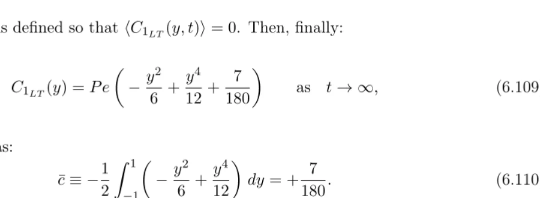
32

3.5.3

Finalizing the Second Moment Solution

. . . .

40

CHAPTER 4: HIGHER MOMENTS, SKEWNESS, AND KURTOSIS . . . .

41

4.1

The Third Moment Solution . . . .

41

4.2

Skewness

. . . .

43

4.3

Fourth Moment . . . .

43

4.4

Kurtosis . . . .

45

CHAPTER 5: MOMENTS IN THE CIRCULAR PIPE GEOMETRY . . . .

46

5.1

Circular Pipe Geometry . . . .

46

5.2

Moments Expansion Method in the Circular Pipe Geometry . . . .

47

5.2.1

First Moment . . . .

48

5.2.2

Second Moment . . . .

50

5.2.3

Third Moment . . . .

51

5.3

Full Skewness . . . .

52

CHAPTER 6: ASYMPTOTICS FOR THE MOMENTS SOLUTIONS

. . . .

53

6.1

Generalized Short-time Asymptotic . . . .

53

6.1.1

First Moment . . . .

53

6.1.2

Higher Moments . . . .

54

6.2

Short-time Asymptotics in the Parallel Plates Geometry . . . .

56

6.2.1

First Moment . . . .

56

6.2.2

Second Moment . . . .

59

6.2.3

Third Moment . . . .

64

6.2.4

Short-Time Asymptotics for Full Moments, Skewness, and Kurtosis . . . .

69

6.3

Short-time Asymptotics in the Circular Pipe Geometry . . . .

70

6.3.1

Exact Moments Asymptotics . . . .

71

6.4

Long-time Asymptotics for the Infinite Parallel Plates Geometry

. . . .

72

6.4.1

First Moment . . . .

72

6.4.2

Second Moment . . . .

73

6.4.3

Third Moment . . . .

76

6.5

Large Péclet Asymptotics in the Circular Pipe Geometry . . . .

79

CHAPTER 7: SYMMETRIC INITIAL CONDITIONS OF FINITE THICKNESS 81

7.1

Infinite Parallel Plates Geometry . . . .

81

7.1.1

First Moment . . . .

82

7.1.2

Second Moment . . . .

82

7.1.3

Third Moment . . . .

83

7.1.4

Skewness

. . . .

84

7.1.5

Plug Initial Condition . . . .

85

7.2

Circular Pipe Geometry . . . .

86

7.2.1

First Moment . . . .

86

7.2.2

Second Moment . . . .

87

7.2.3

Third Moment . . . .

87

7.2.4

Full Skewness . . . .

88

7.2.5

Plug Initial Condition . . . .

89

CHAPTER 8: HOMOGENIZATION THEORY . . . .

90

8.1

Homogenization in the Infinite Parallel Plates Geometry . . . .

91

8.1.1

Collecting Terms by Powers of

ε

. . . .

93

8.2

Expansion for the Cross-Sectionally Averaged Concentration Evolution . . . 102

8.2.1

Aris’ Moments Hierarchy

. . . 104

CHAPTER 9: HOMOGENIZATION THEORY: ELLIPTICAL GEOMETRIES . 106

9.1

Homogenization in Elliptical Geometries . . . 107

9.1.1

Collecting Terms by Powers of

ε

. . . 110

9.2

Expansion for the Cross-Sectionally Averaged Concentration Evolution . . . 121

CHAPTER 10: EXPERIMENTAL WORK . . . 125

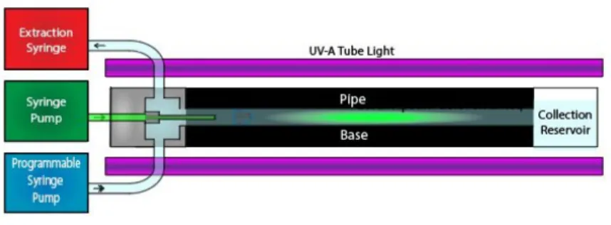
10.1 Relevance for Microfluidics Applications . . . 125

10.2 Experimental Setup and Protocol . . . 127

10.2.1 Brief Description of the Protocol . . . 128

10.2.2 Common Issues with the Protocol

. . . 129

10.2.3 Recent Improvements to the Setup and Protocol

. . . 130

10.3 Rectangular Ducts Experiments . . . 131

CHAPTER 11: EXPERIMENTAL WORK ON TRIANGULAR PIPES

. . . 134

11.1 Experimental Setup for Triangular Pipes . . . 134

11.1.1 Changes in the Setup . . . 135

11.2 Experimental Protocol for the Triangular Pipe . . . 138

11.3 Data Analysis . . . 139

11.3.1 Matching Results from the Two Cameras

. . . 139

11.4 Comparison with Numerical Simulations . . . 140

11.4.1 Issues with the Equilateral Triangle Pipe Cross-Section . . . 141

11.4.2 Change in the Loading Behavior

. . . 145

APPENDIX A: PEEL-OFF IN THE PARALLEL PLATES GEOMETRY . . . 149

A.1 Back to the

Box

Equations

. . . 149

A.1.1

Solving

h

. . . 149

A.1.2

Solving

h

. . . 150

A.1.3

Solving

h

. . . 151

A.2 Solving the Problems Due to Boundary Conditions Evolution . . . 153

A.2.1

Solving

V

. . . 153

A.2.2

Solving

W

. . . 154

A.3 Building the Final

C

Solution

. . . 164

APPENDIX B: HOMOGENIZATION: PARALLEL PLATES GEOMETRY . . . 166

APPENDIX D: HOMOGENIZATION: ELLIPTICAL GEOMETRIES . . . 168

APPENDIX E: EXPERIMENTS ON RECTANGULAR PIPES

. . . 170

E.1 Materials

. . . 170

E.2 Protocol . . . 170

E.3 MATLAB Codes . . . 176

APPENDIX F: EXPERIMENTS ON TRIANGULAR PIPES . . . 185

F.1 Materials

. . . 185

F.2 MATLAB Codes . . . 185

LIST OF FIGURES

2.1

Visualization of Poiseuille flow. . . .

7

2.2

Section of the tube considered by G.I. Taylor [1]. . . .

8

2.3

Schematic of Sir G.I. Taylor’s experimental setup from [1]. . . .

13

2.4

Comparison of experimental and theoretical results from [1]. . . .

15

2.5

Typical distributions shapes and relative loading. . . .

18

2.6

Aris’s pipe system [8]. . . .

19

3.1

Diagram of the infinite parallel plates reference system. . . .

23

3.2

Visualization of the solute initial condition. . . .

25

3.3

Domain

u

in the residue theorem [3]. . . .

38

4.1

Plot of the skewness analytical solutions. . . .

44

4.2

Comparison of analytical solutions to Monte Carlo simulations. . . .

45

5.1

Diagram of the infinite circular pipe geometry. . . .

46

6.1

Long time asymptotic for the first moment in the infinite parallel plates domain.

. .

73

9.1

Elliptical pipe schematic. . . 107

10.1 Schematic of the improved experimental setup. . . 127

10.2 Sample of images produced by MATLAB when analyzing the data. . . 129

10.3 Schematic of rectangular duct of aspect ratio

λ. . . 131

10.4 Three stages in the experimental run for the thin rectangular duct geometry.

. . . . 132

10.5 Comparison between experiments and Monte Carlo simulations. . . 133

11.1 Picture of the current experimental setup. . . 135

11.2 Picture of the experimental setup during an experimental run. . . 136

11.3 Triangular pipe orientation with respect to the camera lenses. . . 137

11.4 Apothem of an equilateral triangle rotated

270

counterclockwise. . . 138

11.7 Overlap of the initial condition curves from experiment and Monte Carlo simulation. 141

11.8 Pictures of pipe cross-sections for various geometries taken with a micro lens. . . 142

11.9 Picture of the equilateral triangle pipe cross-section taken with a micro lens. . . 142

11.10 Images showcasing issues with the triangle cross-section.

. . . 143

11.11 Comparison of experiments and Monte Carlo simulations. . . 144

11.12 Comparison of experiments and Monte Carlo simulations for

a

= 0.0768

cm. . . 145

11.13 Skewness evolution in time [4, 7].

. . . 146

11.14 Skewness evolution in time for pipe of equilateral triangle cross-section. . . 147

11.15 Comparison of experiments and Monte Carlo simulations at slow flow rate. . . 148

LIST OF TABLES

CHAPTER 1

Introduction

The first discoveries of interest describing the behavior in time of a passive solute flowing slowly

through a pipe were made by the British fluid dynamicist Sir G.I. Taylor in 1953 [1].

Taylor

Dispersion

is the theory explaining the evolution in time of the concentration of a passive tracer

injected into a fluid flowing slowly through a straight pipe. Taylor’s result demonstrated theoretically

and experimentally how the interaction between fluid advection and diffusion boosts the spreading

of the solute. This enhanced diffusivity is proportional to

(r U)

/κ, where

r

is the pipe radius,

U

is the characteristic speed of the fluid flow, and

κ

is the molecular diffusion coefficient. While at

very short- and long-times with respect to the

diffusion time

,

t

∝

r

/κ, the solute concentration is

asymptotically Gaussian, Taylor observed that at intermediate times the symmetry is broken and

the solute behavior is highly non-Gaussian.

In 1956 Robert Aris introduced a new approach to study the tracer evolution modeled by the

advection-diffusion equation. The so-called

Moments Expansion Method

allows for the tracer behavior

to be described through its longitudinal moments (along the pipe length) which satisfy a hierarchy

of driven advection-diffusion equations [8].

Utilizing this approach, Aris and others have derived both exact and asymptotic solutions for the

infinite parallel plates geometry and the circular pipe geometry [8, 9, 10]. This same problem has

also been investigated with an homogenization theory approach for the same geometries for arbitrary

point sources [11, 12].

In the past decades, new

lab-on-chip

technologies have been developed with the potential of

reducing cost and increasing efficacy for experimental protocols in a variety of microfluidics systems,

spanning from engineering to medical applications. An interesting aspect of these new manufacturing

techniques is that the microchannels can be easily etched

ad hoc

, with control over their cross-section.

attempted to address this by studying its effects on Taylor’s effective diffusivity [13, 14, 15, 16, 17].

Nonetheless, the effect of the fluid flow on the symmetry-breaking in the concentration profile is still

largely unexplored.

In particular, the tracer concentration curve breaks symmetry in opposite ways in the infinite

parallel plates and circular pipe cases. While this result was first derived asymptotically [12], it has

been confirmed by results reported in this dissertation and served as original motivation for this

work. Single-series solutions for exact and cross-sectionally averaged longitudinal moments in the

circular pipe and infinite parallel plates geometries are reported here and have been published in

2015 [2].

These newly obtained formulae showcased how even with mathematically similar flows, the

symmetry breaks in opposite ways in those two geometries; the cross-sectionally averaged skewness

(the centered, normalized third moment) for the concentration is positive in the case of the circular

pipe, and negative in the case of the infinite parallel plates. Based on these first results, we included

other classes of cross-sections, hoping to connect the positive skewness reported in the circular pipe

case to the negative skewness of the infinite parallel plates.

We considered the family of pipes of elliptical and rectangular cross-sections, deriving short-time

asymptotic results for the longitudinal moments valid for any cross-sectional geometry [2]. This

highlighted how the short-time skewness is zero for all ellipses and sign-definite for all rectangles,

allowing us to identify a cross-over aspect ratio separating rectangles with negative and positive

skewness [2].

Extending the work to long-time studies [4, 5] allowed us to pursue experimental investigations,

as short-time results are not observable in a laboratory setting. Long-time asymptotics and numerical

predictions have been experimentally confirmed for rectangular pipes [4, 5, 6]. Both rectangles and

ellipses have sign-indefinite skewness at long-time, separated by a geometry of incredibly similar

aspect ratio [4, 5].

We also approached this problem via homogenization theory, hoping to obtain a description

of the entire concentration evolution rather than just its longitudinal moments. This method was

applied to the infinite parallel plates first, and then extended to elliptical pipes. Homogenization

results have been compared to Monte Carlo simulations.

we have extended our experimental investigation to include pipes of equilateral triangle cross-section.

Equilateral triangles are the only regular polygon cross-section for which the loading behavior of the

concentration curve switches in time, from back-loaded (positive skewness) to front-loaded (negative

skewness) [4, 7]. Motivated by this interesting behavior, we have worked on experiments with long

triangular pipes to observe this sign-change in the cross-sectionally averaged skewness.

CHAPTER 2

Theoretical Background

When a passive solute is injected in a straight pipe with laminar steady flow, the tracer evolves

undergoing an advection-diffusion process. In particular, we are interested in studying how the

concentration profile of the solute changes in time.

2.1

The Advection-Diffusion Equation

The advection-diffusion equation describes phenomena in which particles, energy or other physical

quantities are transferred throughout a physical system via diffusion and transport. As mentioned,

the equations of motion for a system in which a

passive scalar

is injected in a fluid flow, include the

advection-diffusion equation. With passive scalar or passive tracer we indicate a solute that when

injected in a background flow doesn’t influence its dynamics.

In its non-conservative form, the advection-diffusion equation can be written as:

∂C

∂t

=

∇ ·

(κ

∇C)

− ∇ ·

(¯

u C) +

R,

(2.1)

where

C

is the passive scalar concentration,

κ

is the diffusion coefficient

,

u

¯

is the average fluid

velocity, and

R

describes the sources or sinks of the quantity of interest. In our system of interest,

the diffusion coefficient is constant with respect to the spatial coordinates

(x, y, z), there aren’t any

sources or sinks (R

= 0), and the velocity field describes an incompressible flow (i.e. it has null

divergence,

∇ ·

u

¯

= 0) [18, Chapter 2]. Therefore, equation (2.1) simplifies to:

∂C

∂t

=

κ

∇

2

_C

₋

_u

_¯

_{· ∇C.}

_(2.2)

1_{Thediffusion coefficientordiffusivityκ(with SI unit[m}2_{/s]) is the proportionality constant between the diffusive}

In this form, the advection-diffusion equation combines aspects of both parabolic and hyperbolic

second order partial differential equations

.

The advection-diffusion equation can be derived from the

continuity equation

, which expresses in

local form the

conservation law

of a physical quantity using the flux of such quantity through a

closed surface. The differential form of the continuity equation is:

∂C

∂t

+

∇ ·

~j

=

s,

(2.4)

where

~j

is the total concentration flux and

s

is the net volumetric source, in our system

s

= 0. In a

system described by the advection-diffusion equation, there are two sources of flux:

- the diffusive flux for which an expression can be obtained by the approximation of

Fick’s first

law

:

~j

=

−κ

∇C,

(2.5)

where

~j

is the diffusive flux, measuring the amount of substance flowing through a small

area during a small time interval.

- the advective flux for which an expression is given by:

~j

= ¯

u C.

(2.6)

2_{In general, a second order partial differential equation:}

Autt+Butx+Cuxx+Dut+Eux+F= 0, (2.3) - is parabolic ifB2_{−4AC= 0(e.g. the heat equationw}

t−k∇2w= 0, wherek is a constant); - is hyperbolic ifB2−4AC >0(e.g. the wave equationwtt−k2∇2w= 0, wherek is a constant).

3

Conservation lawsin physics state that a particular measurable property of an isolated physical system does not change as the system evolves. Conservation laws exist for mass, momentum, energy and other physical quantities. We will take advantage of conservation laws for our system when deriving short time asymptotic solutions for the longitudinal moments in arbitrary geometries (see section 6.1).

4_{Fick’s first law connects the diffusive flux with the concentration, assuming the surrounding fluid in the system to be}

In a steady-state system such as ours, the total flux is given by the sum of the two flux sources:

~j

=

~j

+

~j

=

−κ

∇C

+ ¯

u C,

(2.7)

giving the following form for the continuity equation (2.4):

∂C

∂t

+

∇·

−

κ

∇C

+ ¯

u C

= 0

.

(2.8)

Assuming the diffusion coefficient

κ

to be constant (as in equation (2.2), it is possible to swap the

order of the derivatives to obtain:

∇ ·

(κ

∇C) =

κ

(∇ · ∇)C

=

κ

∇

_{C ,}

_(2.9)

finally giving the same expression for the advection-diffusion equation as in equation (2.1).

2.2

Taylor Dispersion

The boost in solute dispersion due to the interplay between advection and diffusion is an effect

named

Taylor dispersion

after the British fluid dynamicist Sir G.I. Taylor, whose work has laid the

foundations for this research (cf. [1], [20]).

The laminar shear background flow smears out the concentration profile in the direction of the

flow while increasing the rate at which it spreads in that direction. In 1953, G.I. Taylor observed

the way in which salts are dispersed along a tube with uniform background

Poiseuille flow

[1]. Since

dispersion in such a steady flow is due to the combined action of advection parallel to the axis of the

pipe and molecular diffusion in the radial direction, in order to describe the phenomenon dispersion

by advection alone will be considered at first, and then the effect of molecular diffusion will be

introduced.

2.2.1

Poiseuille Flow

figure 2.1. The fluid motion happens through the sliding of such infinitesimal lamina one over the

other without any kind of reshuffling of the fluid, not even at a microscopic level.

Figure 2.1: Visualization of Poiseuille flow. a) A cylindrical tube showing the imaginary concentrical

lamina. b) A longitudinal cross-section of the tube showing the lamina moving at different speeds.

Those closest to the tube boundary are moving slower while the ones near the center are moving

faster.

The flow is constant in time and it is determined by the viscous forces. The Poiseuille equation

can be written as:

∆p

=

8

µ L Q

π a

,

(2.10)

where

∆p

identifies the pressure drop,

µ

is the dynamic viscosity

,

L

is the characteristic length of

the pipe,

Q

represents the volumetric flow rate, and

a

is the radius of the pipe [22]. Such equation is

based on the the following assumptions:

- the fluid must be viscous and incompressible;

- the flow must be laminar;

- the pipe must have a constant circular cross-section and needs to be substantially longer than

its diameter;

5_{When two layers of liquid in contact with each other move at different speeds, there is a shear force between them.}

Such a force is proportional to the area of contactA, the velocity gradient in the direction of flow∆vx/∆yand a proportionality constantµcalleddynamic viscosity[21]. The shear forceF is given by:

F =−µ A∆vx

∆y, (2.11)

- there must be no acceleration of fluid in the pipe.

A flow that satisfies such conditions and for which the Poiseuille equation is valid is called a

Poiseuille

flow

.

According to experimental observations of a solution injected into a tube through which water

is flowing, the region in which the solution is concentrated moves downstream. Since the stream

velocity varies over the cross-section of the pipe, the part of injected material initially positioned near

the centre of the tube will be advected faster than the parts positioned near the walls, determining a

parabolic velocity profile.

2.2.2

Dispersion by Advection Alone

Following the reasoning of Sir G.I. Taylor [1], in a circular pipe of radius

a

the flow velocity

u

at

distance

r

from the centered longitudinal axis is given by:

u

=

u

1

−

r

2

a

,

(2.12)

where

u

is the maximum velocity at the axis, as shown in figure 2.2. If at time

t

= 0

the solute is

distributed symmetrically in the cross-section, so that the concentration is

C

=

C(x, r), after time

t

has passed the concentration

C

will be given by:

C

=

C(x

−

u t, r).

(2.13)

Figure 2.2: Section of the tube considered by G.I. Taylor [1], where

x

is the longitudinal flow-wise

axis,

a

is the radius, and

r

represents the radial distance from the center.

6

2.2.3

Effect of Molecular Diffusion on Solute Dispersion

Assuming that the concentration is symmetric about the central longitudinal axis of the pipe (so

that

C

is a function of

r,

x, and

t

only), the diffusion equation (2.1) can be written as:

κ

∂

C

∂r

+

1

r

∂C

∂r

+

∂

C

∂x

=

∂C

∂t

+

u

1

−

r

2

a

∂C

∂x

,

(2.14)

where the coefficient of molecular diffusion

κ

is assumed to be independent of the solute concentration

.

Given the geometric characteristics of the system (as shown in figure 2.2), the Laplacian operator in

the equation is written in polar coordinates (with

C

depending on

r,

x, and

t

only). Finally, it is

assumed that the contribution of the second derivative in the longitudinal direction is much less

than that in the radial direction

_.

Writing

ρ

=

r/a, equation (2.14) becomes:

∂

C

∂ρ

+

1

ρ

∂C

∂ρ

=

a

κ

∂C

∂t

+

a

u

κ

(1

−

ρ

2

₎

∂C

∂x

,

(2.16)

and the boundary condition representing the impermeable wall is given by:

∂C

∂ρ

= 0

at

ρ

= 1.

(2.17)

Even when knowing the distribution of the concentration

C

at

t

= 0

(i.e. the initial condition for

the problem), it is still very difficult to find an analytic solution valid for all values of

ρ,

x, and

t.

However, approximate solutions can be computed as long as the following limiting conditions are

satisfied:

(A) the changes in the concentration due to advective transport along the tube take place in such

a short time that the effect of molecular diffusion can be neglected;

7

When soluble salts are used, the last assumption is not strictly accurate, but the error introduced is very small and such an assumption is necessary for the solution of the problem.

8_{That is:}

∂2_C

∂x2

∂2_C

∂r2 +

1 r

∂C

(B) the time necessary for advective transport to produce noticeable effects is long if compared to

the

time of decay

, during which radial variations of concentration are reduced to a fraction of

their initial value due to the action of molecular diffusion.

To find the conditions of validity for (B), it is necessary to calculate how fast the concentration

(varying with

r) degenerates into a concentration that is uniform in the cross-section. Solutions to

equation (2.16) for which

= 0, and the variables

ρ

and

t

are separated, are of the form:

C

=

e

J

(a ρ α

1

2

κ

1

2

),

_(2.18)

where

J

is the zeroth order Bessel function of the first kind. The boundary condition in (2.17)

assures

= 0, that is:

J

(a α

1

2

κ

1

2

) = 0.

(2.19)

The root of (2.19), corresponding to the lowest possible value of

α, is given by:

a α

κ

2

≈

3.8,

(2.20)

so that the time necessary for the radial variation of

C

from equation (2.18) to diminish to

1/e

of its

initial value is given by:

t

=

a

3.8

_κ

,

(2.21)

called

Taylor time

or

diffusion time

. If the dispersing material is spread over a length of tube of

order

L, the time necessary for advective transport to induce an observable change in

C

is of order

L/u

. Therefore, in order for condition (B) to be valid, it must be true that:

L

u

a

2

3.8

_κ

.

(2.22)

2.2.4

Effect of Using Condition (B)

Since molecular diffusion along the longitudinal axis has been neglected based on condition (A),

the transfer of solute in the longitudinal direction is assumed to be due to advection only.

Letting:

x

=

x

−

1

2

u

t,

(2.23)

equation (2.16) becomes:

∂

C

∂ρ

+

1

ρ

∂C

∂ρ

=

a

κ

∂C

∂t

+

a

u

κ

1

2

−

ρ

2

∂C

∂x

.

(2.24)

Since for

x

to be constant the mean velocity across planes must be zero, the transfer of solution

across these planes depends only on the radial variation of

C.

If the concentration were independent of

x

and condition (B) were satisfied, then any radial

variation in

C

would disappear quickly. Therefore, small radial variations in the concentration can

be calculated from:

∂

C

∂ρ

+

1

ρ

∂C

∂ρ

=

a

u

κ

1

2

−

ρ

2

∂C

∂x

,

(2.25)

where

1

can be taken as independent of

ρ. A solution to this equation that satisfies the boundary

condition (2.17) is given by:

C

=

C

+

A

ρ

−

1

2

ρ

4

,

(2.26)

where

Cx

is the value of

C

at

ρ

= 0

and

A

is a constant calculated substituting solution (2.26) in

equation (2.25):

A

=

a

2

_u

8κ

∂C

∂x

.

(2.27)

The rate of transfer

Q

of the concentration across the section at

x

is given by:

Q

=

−2πa

Z

0

u

1

2

−

ρ

2

C ρ dρ.

(2.28)

Substituting the expression for

C

(containing

A) in equation (2.28), we obtain:

Q

=

−

π a

4

_u

192

κ

∂Cx

∂x

.

(2.29)

the concentration over a cross-section of the tube

, it can be written:

∂C

∂x

=

∂C

∂x

,

(2.31)

so that the expression for the rate of transfer

Q

becomes:

Q

=

−

π a

4

_u

192

κ

∂C

∂x

.

(2.32)

Therefore,

C

is dispersed relative to a plane moving with velocity

u

, exactly as if its diffusion

was induced by a process responding to the same laws of molecular diffusion but with an

effective

diffusion coefficient

κe

[1]. For a straight circular pipe, this term is of the form:

κ

=

a

u

192

κ

.

(2.33)

Through the continuity equation for

Cm

, it can be shown that no material is lost in the process.

Specifically, taking the time derivative at a point where

x

is constant:

∂Q

∂x

=

−

π a

∂C

∂t

.

(2.34)

Substituting

Q

above, the equation governing longitudinal dispersion can be written as:

∂C

∂t

−

κ

∂

C

∂x

= 0.

(2.35)

2.2.5

Experimental Procedures

With the aim of finding

Cm

as a function of

x

at a fixed time, Sir G.I. Taylor used a colorimetric

method hoping for results without disturbing the fluid motion [1].

9

In the experiments described by Sir G.I. Taylor [1], the mean value of the concentration over a cross-section of the tubeCmis measured for different experimental conditions. In general,Cmis defined as:

Cm= 2 a2

Z a

0

To satisfy condition (B), he used a tube of small bore with an internal diameter

a

≈

0.05

cm

and

a length

L

= 152

cm. His solute was a solution of potassium permanganate (K M n O

) characterized

by a transparent dark purple coloring

. The initial concentration of the solution was set to

1%

of

K M n O

and

99%

of slightly acidulated water. Numerous solutions of known concentrations were

then made mixing the

1%

solution with various proportions of distilled water.

As shown in figure 2.3, a comparison tube was placed in a light frame sliding along the main

pipe, in order to find the position where the colors of the two pipes are identical

_{. At this location,}

the concentration could be determined as a function of

x. This method had the advantage that

comparisons were made only between colors whose spectrum and intensity were both identical at

the determined position.

Figure 2.3: Schematic of Sir G.I. Taylor’s experimental setup from [1].

A

identifies the pipe and

B

the comparison tube;

C

is a ground-glass plate illuminated as uniformly as possible and

D

is a line

ruled on

C.

To make a measurement, the comparison tube (B) was filled with a solution of known

concen-tration and moved until the color intensity was about the same as that in the main pipe (A) close

to its mid-point. Then, the ground-glass plate (C) was moved until the line (D) crossed the two

tubes (A

and

B) at the point where their colors were identical. Finally, the distance

x

of the line

(D) from the entry end of the main pipe was measured.

10_{When seen in a bottle, potassium permanganate is so dark that it almost looks black, but in a pipe with such a}

small bore the coloring gets to a dark shade of purple.

11

Sir G.I. Taylor first proved that for a time inferior to diffusion time molecular diffusion didn’t

interfere with advection. Then, moved on to a set of experiments in which the time of the flow was

set to be long compared to the diffusion time. These experiments were done introducing a small

volume of concentrated solution of mass

M

and bringing the point

x

=

u

t

to

110

cm.

From a theoretical point of view, the space between two ideal planes positioned at

x

= 0

and

x

=

X

(where

X/a

is small), was considered to be filled initially with a concentration

C

of

solute. The amount of solute lying between

r

and

r

+

δr

is constant during the flow and equal to:

2

π r C

X δr, from equation (2.13). Then, the solute is assumed to become distorted in time into a

paraboloid:

x

=

u

t

1

−

r

2

a

.

(2.36)

The total amount of solute between

x

and

x

+

δx

can be calculated as:

2

π r C

X δx

(dr/dx). Since

r

(dr/dx) =

−(a

_u

0

t)/2, then:

C

=

1

π a

_δx

(2

π C

X δx)

a

2

u

t

=

C

X

u

t

.

(2.37)

Hence,

C

can be written as:

Cm

=

u0t

for

0

< x < u

t,

(2.38)

Cm

= 0

for

x <

0

and

x > u

t.

(2.39)

Therefore, in this case the solution to equation (2.35) expressing the evolution of longitudinal

dispersion, is:

C(x, t) =

M

exp

−

4κet

√

4

a

_π

_κ

e

t

.

(2.40)

One of the most remarkable predictions of this analysis is the fact that an initially concentrated

mass

M

would be dispersed symmetrically about the point

x

=

u

t

in spite of the great asymmetry

of the velocity field over the cross-section

. In fact, past diffusion time it was observed that the

12

This return to symmetry is observed at long-time, past the diffusion time; this is why a sufficiently long value forx

distribution of the solute concentration about

x

was very symmetrical, as shown in figure 2.4. To

compare the experimental results with the theoretical prediction of equation (2.40), the error curve

of expression:

C

= 0.0041

exp

−

(x

−

110)

2

121

,

(2.41)

was added in figure 2.4; here the constants were chosen such that the curve would fit as well as

possible the experimental data [1].

Figure 2.4: Comparison of experimental and theoretical results from [1]. The empty circles

◦

are

theoretical predictions (as expressed in equation (2.41)), while the filled circles

•

represent the

experimental data. Measuring time: 11 minutes.

2.3

Aris’ Generalization of Taylor’s Coefficient

In his work dated 1956 [8], R. Aris presented a generalization of the effective diffusion coefficient

κ

previously obtained by G.I. Taylor [1], valid without any restriction on the distribution of solute

.

Aris’

enhanced diffusion coefficient

K

can be written as:

K

=

κ

+

c

a

2

_u

_¯

κ

,

(2.42)

where

κ

is the molecular diffusion coefficient of the solute,

a

is the characteristic cross-sectional

dimension of the tube,

u

¯

is the mean flow velocity, and

c

is a computable factor depending on the

13

tube cross-sectional geometry

. For a tube of circular cross-section

c

= 1/48, giving:

K

=

κ

+

a

2

_u

_¯

48

κ

,

(2.44)

which is the sum of the molecular diffusion coefficient

κ

and the effective diffusion coefficient

κ

, as

introduced by G.I. Taylor

[1].

This last expression for

K

can also be written in terms of the

Péclet number

P e

as:

K

=

κ

1 +

P e

2

48

,

(2.45)

which is valid if

P e

L/a, where

L

and

a

are the characteristic longitudinal and cross-sectional

dimensions of the pipe, respectively [8].

2.3.1

The Péclet Number

The

Péclet number

is a dimensionless parameter used in the study of transport phenomena in

fluid flows. It relates the importance of advective to diffusive effects on a certain physical quantity.

In the context of mass dispersion, the Péclet number is defined as the product of the

Reynolds

14

The constantc is a pure number depending on the geometry of the cross-section and on functionsχandψ (cf. section 2.5). It can be expressed as:

κ=χ ψ, (2.43)

whereχdefines the flow velocity relative to the mean andψrepresents the variation of the diffusion coefficient. For a circular cross-sectionψ= 1.

15

number

and the

Schmidt number

:

P e

=

a

u

¯

κ

=

Re

·

Sc,

(2.48)

where

a

is the characteristic cross-sectional length of the geometry,

u

¯

is the mean fluid velocity, and

κ

is the molecular diffusion coefficient [24].

2.4

The Moments Expansion Method

The phenomenon of Taylor dispersion introduced the concept of effective diffusion coefficient

(equation 2.33) when analyzing the dispersion of a soluble matter in a fluid flowing through a straight

tube of circular cross-section (cf. [1, 20]).

The first step in generalizing such a result was made by R. Aris in 1956 by removing the

restrictions on the flow applied by Taylor [8]. As reported in section 2.3, Aris was able to write a

generalized expression for the enhanced diffusion coefficient

K

starting from Taylor’s work valid for

tubes of any cross-sectional geometry. In order to obtain such result, Aris focused on the spatial and

temporal evolution of the centre of gravity of the solute concentration and its higher longitudinal

moments.

Specifically, the

moments expansion method

introduced by Aris [8] is the first analytical approach

we have used in this work. Therefore, it will be discussed at length in the following sections.

16

TheReynolds numberReis a dimensionless parameter used in fluid mechanics to measure the ratio of inertial forces to viscous forces. For the flow in a pipe, the Reynolds number is defined as:

Re= u a¯

ν , (2.46)

whereu¯is the mean fluid velocity[¯u] =m/s,ais the characteristic cross-sectional length[a] =m, andν is the kinematic viscosity[ν] =m2_{/s[23]. The Reynolds number is used to characterize flow regimes: at low Reynolds,}

viscous forces are dominant and laminar flow occurs characterized by a smooth, constant fluid motion; at high Reynolds, inertial forces are dominant and turbulent flow occurs characterized by chaotic eddies, vortices, and other flow instabilities. The work reported in this thesis is in the laminar regime at low Reynolds numbers, i.e.Re∼1.

17_{TheSchmidt numberis a dimensionless parameter relating the importance of viscous to diffusion effects for a physical}

quantity. It is defined as:

Sc= ν

κ, (2.47)

2.4.1

Longitudinal Moments

The

n

longitudinal moment of a real-valued probability density function (pdf)

f

(x), of a

real-valued random variable

x, about a value

x

, is given by:

f

=

Z

−∞

(x

−

x

)

f

(x)

dx.

(2.49)

Knowing all the moments of

f(x)

gives a complete description of the pdf. The moments about

the mean

µ

of the pdf (x

=

µ) are called

central moments

and describe the shape of the function

independently of translation.

The most commonly used moments are the

mean

µ

of the distribution (first (raw) moment of

x),

the

variance

σ

(second central moment) measuring the "width" of the distribution with respect to

the mean [25], the

skewness

(third central moment) measuring the "asymmetry" of the distribution

with respect to the mean, and the

kurtosis

(fourth central moment) measuring the "tailedness" of

the distribution [26].

2.4.2

Skewness

As mentioned, the

skewness

of a distribution is a measure of its asymmetry with respect to the

mean. Skewness is the third central moment and it is defined to be a non-dimensional quantity

.

Figure 2.5: Front-loaded distribution with negative skewness (left); back-loaded distribution with

positive skewness (right) [2].

A distribution with negative skewness (shown in figure 2.5, left) is typically

front-loaded

, presenting

the peak in the front followed by a tapering tail; for a front-loaded distribution the mean is to the left

18

of the median

[7]. A distribution with positive skewness (figure 2.5, right) is typically

back-loaded

,

presenting a slow build-up with a peak in the back; for a back-loaded distribution the mean is to the

right of the median [7].

The skewness of a pdf of a continuous variable

x, is given by:

Sk

=

E

[(x

−

µ)

3

_]

(

E

[(x

−

µ)

_])

,

(2.50)

where

µ

is the mean of the distribution and

E

[·]

is the expectation operator

.

2.5

Moments Expansion of the Concentration

Following Aris’ line of thinking, we derive the equations to be solved for the moments of the

solute concentration.

Figure 2.6: Aris’s pipe system: infinite straight circular tube with longitudinal x-axis.

Ω

is the

cross-sectional domain in the

yz-plane (the cross-section of the tube).

When considering an infinite tube (as shown in figure 2.6) with a steady uniform fluid flow, the

direction of the flow velocity

u

is oriented as the longitudinal x-axis at any point inside the tube,

and is a function of both cross-sectional dimensions

y

and

z:

u(y, z

) = ¯

u

(1 +

χ(y, z)),

(2.51)

where

u

¯

is the mean velocity and

χ(x, y)

defines the velocity relative to the mean. In case of a

19

Themedianof distribution separates the mass of the distribution in half; that is, half of the mass will be to the left of the median, and half to the right at all times.

20

The expectation operator is a linear operator used to express the statistical mean of a random variablex. In casex

no-slip condition

at the wall

, on the perimeter

∂Ω

of the domain

χ

=

−1. The concentration of

solute at a point

(x

, y

, z

)

and time

t

in the tube is indicated as

C(x

, y

, z

, t

)

and

κ ψ(y, z)

represents its diffusion coefficient

.

As introduced earlier on, the equation describing the evolution of the concentration

C

is a form

of the advection-diffusion equation (cf. equation 2.2) given by:

1

κ

∂C

∂t

=

∇(ψ

∇C)

−

¯

u

κ

(1 +

χ)

∂C

∂x

.

(2.52)

In order to make the calculations easier, it can be useful to consider a reference frame moving

with the mean speed of the stream and reduce the variables to non-dimensional form. Therefore, we

apply the following change of variables:

ξ

=

x

−

u t

¯

a

,

η

=

y

a

,

ζ

=

z

a

,

τ

=

κ

a

t,

µ

=

a

κ

u,

¯

(2.53)

where

a

is the characteristic dimension of the cross-section

Ω. Then, the concentration problem

becomes:

∂C

∂τ

=

ψ

∂

C

∂ξ

−

µ χ

∂C

∂ξ

+

∂

∂η

ψ

∂C

∂η

+

∂

∂ζ

ψ

∂C

∂ζ

,

(2.54)

together with the following initial and boundary conditions:

C(ξ, η, ζ,

0)

=

C

(ξ, η, ζ),

(2.55)

ψ

∂C

∂ν

=

0

on

Ω,

(2.56)

where

∂/∂ν

indicates differentiation along the direction normal to

Ω.

The nth longitudinal moment of the distribution of solute through the cross-section (η, ζ

) at time

τ

is given by:

cn(η, ζ, τ

) =

Z

−∞

ξ

C(ξ, η, ζ, τ

)

dξ,

(2.57)

21

Ano-slip boundary conditionsets the velocity of the fluid relative to the wall as zero.

22_{The functionψ(y, z)defines the variation of the diffusion coefficient andκis its mean value over the cross-section of}

the tube.

and the nth moment of the cross-sectionally averaged distribution of solute in the tube is:

mn(τ

) =

h

cn

i

=

1

|Ω|

Z

Ω

cn

dη dζ,

(2.58)

where the

h · i

operator indicates averaging over

Ω.

The condition to be imposed on the concentration

C

as

ξ

→ ±∞

is that both of these moments

(cn

and

mn

) exist and are finite. Such a condition is satisfied if the solute is initially contained in a

finite length of tube.

Multiplying equation (2.54) by

ξ

and integrating with respect to

ξ

in

(−∞

,

∞)

gives:

∂c

∂τ

=

∂

∂η

ψ

∂c

∂η

+

∂

∂ζ

ψ

∂c

∂ζ

+

n(n

−

1)ψ c

+

n µ χ c

,

(2.59)

and the two conditions (2.55) and (2.56) become:

c

(η, ζ,

0)

=

c

(η, ζ

),

(2.60)

ψ

∂c

∂ν

=

0

on

Ω.

(2.61)

Using Green’s theorem

and averaging equation (2.59) over the cross-section of

Ω, yields:

d m

dτ

=

n

(n

−

1)h

ψ c

i

+

n µ

h

χ c

i,

(2.63)

and condition (2.60) becomes:

mn(0) =

mn

.

(2.64)

For

n

= 0,

1,

2, . . .

, equation (2.59) bound with conditions (2.60) and (2.61) form a hierarchy

of inhomogeneous problems solvable for the

c

moments. Such systems can be solved for as many

24

Green’s Theorem[27] - LetδS be a simple closed curve in the plane, positively oriented and piecewise smooth.

LetS be the surface bounded by the curveδS. Iffandgare two real-valued functions of real-valued variables with continuous partial derivatives on an open region containingS, then:

Z

δS

(f dx +g dy) = Z Z

S

∂g ∂x−

∂f ∂y

dx dy= I

δS

CHAPTER 3

Exact Moments in the Parallel Plates Geometry

Instead of leading with a more complex three-dimensional system, the first geometry we study is

the infinite parallel plates system.

The aim of this first research step is to solve the moments equations to obtain single-series exact

solutions dependent on the cross-sectional variable as well as time. In previous works (such as [12]),

expressions for the first two moments have been calculated numerically or in their cross-sectionally

averaged version. A new approach to analytically solve the problem was introduced for this work;

we have named

Peel-Off Method

.

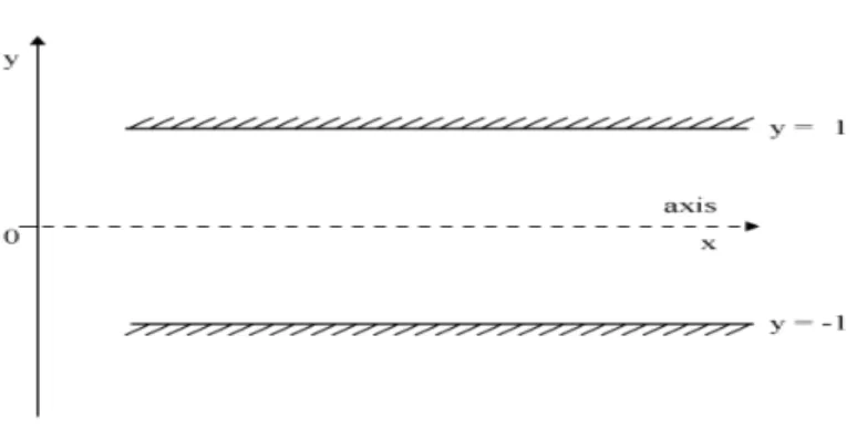
3.1

Problem Setup

The infinite parallel plates geometry is shown in figure 3.1. The longitudinal

x-axis of the

coordinate system is set equidistant from the plates, so that the plates are postioned at

y

=

−1

and

y

= 1

along the

y-axis.

Figure 3.1: Diagram of the infinite parallel plates reference system.

at specific instants in time.

The solute chosen is a passive tracer, that is, it is made of non-reactive and non-interactive

particles. It is subject only to molecular diffusion and advection, but it does not influence the

dynamics of the background flow.

The flow

u(y)

˜

is a laminar steady-state solution to the Naiver-Stokes equations with

no-slip

boundary conditions (no flow at the wall) driven by a negative pressure gradient

∇p

=

px

<

0:

L(˜

u)

=

2px

µ

,

(3.1)

˜

u|

=

0.

(3.2)

Here,

µ

is the dynamic viscosity of the fluid

, and

L(·)

is the Laplacian operator in the infinite

parallel plates geometry:

L(·) =

∂

2

_(·)

∂y

.

(3.3)

The solute evolves in time with a parabolic flow profile; this is true for both the infinite parallel

plates and the circular pipe geometries. The flow solution in physical coordinates is given by:

˜

u(y) =

U

1

−

y

2

a

,

(3.4)

where

a

is the half-distance between the plates,

a

= 1, and

U

is the centerline maximum velocity,

U

=

−

µ

. We mostly work with a mean-zero flow

u, such that

u

= ˜

u−h˜

ui

where the cross-sectional

averaging operator

h · i

is defined as:

h · i

=

1

2

Z

−1

(·)

dy.

(3.5)

The mean-zero flow

u(y)

is:

u(y) =

U

1

3

−

y

a

.

(3.6)

The solute is introduced into the infinite parallel plates as a symmetric, thin, transversally

1

uniform strip centered at

x

= 0. The initial condition for the solute is a delta function in the

longitudinal direction while span-wise uniform; it is expressed as:

C

(y)|

=

δ(x).

(3.7)

Such a form for the initial data, evolves parabolically in time as shown in figure 3.2.

Figure 3.2: The initial condition for the solute (thick blue vertical strip, centered at

x

= 0) is a

delta function in the longitudinal

x

direction, while span-wise uniform. The solute evolves in time

following a parabolic trend.

3.2

The Moments Expansion Method

As previously discussed, the injected passive solute undergoes an advection-diffusion process

expressed by:

∂C

∂t

=

K

L(C)

−

u

· ∇C,

(3.8)

where

u

· ∇C

is the advective term (with

u

the mean-zero fluid flow) and

K

∇

_C

_{is the diffusive}

term, with

K

the Aris’ enhanced diffusion coefficient from equation (2.44).

time through its moments

.

By applying the moments expansion method

, we obtain the hierarchy of recursive equations for

the

n

moments of the solute concentration in the infinite parallel plates case:

∂C

∂t

−

∂

C

∂y

=

n(n

−

1)C

+

P e u(y)

n C

.

(3.10)

The initial conditions for the moments problems (corresponding to equation 2.60) are peculiar to

the choice of initial condition for the solute. Since the solute is injected in the form of a delta function

in

x, we have different initial conditions for the zeroth moment (i.e. the

mass

of the problem) and

the higher moments; that is:

C

(y)|

= 1,

C

(y)

= 0.

(3.11)

The problems have homogeneous Neumann boundary conditions (corresponding to equation 2.61)

written as:

∂C

∂y

= 0.

(3.12)

Our goal is to solve the hierarchy of moments equation (3.10) for increasing values of

n. While for

n

= 0

and

n

= 1

(zeroth and first moment) solving such equation is pretty straightforward, moving

on to

n

= 2

(and higher) brings on several difficulties. In particular, more issues arise when keeping

the dependence on the cross-sectional coordinate

y

and when seeking a solution in a single-series

form.

A few cross-sectionally averaged moments solutions to this same problem are available in the

literature and will be used to match some results of this work as a proof of validity. In particular,

2

In general, higher order moments are subdominant to the first few.

3

Comparing equation (3.10) to equation (2.59) (from [8]), notice that in equation (3.10)P eappears in place ofµ. This is because in the change of variables expressed by equation (2.53),µis defined as the non-dimensional form of the diffusion coefficient:

µ=hu˜ia

κ , (3.9)

a previous work by R. Camassa, Z. Lin, and R.M. McLaughlin [12] was chosen as reference and

guidance.

3.3

The Zeroth Moment

For

n

= 0, the zeroth moment of the concentration

C

represents the

mass

of the problem and

can be immediately calculated.

Plugging

n

= 0

in equation (3.10), we obtain the equation to be solved for

C

:

∂C

∂t

−

∂

_C

0

∂y

= 0,

(3.13)

where the recursion is assumed to start with

Cn

=

Cn

= 0. It can be shown that the mass of

the problem is conserved by integrating equation (3.8):

∂

∂t

Z

−1

dy

Z

−∞

dx C(x, y, t) =

Z

−1

dy

Z

−∞

dx

[K

L(C)(x, y, t)

−

(u

· ∇)C(x, y, t)]

.

(3.14)

This results in:

∂

∂t

C

(t) = 0,

(3.15)

expressing the mass conservation law: the mass of the problem

C

is constant.

The definition for the zeroth moment

C

is given by:

C

(y, t) =

Z

−∞

δ(x)

dx

= 1,

(3.16)

where we recognize the initial condition for the problem, as expressed in equation (3.11). Since

the zeroth moment expresses the mass of the solute, it is unsurprisingly connected to the initial

condition of the problem.

3.4

The First Moment

The first moment of the concentration

C

represents its mean and can be calculated by solving

the moments equation (3.10) for

n

= 1. The first moment equation is:

∂C

∂t

−

∂

_C

1

To simplify the calculations (and the writing) of this work, we define the

box

operator as:

(·)

≡

∂(·)

∂t

−

∂

_(·)

∂y

,

(3.18)

giving the following final expression for the

C

problem:

C

=

P e

1

3

−

y

2

,

(3.19)

∂C

∂y

y=±1

=

0,

(3.20)

C

(y,

0)

=

0.

(3.21)

Equation (3.19) is a linear, parabolic, second order partial differential equation [28]; it describes

how the mean of the solute concentration (its first moment) evolves in our fluid system.

In order to solve the PDE, we can express its driver as a Fourier series in sines and cosines [28].

That is, in this case:

fn

=

Z

−1

P e

1

3

−

y

2

cos (n π y)

dy

=

−P e

4 (−1)

(n π)

,

(3.22)

and for the

n

= 0

coefficient (constant value):

f

=

Z

−1

P e

1

3

−

y

2

dy

= 0.

(3.23)

Then, we pose a solution for

C

of the form:

C

(y, t) =

1

2

a

+

∞

X

n=1

an(t) cos (n π y),

(3.24)

which leads to the associated constant coefficient ordinary differential equations (ODE) for the

a

terms:

˙

a

=

−(n π)

a

+

f

,

(3.25)

˙