FORMATION OF UNDERWATER PLUMES AND VELOCITY VARIATIONS DUE TO ENTRAINMENT IN STRATIFIED
ENVIRONMENTS
Chung-Nan Tzou
A dissertation submitted to the faculty at the University of North Carolina at Chapel Hill in partial fulfillment of the requirements for the degree of Doctor of Philosophy in the Department of
Mathematics in the College of Arts and Sciences.
Chapel Hill 2015
ABSTRACT
Chung-Nan Tzou: Formation of Underwater Plumes and Velocity Variations due to entrainment in stratified environments
(Under the direction of Roberto Camassa)
ACKNOWLEDGMENTS
First, I thank my advisors Roberto Camassa and Richard McLaughlin for their guidance and support. Many useful discussion made me able to make progress on this interesting project along the past few years. I am especially grateful on having the opportunity to work in the fluids lab and present many of our research results in many conferences that expands my view of the scientific world. I would also like to thank all of my other committee members, Professor Jeremy Marzuola, Laura Miller and Brian White as well as Claudia Falcon, Shilpa Khatri, Keith Mertens for several helpful conversations in the theoretical and experimental sides of this work. I am thankful to many faculty members in our department for teaching me many useful mathematical tools, and also to having the opportunity to be a lecturer of many advanced math courses, which enforces me to improve my mathematical skills. All the sta↵ members and all the colleagues studying and working in the math department are making here a pleasant environment to do research, and I am very grateful of that.
I would also like to thank many undergraduate research assistants, Johnny Reis, who actually taught me how to run the experiments, and Steve Harenberg, Dani Vasco, William Schlieper, Matt Chancey, Sian Lewis-Bevan, Kaddu Ssekibakke and Chelsea Smith who assisted me on conducting hundreds of day-long experiments.
TABLE OF CONTENTS
LIST OF FIGURES . . . ix
LIST OF TABLES . . . xiii
CHAPTER 1: INTRODUCTION . . . 1
1.1 Experimental results. . . 2
1.2 Theoretical results. . . 3
1.3 Outline . . . 5
CHAPTER 2: CLASSICAL MORTON, TAYLOR, TURNER MODELS . . . 7
2.1 Derivation of MTT models with general ambient density profile . . . 7
2.1.1 Volume flux and entrainment hypothesis . . . 8
2.1.2 Momentum flux . . . 10
2.1.3 Buoyancy flux (tracer concentration) . . . 13
2.1.4 Initial conditions . . . 14
CHAPTER 3: HOMOGENEOUS AMBIENT DENSITY PROFILES . . . 16
3.1 Exact integral solution . . . 17
3.2 Matching critical distanceL⇤m . . . 18
CHAPTER 4: GENERAL THEORY FOR MTT MODELS . . . 20
4.1 Model and solution existence criterion . . . 20
4.1.1 Theorem (Existence/Break down) . . . 20
4.2 Main bounds and asymptotic relations . . . 22
4.3.1 Theorem (Critical exponent) . . . 25
4.3.2 Straight-sided plumes . . . 27
CHAPTER 5: EXACT SOLUTIONS FOR LINEAR AMBIENT DENSITY PROFILE . . . 29
5.1 Exact solution, neutral buoyant and trapping height . . . 30
5.2 Comparison with series solution by Scase et al. . . 32
5.2.1 Method of dominant balance . . . 33
5.3 Comparison with Integral solution by Mehaddi et al. . . 34
CHAPTER 6: TWO LAYER AMBIENT DENSITY PROFILES . . . 37
6.1 Jump condition and critical formula . . . 37
6.1.1 Exact formula with two-layer ambient profile . . . 37
6.1.2 Jump conditions and solutions to linear ambient stratification profile . . . 38
6.2 Optimal mixing profile . . . 44
6.2.1 Theorem (Optimal mixing profile) . . . 44
6.3 Optimal mixing in Gaussian and Top-hat configurations . . . 48
CHAPTER 7: EXPERIMENTAL SETUP . . . 51
7.1 Miscible buoyant jet experiments and theoretical predictions . . . 51
7.1.1 Tank setup . . . 52
7.1.2 Gear pump injection . . . 52
7.1.3 Syringe pump injection . . . 54
7.2 Specifications and some details of experimental setup . . . 54
CHAPTER 8: COMPARISON OF MTT MODELING AND EXPERIMENTS, APPLICATION AND DISCUSSIONS . . . 59
8.1 Theoretical and experimental results . . . 59
8.1.1 Critical distance . . . 59
8.1.2 Optimal mixing profile . . . 60
8.2 Application to Deep Water Horizon (DWH) oil spill . . . 63
8.3 Discussion and future work . . . 65
8.3.1 Entrainments with wall and layer thickness . . . 65
8.3.2 Coefficients . . . 66
8.3.3 Future work – Second order chemical reaction . . . 68
8.3.4 Leaking of post injection, enhanced mixing under construction . . . 72
CHAPTER 9: SUMMARY . . . 74
APPENDIX A: VOLUME, MASS AND MOMENTUM EQUATION IN CYLINDRICAL COORDINATES . . . 77
APPENDIX B: ASYMPTOTIC RELATION OF BOUNDED DOMAIN INTEGRALS . . . 80
B.1 Asymptotic Study of (5.16) . . . 80
B.2 Far field asymptotic for (4.10) and (4.11) . . . 83
APPENDIX C: CONSTANTS IN CRITICAL DISTANCE FORMULA (6.13) . . 86
APPENDIX D: LONG CRITICAL DISTANCE ASYMPTOTIC . . . 87
APPENDIX E: CHECK LIST AND CONDUCTIVITY TABLE . . . 90
APPENDIX F: CODES . . . 92
F.1 Numerical simulation of escaping and trapping (figure 4.1 and figure 4.2) . . . 92
F.1.1 Escaping . . . 92
F.1.2 Trapping . . . 96
F.2 Test linear formula (figure5.1) . . . 102
F.3 Compare with series solution (figure 5.2) . . . 105
F.4 Compare the two solutions in linear profile (figure 5.3) . . . 107
F.5 Simulation with tanh approximating step function (figure 6.2) . . . 110
F.7 Oil application (figure 8.4) . . . 119
F.8 Quadratic equation is almost constant (figure 8.5) . . . 121
F.9 Study of Richardson number (figure 8.7 and 8.8) . . . 123
LIST OF FIGURES
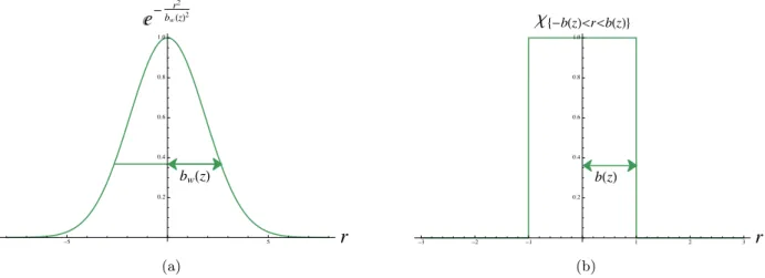
1.1 Water jet escaping (left) and trapping (right) in a sharp density transition. The experiments are fired with volumetric flow rate 15 mL/s,⇢b = 1.055 g/c.c.,⇢t= 1.043 g/c.c., ⇢j(0) = 0.998 g/c.c., where the Reynolds number Re'4600. The distance between nozzle and transition layer is 4 cm (left), and 12 cm (right). . . 3 1.2 (a) Gaussian jet/plume configuration (b) Top-hat configuration, for each fixed height
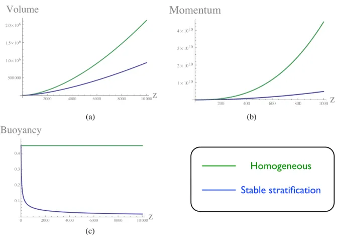
z. bw(z) and b(z) are reference radii of the jet or plume. . . 5 4.1 A comparison of mixing in ⇢0a(z) = (1.0037)(z+ 10) 3 and homogeneous ambient
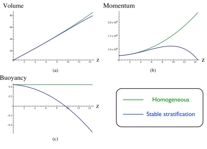
background densities. (a) Volume flux (b) Momentum flux increases for all distances (c) Buoyancy flux is always positive. . . 23 4.2 A comparison of mixing in linear and homogeneous ambient background densities.
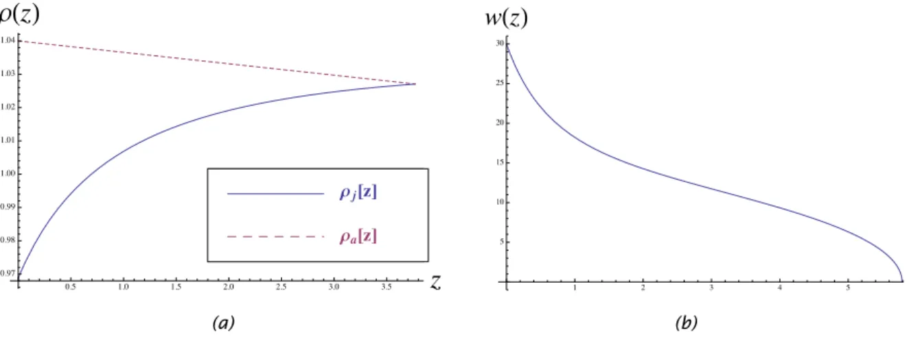
(a) Volume flux (b) Momentum flux, it can be seen that there is a maximum for momentum flux at the location of the neutral buoyant height, where the buoyancy flux vanishes. After this point it starts to decrease and eventually hits zero. (c) Buoyancy flux crosses zero and hence the system breaks eventually. . . 24 5.1 (a) Density of jet matches ambient atzne. Here the solid and dashed curves denotes
the jet density⇢j and ambient density⇢a, respectively. (b) Numerically calculated vertical velocity vanishes at zs. . . 32 5.2 Compare integral, series and numerical solutions with (a) Zero initial volume and
momentum fluxes. (b) All initial conditions being nonzero. . . 35 5.3 Neutral buoyant height formula (5.14) and the corresponding formula in [26] in terms
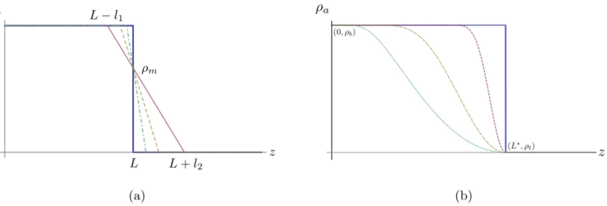
of ⇢b. . . 36 6.1 (a) Step function (thick) approximated by a series of constant-linear-constant profiles
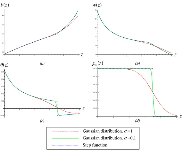
(solid, dashed, to dot-dashed) of increasing steepness of linear part. (b) A CSC approximation crossing the step function at density ⇢m (⇢t⇢m ⇢b). Steepness of linear part increases from solid to dashed to dot-dashed. . . 41 6.2 Numerically computed density anomaly,✓(z), with A Gaussian distribution function
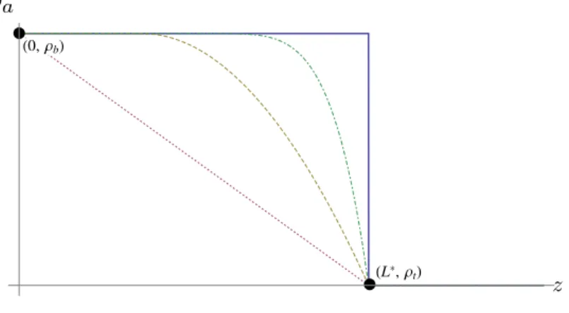
approximating delta function and imposing jump condition. . . 42 6.3 Two layer (thick) and linear (dotted), quadratic (dashed), quintic (dot-dashed) density
profiles decreasing from ⇢b to⇢t within distance L⇤. . . 45 6.4 The optimal mixing extends to step locationL less thanL⇤, that is, ⇢t>⇢j(L+)>
ˆ
⇢j(L+). . . 46 6.5 When the nozzle is placed at zjet 2 (0, L⇤) so that the z-coordinate is shifted as
6.6 Numerically computed jet density di↵erence⇢j ⇢j,l between two-layer and its linear stratification counterpart vs. distance from the nozzle, with jump location at L⇤;
parameters are: ⇢b = 1.057g/c.c.,⇢t= 1.045g/c.c. (solid),⇢t= 1.05g/c.c. (dashed). Curves terminate at neutral buoyancy position of each linear profile. Inset shows the
step and liner ambient density profiles for each parametric choice. . . 49
7.1 Experimental Setup . . . 51
7.2 Gear pump setup . . . 53
7.3 Syringe pump setup . . . 55
7.4 A nozzle holder that attaches to a slider so that the nozzle can be moved vertically. Labels A, B and C corresponds to items in Table 7.1. . . 56
7.5 Specification of conductivity probe adopted from manual. . . 58
8.1 Miscible buoyant-jet trapping/escaping critical-length vs. ⇢¯, with layer thickness also shown for each experiment. Curves: theoretical predictions. Symbols: experimental data. Non-dimensional length scale normalized by nozzle radius D(error-bars based on instrumentation).(a)L10data with L⇤m. (b)L90 data with L⇤. . . 60
8.2 Red profile: e↵ective two layer stratification. Blue profile: smoothed out profile with two-bucket mixing method for intermediate layers. Both profiles have the same density (1.0582g/cc) at the nozzle location 41.1 cm from the floor, and at 52 cm from the floor, with the same constant density of 1.0492g/cc at the top. The green squares and circles denote the locations ofL10 andL90 for the respective cases of the smooth and sharp transitions. The purple square is the location where the conductivity probe reads constant values for shallower depths for the sharp one. . . 62
8.3 (a) Water injected into the red profile shown in figure 8.2. (a) Water injected into the blue profile in figure 8.2. Clearly, the one injected into a sharply stratified environment trapped while injected in a less dense environment, the injection escaped. . . 62
8.4 (a) Green and Blue curves: Local ocean stratifications (by potential density) in DWH spill; Red and Black curves: concentration of hydrocarbons in water-column above well head (all from NOAA Technical Report, 2011); Purple (L⇤m) and Orange (L⇤): critical distances as a function of the formula’s top density, ⇢t, varying from the surface density '1.025g/cc to the maximum density at the well head'1.02774g/cc, using the entrainment coefficient, ↵ = 0.0833, as the release spill was extremely lightweight. Horizontal lines mark the intersections with ambient density. Orange prediction is a lower bound on trapping height, as it represents the optimal mixer. (b) Before L⇤(⇢t) intersects the ambient density profile (c) The special case where ⇢a(L⇤2) =⇢t2 (two curves intersects). . . 64
8.6 With identical background density profile and injection velocity, the jet with nozzle placed against the wall (a) clearly overshoots the one with nozzle in the middle of the tank (b). . . 66 8.7 (a) Numerically calculated Richardson number approaches the asymptotic valueq
16↵p2⇡/(5 ( 2+ 1)). (b) With⇢
b = 1.13, critical distanceL⇤ '6.5, and↵reaches 90% of↵p atz= 0.47. . . 68 8.8 (a) Numerically calculated Richardson number approaches the asymptotic valueq
16↵p2⇡/(5 ( 2+ 1)). (b) With⇢
b = 1.02, critical distanceL⇤ '0.8, and↵reaches 90% of↵p atz= 3.44. . . 69 8.9 After closing the three way valve, the dyed water leaks out from the nozzle owing to
buoyancy. . . 73 D.1 Schematic plot of the evolution ofznein terms of slope of the linear part. The colored
LIST OF TABLES
CHAPTER 1 INTRODUCTION
Mixing in stratified fluids is a topic of fundamental importance in nature. Of particular interest is the case in which mixing results in trapping phenomena, such as industrial smoke stack, volcanic eruptions, the accumulation of sinking marine snow (the solid carbon by-product of phytoplankton photosynthesis central to the carbon cycle) at density transitions [24], as well as trapping of pollutants in oil spills and other e✏uents in similar environments [4, 25, 36]. Here, we focus on the case of buoyant turbulent miscible jets (flow driven by momentum) and plumes (flow driven by buoyancy) in stable stratification (ambient density decreases with height) and the mixing e↵ects that results in subsurface trapping observable in such setups. A side remark on the di↵erence between jets and plumes in stably stratified environments is that even if initially the injection is a jet so that the buoyancy force (as a result of density di↵erences between injected and ambient fluids) is relatively small, eventually it will transition to a buoyancy dominated regime if a long enough free distance is given [12].
The Gulf of Mexico oil spill, for example, had crude oil injecting in the ocean at a very high flow rate, where the oil density is less than the whole ocean water. However, the ocean, owing to gradual lack of sunlight, is a density and temperature stably stratified environment so that even when oil is less dense than salt water, it entrains heavier fluid with itself when rising and when the e↵ective density of the oil-salt-water emulsion matches the density of its surrounding water, underwater oil plumes forms.
simplified from conservation of volume, momentum and buoyancy deficiency are: 8
> > > > < > > > > :
(b2w)0 = 2↵bw,
(b2w2)0 = 2g 2b2✓, (b2w✓)0 =⇢0
a(b2w)/(⇤⇢b),
(1.1)
where ↵, , ⇤ are constants to be discussed in chapter 2, ⇢a(z) is the ambient density profile. This system is valid for both jets and plumes, with a di↵erent selection of entrainment coefficient
↵ = ↵p (plume entrainment coefficient) or ↵ = ↵j (jet entrainment coefficient). Details of the setup, derivation and physical interpretations are in Chapter 2. There is a wealth of literature on buoyant turbulent jets, for example the classic text by Fischer et al., and more recent review articles by Woods, and Hunt & van den Bremer [12, 17, 39]. The oil spill incident fits in the framework of the MTT model, especially when bp sprayed corexit (an oil dispersant) to the wellhead. Corexit was supposed to allow the oil to be more rapidly degraded by bacteria, but meanwhile it made the oil miscible with water. The miscible oil-corexit-water emulsion is less dense than the ocean column, however the ability of carrying heavy water surrounding itself made it possible to increase the e↵ective density as a conglomerate, hence can be interpreted as injecting lighter fluid into a stratified environment, and how the entrainment and mixing changes the emulsion’s density, buoyancy, vertical velocity and volume are particularly interesting topics to focus on, and the MTT model is a suitable system to study for this setup.
Despite the extensive literature on this subject, many open questions remain, particularly regarding the mathematical foundation of predictions based on MTT models. We carry out a mathematically rigorous analysis of a broad class of MTT models, and experimentally verify their predictions.
1.1 Experimental results.
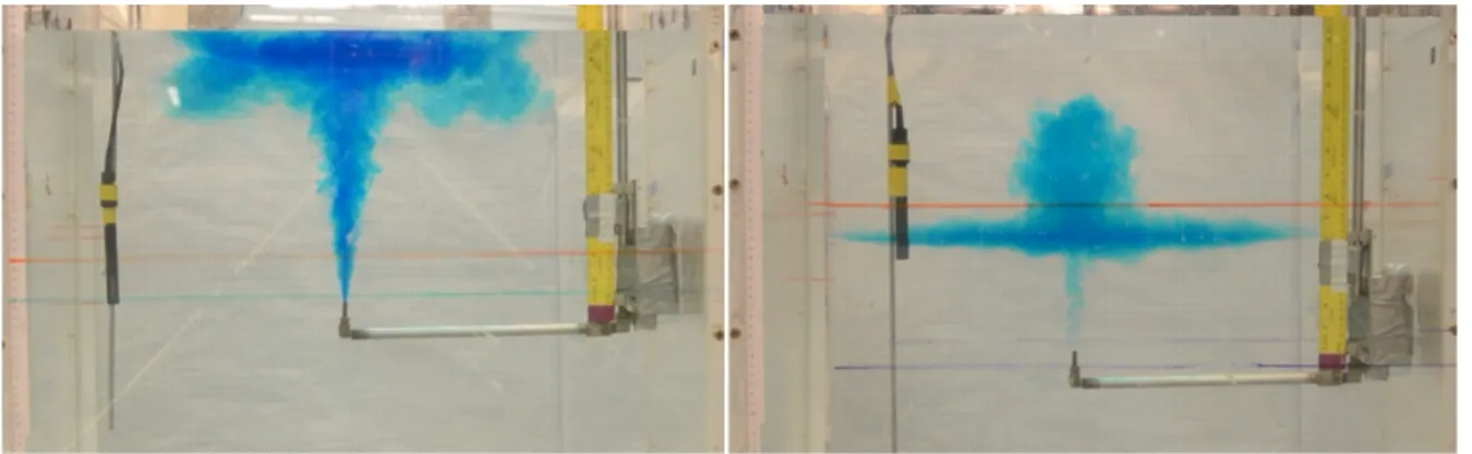
basic observation in these line-source studies was that strong penetration occurs when either the momentum is large or the stratification is weak. Here we focus on characterizing and measuring a critical phenomenon that can arise in such ambient fluid setups with three dimensional discharges: by varying the distance of the jet nozzle from a density transition, an experimental critical length is determined for which jets of any greater distances will be completely trapped, while jets with nozzles nearer the transition will escape. Figure 1.1 depicts typical trapping/escape outcomes in our experiments. Our experimental studies explore and document this criticality by demonstrating a sharp change in the trapping/escaping phenomena as the distance between the jet and density transition is varied by less than two percent.
Figure 1.1: Water jet escaping (left) and trapping (right) in a sharp density transition. The experiments are fired with volumetric flow rate 15 mL/s, ⇢b = 1.055 g/c.c., ⇢t = 1.043 g/c.c.,
⇢j(0) = 0.998 g/c.c., where the Reynolds number Re' 4600. The distance between nozzle and transition layer is 4 cm (left), and 12 cm (right).
1.2 Theoretical results.
After the MTT system was first introduced in 1956, many studies has been conducted based upon those equations, especially in density non-stratified environments. Power law solutions were derived with initial condition imposed at an imaginary virtual source lower than the actual nozzle location [28], predictions on apex heights and neutral buoyant heights with density profile being linear were also derived from dimensional analysis [35, 39]. Here a linear profile is
where ⇢2 the initial density,lis a prescribed location with density ⇢1, and ⇢2 >⇢1.
Our study here first focuses on a rigorous study on whether a MTT system with prescribed ambient density profile has a global solution or not, and it turns out that a breakdown of the solution corresponds to a trapping plume, while existing a global solution corresponds to an escaping plume. Once the breakdown/global existence criterion is established, we aim at calculating the neutral buoyant and apex height, especially in linear and step function ambient density stratifications. The step-like stratification can be written as
⇢a(z) = 8 > < > :
⇢b, z2[0, L),
⇢t, z 2[L,1).
(1.2)
The resulting formula for trapping and neutral buoyant heights in a linear stratification verifies the scaling law in [35, 39].
Furthermore, an exact formula for step-function stratifications employing non-linear jump conditions follows from this analysis. This formula favorably compares quantitatively with the data from an extensive experimental campaign to isolate the functional dependence of the critical distance with respect to the physical parameters. We remark that prior formulae, derived in [1], presented a critical height formula in homogenous background fluids; however, this result does not account for the important mixing which occurs when passing through the sharp background-density layer. The new formulae derived here take into account this critical additional strong mixing, resulting in an accurate prediction of the experimental critical lengths we observe.
Finally, our study provides a mathematically rigorous proof that under appropriate circumstances, step-like stratifications of the ambient fluid are the optimal mixers of the miscible jet fluid with the environment. That is, for fluid injected in step-like profiles, the density increment after entering the top layer is maximized compared to any other profile with the same density di↵erence within the same distance. The optimal mixing result is obtained through the direct comparison between the general system and the new exact solution (which now accounts for mixing in the layer) by using Gronwall-like estimates.
bwHzL
-5 5
r
0.2 0.4 0.6 0.8 1.0
„
-bwHr2zL2(a)
bHzL
-3 -2 -1 1 2 3 r
0.2 0.4 0.6 0.8 1.0 c8-bHzL<r<bHzL<
(b)
Figure 1.2: (a) Gaussian jet/plume configuration (b) Top-hat configuration, for each fixed heightz. bw(z) and b(z) are reference radii of the jet or plume.
a closer inspection shows that this is not always the case, depending on the self-similarity profile studied. The two commonly used configurations are Gaussian and Top-hat models [28], where the former assumes that vertical velocity and the density anomaly profiles are normal distribution curves centered about the axis of symmetry, and the later one assumes constant vertical velocity and density anomaly at each height from the centerline to the boundary of the injected fluid (see figure 1.2). Our analysis proves that the initial mixing by the Gaussian-profile closure model with a homogeneous background fluid is the weakest mixer amongst all stable stratifications. However, the extra mixing at the density step under this (Gaussian) closure restores the optimality of the two-layer stratification. The competition of weaker mixing in the bulk with enhanced mixing at the transition layer seems rather subtle and requires careful mathematical analysis. Alternatively, for the Top-hat closure, the higher contrast of jet density within a homogeneous lower fluid environment indeed results in the strongest mixing for distances shorter than the critical distance, and this comparison principle may break owing to the break down of the system for farther traveling distances.
1.3 Outline
An outline of this thesis is now given: A derivation of MTT model following the idea and assumptions made in [28] is given in §2.1, and a suitable rescaling of initial conditions of the MTT model is discussed, in order to have a fair comparison with the experimental outcomes.
which will be a convenient reference solution for further discussion on more general stably stratified environment. Owing to conservation of buoyancy flux, energy functionals governing the system can be found. We list two relevant energy functional that leads to equivalent exact solutions, and from those solutions a critical distance is derived.
We then study the general MTT model to establish mathematical criteria for solution existence and their finite-distance breakdown in §4.1. In§4.2, we derive sharper bounds for general ambient density profiles using Gronwall-like estimates, and study asymptotic behaviors in homogeneous background. We then apply these results to a family of stratification profiles of relevance for theo-retical and experimental investigations in§4.3. The estimates here and in§4.2 provide the rigorous framework for numerical observations in Caulfield & Woods (1998) reporting trapping/escaping criteria for a family of power-law density-height dependence. A final remark is given in the last part of this chapter, which shows that the eventual fate of an escaping plume must be straight-sided, with a slope 6↵/5, which was assumed in [22] to start an argument of the critical power for escaping plume to exist in a algebraic ambient density decay rate.
In Chapter 5, we focus on ambient density profiles with linear decay rates. The autonomous system with proper selection of variables has energy estimates well-established. An exact solution can hence be derived through this energy functional. A equivalent series solution was found in [32] and an integral solution was derived independently by [26]. The exact inverse integral solution is given in §5.1, and comparisons with solutions found in [26, 32] will be presented in§5.2 and§5.3.
An exact formula for the case of step density-height dependence is presented next, §6.1.1, under physically motivated jump conditions, which for their rigorous justification requires a study, carried out in§6.1.2, of linear stratifications (or more generally, by approximating the step function by a general family of smooth functions). The optimal mixer results for a broad class of stable stratifications, including their non-intuitive behavior dependence upon turbulent-closure choices, are presented in §6.2.
CHAPTER 2
CLASSICAL MORTON, TAYLOR, TURNER MODELS
2.1 Derivation of MTT models with general ambient density profile
Since turbulent mixing is a very complicated phenomenon which requires a wide range of length scales to be studied carefully. So, instead of attacking the full Navier-Stokes equations, reasonable simplifications is required to write down approximating equations governing turbulent mixing. To do that, researchers make assumptions on the nature of the rising jets or plumes so that the system can be simplified, for example, the entrainment hypothesis in section§2.1.1, and then justify the assumptions by experimental studies. Finally, one deduce results from the simplified formulation, and experimentally verify the results to build theories. In this section, we follow the idea of the original paper of MTT model [28] by introducing the relevant variables to be used, along with empirical observations that enables us to reduce the full system, and derive the MTT system in the following subsections.
The relevant time-averaged physical quantities in the MTT jet/plume system are the radius, vertical velocity and density anomaly of the jet/plume at each heightz, denoted by b(z, r), ¯w(z, r) and ✓(z, r) = (⇢a ⇢¯)/⇢b, respectively. Here ¯⇢ is the average density of the jet/plume and⇢a(z) is the ambient background density.
Experimental study of jets and plumes with Particle image velocimetry (PIV) and liquid laser fluorescence (LIF) shows that after a long-time averaging (or the steady state) of the vertical velocity and tracer concentration, those quantities are identical at each height in their radial direction [11, 12, 17]. This observation indicates that the time averaged variables are self-similar, that is,
¯
w(z, r) =wm(z)fw(r/bw(z))
✓(z, r) =✓m(z)f✓(r/bT(z)),
(2.1)
vertical velocity and density anomaly in the radial direction, respectively, andbw, bT are indicative radii of vertical velocity and tracer concentration distribution at each height.
There are two commonly used radially symmetric configurations [10, 12, 17, 28, 39]:
1. Gaussian configuration assumeswm(z) and✓m(z) are located at the centerline of the jet/plume for each height, and decays in the radial direction in a Gaussian distribution fashion:
¯
w(z, r) =wm(z) exp[ (r/bw(z))2],
✓(z, r) =✓m(z) exp[ (r/bT(z))2].
(2.2)
Here the width of the jet/plumebw(z) and bT(z) is selected such that the velocity and density anomaly reaches about 37% (1/e) of those along the centerline at each height, respectively.
2. Top-hat configuration, where the jet/plume is assume to have a constant vertical velocity at each height from the centerline to the boundary of the jet/plume, yielding a characteristic radiusb(z), and similar assumption was made for density anomaly, so that
¯
w(z, r) =wm(z) ({0rb(z)}),
✓(z, r) =✓m(z) ({0rb(z)}),
(2.3)
where is the characteristic function. See figure 1.2 for examples of the two configurations introduced above. Below we derive the conservation of volume, momentum and buoyancy fluxes along the centerline of the jet/plume based on the assumptions made according to experimental observations presented above.
2.1.1 Volume flux and entrainment hypothesis
flux equation. We start with defining the volume flux at each height of the injection as
q⌘
Z bw(z) 0
2⇡rwdr,¯ (2.4)
di↵erentiating in z
dq dz =
Z bw(z) 0
2⇡rdw¯ dzdr+
dbw(z)
dz 2⇡bw(z) ¯w(z, bw(z)), (2.5) and assuming the second term is negligible compared with the first term since w(z, r) ! 0 as r!bw(z), combining the incompressible equation in cylindrical coordinates derived in Appendix A
dq dz =
Z bw(z) 0
2⇡d(ru¯r)
dr dr= 2⇡ru¯r|r=bw(z), (2.6)
where ¯ur denotes the time-averaged radial velocity. Here an extra variable ¯ur was introduced. In order to close the system, the entrainment assumption proposed by Mortan, Turner and Taylor [28] enters the equation, which states that the radial inflow velocity at the boundary of the jet/plume is proportional to the vertical velocity along the centerline,
ru¯r|r!bw(z) =↵wm(z), (2.7)
here ↵is the entrainment coefficient, the proportionality constant described above.
The variableq can be written in terms of bw and wm by adopting the Gaussian configuration
q= Z 1
0
2⇡rw¯(z, r)dr= Z 1
0
2⇡rwm(z) exp[ (r/bw(z))2]dr=⇡(b2wwm)(z), (2.8)
On the other hand, when adopting the Top-hat configuration, the volume flux is
q= Z b(z)
0
2⇡rw¯(z)dr=⇡(b2wm)(z). (2.9)
In conclusion, the volume flux equation is:
dq dz =⇡
d dz(b
2
wwm) = 2⇡↵wm(z), (2.10)
or
dq dz =⇡
d dz(b
2w
m) = 2⇡↵wm(z), (2.11)
when adopting Gaussian and Top-hat configurations, respectively.
Since part of this study is aiming at the formation of underwater plumes, which requires the jet or plume to reach a state of negatively buoyant, which can be achieved by sufficient turbulent mixing of the injected fluid and the denser ambient fluid so that the densities of the two fluids match. But even when the injected fluid mixes to be neutrally buoyant, the momentum injected into the system forces the plume to overshoot the neutral buoyant height. Hence, in order to more precisely describe the jets or plumes behavior, the variation of vertical momentum and buoyancy must be studied, and governing equations will be derived in the next two subsections.
2.1.2 Momentum flux
Next, Consider the vertical momentum flux defined as
m= Z 1
0
2⇡rw¯2dr. (2.12)
Again, adopting Gaussian and Top-hat configurations, momentum fluxes can be written as
m= ⇡ 2b
2
wwm2, and m=⇡b2ww2m, (2.13)
✓ ur
@w
@r +w
@w @z ◆ = 1 ⇢0 ✓ @
@r(⌧rz) + 1
r(⌧rz) +
@
@z(⌧zz) (⇢ ⇢a)g
@(p p1)
@z ◆
,
where w is the vertical velocity, p p1 is the dynamic pressure distribution, p1 is the pressure remote from any disturbance, ⌧rz, ⌧zz are viscous stresses, ⇢, ⇢0 and ⇢a are jet/plume density, ambient density at the origin and ambient density profile that changes with height, respectively. Writeur= ¯u+u0 andw= ¯w+w0, whereu0 andw0 are fluctuations from the mean in time. Multiply the equation above by r and integrate from 0 to b(z) in r, the right hand side of the equation becomes
Z b(z)
0 rur
@w
@r +rw
@w
@zdr=r(¯u+u
0)( ¯w+w0)|
r=b(z)
Z b(z)
0
w@(rur)
@r wr
@w
@zdr (2.14)
with incompressibility, the first term in the last integration can be replaced by wr(@w/@z), and hence the right hand side of (2.14) equals
r(¯uw¯+u0w0)|r=b(z)+r(¯uw0+u0w¯)|r=b(z)+ Z b(z)
0 r @
@z( ¯w+w
0)2dr, (2.15)
expanding and the last term in the integration and integrate by parts Z b(z)
0 r @
@z( ¯w
2+w02)dr+ 2Z b(z) 0
rw¯@w0
@z +w
0@w¯ @zdr
= Z b(z)
0 r @
@z( ¯w
2+w02)dr+ 2Z b(z) 0
¯ w@(ru0)
@r +w
0@w¯ @zdr
= Z b(z)
0 r @
@z( ¯w
2+w02)dr 2(ru0w¯)|
r=b(z)+ 2 Z b(z)
0
ru0@w¯
@r +w
0@w¯ @zdr.
(2.16)
Substituting the last equation in (2.16) into (2.15) and average again in time so that every term with isolated u0 and w0 vanishes, so that (2.14) is simplified to
r(¯uw¯+u0w0)|r=b(z)+ Z b(z)
0 r @
@z( ¯w
Now the corresponding right hand side of (A.13) is Z b(z) 0 r ⇢0 ✓ @
@r(⌧rz) + 1
r(⌧rz) +
@
@z(⌧zz) (⇢ ⇢a)g
@(p p1)
@z ◆ dr = Z b(z) 0 1 ⇢0
@(r⌧rz)
@r +
r
⇢0 ✓
@
@z(⌧zz) (⇢ ⇢a)g
@(p p1)
@z ◆
dr,
(2.18)
combining (2.17) and (2.18) and multiply by 2⇡,
d dz Z b(z) 0 ¯
w2+ ¯w02+@(¯p p1) @z
¯
⌧zz
⇢0
2⇡rdr=
2⇡r(¯uw¯+u0w0 ⌧¯rz ⇢0 )
r=b(z)
+db(z) dz 2⇡b(z)
( ¯w2+ ¯w02+p¯ p1
⇢0 ¯ ⌧zz ⇢0 ) r=b(z) Z b(z) 0
2⇡rg ✓
¯
⇢ ⇢a
⇢0 ◆
dr,
(2.19)
where the over bars mean long time averaging the quantity. The first term on the right hand side is the momentum introduced by entrainment, and the second term is the axial momentum through the sloping sides of the jet/plume, and the last, integral term is the accelerating force per unit mass due to density di↵erence of the jet/plume and the ambient. A reasonably intelligent approximation was made by the following assumptions [12]:
1. The first two terms on the right of (2.19) are momentum carried into the jet/plume through entrainment, and axial momentum through the sloping sides of the boundaries. Generally, those two terms are assumed to be subdominant to the integral term, the total buoyancy flux across the horizontal area of the jet/plume.
2. Momentum flux from averaged vertical velocity is dominating the momentum fluxes generated from velocity fluctuations, pressure and viscous forces:
Z b(z)
0
2⇡rw¯2dr
Z b(z)
0
2⇡r ✓
¯
w02+p¯ p1 ⇢0 ¯ ⌧zz ⇢0 ◆ dr, (2.20)
so that the equation for vertical momentum flux with Gaussian configuration (2.2) is
d dz
Z 1
0
2⇡rw¯2dr= d dz(
⇡
2b 2
wwm2)⇡ Z 1
0
2⇡rg✓m(z) exp[ ( r bT(z)
while with Top-hat configuration (2.3), it becomes
d dz
Z 1
0
2⇡rw¯2dr= d dz(⇡b
2
ww2m)⇡ Z b(z)
0
2⇡rg✓m(z)dr=⇡gb2✓m. (2.22)
Here we replace the approximation sign in (2.20) and (2.21) by equal sign to write the momentum equations, which is a reasonable approximation to the averaged behavior of the turbulent mixing that the experimental data agrees with theoretical studies conducted in this research presented later.
2.1.3 Buoyancy flux (tracer concentration)
The rising velocity is decided by a combination of momentum and buoyancy e↵ects, so, to close the system, an equation describing ✓ must be included. Experimentally, density variations may not be measurable directly, in turn, convenient reference tracer concentration is used to back out the density information, hence an equation of tracer concentration is first derived which leads to density and buoyancy equation later. The time-averaged conservation of tracer concentration ¯C(r, z) is
r·( ¯Cu) = 0, (2.23)
which in cylindrical coordinates reads
1 r
@
@r( ¯Cu¯r) +
@
@zw¯= 0, (2.24)
so that the tracer concentration flux is
d dz
Z b(z)
0
2⇡rw¯Cdr¯ = 2⇡ru¯C¯ r=b(z)+db(z)
dz [ ¯wC¯]r=b(z). (2.25)
LetCa(z) be the ambient concentration of tracer, which is stratified in the vertical direction, and uniform on any horizontal plane. Combining this with the volume flux equation,
d dz
Z b(z)
0
2⇡rwC¯ adr= 2⇡ruC¯ a|r=b(z)+db(z)
dz [ ¯wCa]|r=b(z)+ dCa
dz Z b(z)
0
Finally, the concentration of tracer di↵erence flux equation can be given by the di↵erence of (2.25) and (2.26): d dz Z b(z) 0
2⇡rw¯( ¯C Ca)dr= dCa
dz Z b(z)
0
2⇡rwdr.¯ (2.27)
The relation of density anomaly and the tracer concentration anomaly is (¯⇢ ⇢0)/⇢0= ( ¯C C0)/C0, where is a constant, ¯⇢is the time averaged jet/plume density, and hence the equation for buoyancy flux is
d dz
Z b(z)
0
2⇡rw¯✓dr= d⇢a dz
Z b(z)
0
2⇡rwdr.¯ (2.28)
by selecting the reference density ⇢0 to be the maximum density of the whole system, ⇢b. For Gaussian configuration,
Z b(z)
0
2⇡rw¯✓dr= Z 1
0
2⇡rwm✓mexp ✓
r2( 1 b2 w
+ 1 b2T)
◆ dr=
✓
⇡ b
2 wb2T b2
w+b2T wm✓m
◆ , (2.29) so that d dz ✓ ⇡ b 2 wb2T b2
w+b2T wm✓m
◆
=⇡d⇢a
dz (b 2
wwm), (2.30)
and for Top-hat configuration, the governing equation is
d dz
⇣⇡ 2b
2w m✓m
⌘
=⇡d⇢a
dz (b
2wm). (2.31)
Equation (2.30) can be further simplified as
d dz ⇡⇤b
2
wwm✓m =⇡ d⇢a
dz (b 2
wwm), (2.32)
by adopting the empirical relationbT = bw [12, 28, 30], and let ⇤⌘ 2/(1 + 2).
2.1.4 Initial conditions
rescaled to conserve the initial fluxes. Denote by ¯b0, ¯w0 and✓0 the initial conditions in the Gaussian model, equating the initial volume, momentum and buoyancy fluxes with Gaussian configuration and their physical counterpart:
⇡¯b20w¯0 =⇡r02w0, 1 2⇡¯b
2
0w¯20 =⇡r02w20, 1 ⇤¯b
2
0w¯0✓0=r20w0 ⇢¯, (2.33)
where ⇢¯= (⇢b ⇢j(0))/⇢b, one finds that the initial conditions need to be rescaled by✓0= ⇢¯/⇤, ¯
w0= 2w0, ¯b0=r0/ p
2. Hereafter, initial conditions for the new variables will be defined by
Q0 = ¯b20w¯0, M0 = ¯b40w¯04, B0= ¯b20w¯0✓0, (2.34)
CHAPTER 3
HOMOGENEOUS AMBIENT DENSITY PROFILES
We begin by considering the reduced MTT model with Gaussian configuration derived above,
(b2w)0 = 2↵bw, (b2w2)0= 2g 2b2✓, (b2w✓)0 =⇢0a(b2w)/(⇤⇢b), (3.1)
where primes hereafter denote di↵erentiationd/dz. For notation simplicity, from now on we drop the upper bars and subscripts of the variables in §2.1 so that b(z) is the jet width, w(z) is the vertical jet velocity,✓(z) = (⇢a(z) ⇢j(z))/⇢b is the density anomaly. We also cancel the common constant⇡ on both sides of each equation. Here the constants are the gravitational acceleration g, the entrainment coefficient↵ and mixing coefficient [12, 28, 30]. With constant background density ⇢0a= 0, integrating the buoyancy flux equation yields b2w✓=B
0 so that it remains positive for all heights, which further guarantees global existence of solution to the MTT model (rigorous proved later in chapter 4). The corresponding MTT equation is
(b2w)0= 2↵bw, (b2w2)0 = 2g 2b2✓, b2w✓=B0, (3.2)
or by defining Qh=b2w,Mh=b4w4,B =b2w✓, the volume-momentum-buoyancy system is:
Q0h = 2↵M14
h, Mh0 = 4g 2B0Qh, B =B0. (3.3)
In the original paper [28], a set of power-law solution was given by assuming the b= Kbz↵b, w =Kwz↵w and ✓ =K✓z↵✓ and balance the power of the equations. It turned out that ↵b = 1,
↵w = 1/3, ↵✓ = 5/3, so that when z = 0 the solutions w and ✓ blows up that contradicts
location, one can find a corresponding virtual source (possibly very deep) location so that the system is well-posed. There are several di↵erent ways to determine the location of the virtual source to match the initial conditions at the nozzle height asymptotically, and a good summary can be found in [15]. The value of the power law solution is more about the far-field behavior of the plume: regardless of the location of the virtual origin, this solution set is the far-field asymptotic solution for homogeneous environments given as b ⇠ 6↵z/5, w ⇠ (25g 2B0/24↵2)1/3z 1/3, and
✓⇠ 625B2
0/1944g 2↵4 1 /3
z 5/3.
The power-law solution involves a selection of virtual origin, and the solution may not be accurate in short traveling distances. Hence, below we derive an exact integral solution to (3.2) for any positive initial conditions at the actual nozzle location (origin), and is the key to many general theorems in this research.
3.1 Exact integral solution
In [1], new variables = (w/✓)2 and = 1/✓ were introduced and the equations can be derived as the following:
d dz =
⇣ b2w2
b2w✓·✓/w
⌘0
=⇣b2Bw2
0
p ⌘0
=⇣2g 2b2✓p +b2w2 0 1/2/2⌘/B0 = 2g 2b2w+B0 0/2 /B0 = 2g 2/✓+ 0/2,
(3.4)
Hence 0 = 4g 2 . Similarly,
d dz =
⇣ b2w
b2w✓
⌘0
= 2↵Bbw
0 =
2↵bpw✓pw B0p✓ =
⇣ 2↵ p B0 ⌘ 1/4 (3.5)
so that the first two equations of (3.2) become
d
dz = 4g
2 , d dz = ✓ 2↵ p B0 ◆
1/4, (3.6)
Dividing the two equations and separating variables yields the conserved quantity
2 =⇣ 4↵ 5pB0g 2
⌘
Imposing initial conditions determinesA=✓02 4↵w¯2
0/(5g 2¯b0✓30), where ¯w0,✓0,¯b0 are the initial conditions in (2.34). Substituting (3.6) back into (3.7) and separate variables again yields
z= 1 4g 2
Z
0
ds p
as5/4+A, (3.8)
where a= (4↵/5g 2pB0).
On the other hand, a new conservation quantity governing system (3.3) can be establish by the following :
Qh =
Q20+ 4↵ 5g 2B
0 ✓ M 5 4 h M 5 4 0 ◆ 1 2 , (3.9) so that
z(Mh) = 1 4g 2B
0 Z Mh
M0
Q20+ 4↵ 5g 2B
0 ✓
s54 M 5 4 0 ◆ 1 2 ds, (3.10)
orz in terms of volume flux Qh:
z(Qh) = Z Qh
Q0 1 2↵ M 5 4 0 +
5g 2B0 4↵ s
2 Q2 0
1 5
ds. (3.11)
The two expressions of exact solutions above will be studied in depth as several solution existence range results are obtained by comparing with those formulas. The later conservation law can be generalized to the case of linear ambient background density profiles, and the expression (3.11) is particularly helpful for deriving the far field asymptotic relations. The far field asymptotic behavior is particularly important to determining whether systems breakdown or not. Before proceeding to general theories, a critical distance formula can be directly given as an application of the exact solution.
3.2 Matching critical distance L⇤m
choosing ⇤m =⇢b/(⇢b ⇢t), ⇤m= nh
(⇢b/(⇢b ⇢t))2 A i
/ao4/5. The formula is given as
L⇤m= 1 4g 2
Z ⇤m 0
ds p
as5/4+A, (3.12)
and equivalently, by selectingQ⇤m = (B0⇢b)/(⇢b ⇢t) and use (3.11),
L⇤m= Z Q⇤m
Q0
1 2↵
M
5 4
0 +
5g 2B0 4↵ s
2 Q2 0
1 5
ds. (3.13)
Now under an identical setup but replace the constant ⇢b density profile to a two-layer system
⇢a(z) = 8 > < > :
⇢b zL,
⇢t z > L,
and consider the two cases:
1. L L⇤m, ⇢j(L) >⇢t, hence passing through the layer, the jet has already been negatively buoyant and must trap, whereas
2. L L⇤m, the jet density after entering the homogeneous top layer is still less than ⇢t, and must rise indefinitely.
CHAPTER 4
GENERAL THEORY FOR MTT MODELS
4.1 Model and solution existence criterion
Now back to the general stably stratified MTT system:
q0 = 2↵m14, m0 = 4g 2q , 0 =⇢0
aq/(⇤⇢b), (4.1)
describing the volume, momentum, and buoyancy fluxes, respectively. First we establish a criterion for global solution to exist or the system breaks down in finite distances.
Existence/Break down theorem
Theorem 4.1.1(Existence/Break down). Letzsbe the location where momentum vanishes,m(zs) =
0 and zne be the neutral buoyant height, (zne) = 0. For a stably stratified environment (⇢0a0),
the solution to (4.1) exists in [0, zs), provided the initial values of q(0) = Q0, m(0) = M0 and
(0) = B0 are all positive. Furthermore, if zne < 1 and 0(zne) < 0, then zs < 1, that is, the
system breaks down in finite distances.
The proof of existence is divided into two regions – [0, zne] and [zne, zs) – wherezne is the neutral buoyant location ( (zne) = 0).
The existence of solutions can be established by the bounds
Q0 q 2Q0eKz, M0 mM0sinh(Kz), 0 B0 in [0, zne], Q0 q 2Q0eKz, 0< mm(zne), 1< 0 in [zne, zs),
(4.2)
[0, zne], so thatmis increasing,m M0 >0, by the momentum equation in (4.1). Forz zne, note thatznealso plays the role of locating where the maximum momentum occurs, since mis decreasing after zne; for as long asm does not decrease to zero, q keeps increasing, and keeps decreasing.
Proof of Theorem 4.1.1.
Case 1. z2[0, zne]
Upper bounds for q and m are sufficient to show existence in [0, zne], as 0 B0.
Non-dimensionalising theq andmequations in (4.1) byq¯= q/Q0,m¯ =m/M0, the di↵erential inequalities
follow 8
> > < > > :
¯
q0 = 2↵M
1 4 0
Q0 m¯ 1
4 2↵M
1 4 0
Q0 m¯
¯
m0 = 4g 2 Q0
M0 q¯
4g 2B0Q0
M0 q,¯
(4.3)
with the inequality in the first line holding since m >¯ 1 in [0, zne]. Comparing system (4.3) with
the linear systemQ0b =KMb, Mb0=KQb, yields (See [33] or simply solve the di↵erential inequality
with separation of variables.)
Q0q Q0
2 ⇥
eKz+e Kz⇤=Qb(z),
M0 m M0
2 ⇥
eKz e Kz⇤=Mb(z),
(4.4)
so that q and m have upper and lower bounds in any finite interval [0, zne].
Case 2. z > zne
Forz > zne,mdecreases, and the bounds forqin (4.4) hold untilm(zR) =M0for somezR2(zne, zs).
However, another di↵erential inequality holds: q¯0 2↵M14
0/Q0 for z zR, hence q Q(zR) +
KQ0(z zR). Stitching the two bounds together, and noting that by (4.4), Q(zR)Q0exp(KzR),
with Q0K(z zR) < Q0exp(K(z zR)), an upper bound for q is 2Q0exp(Kz) forz zR. Note
thatQb 2Q0exp(Kz), so that an overall bound for q can be found:
In summary, for z > zne, m decreases, and as long as m stays positive, 0 < m < m(zne),
Q0 q2Q0exp(Kz), and | | also does not blow up in finite heights z since q has a smooth lower
bound,
B0 =B0 Z z
0
|⇢0a|
⇤⇢b
qds B0 Z z
0
2|⇢0a|Q0 (⇤⇢b)
eKsds > 1,
so that solution existence can be extended to [zne, zs).
Sincem0 = 4g 2 q <0 atz
s, which forcesq0 = 2↵m1/4 to become complex. Note that if never touches zero, the solution is global sinceq andm are increasing and bounded by the first estimate in (4.2), while is decreasing with zero lower bound.
Furthermore, if zne < 1 and 0(zne) < 0, there exists z > zne such that (z ) < < 0 for some negative number , integrating the di↵erential inequalitym0= 4g 2q <4g 2Q0 from z to anyz > z yieldsmM(z ) + 4g 2Q0 (z z ), which implies that mmust be zero within a finite distance z⌘zs.
Figure 4.1 and 4.2 demonstrates escaping and trapping. In this numerical simulation, linear stratification is adopted as an example of a stable stratification.
4.2 Main bounds and asymptotic relations
Lemma 4.2.1. Let (Qh,Mh, B0) be a set of solutions to (3.3) and (q, m, ) be a set of solutions
to (4.1), with identical initial conditions Q0, M0 andB0, then the following relation holds:
q Qh, mMh, B0. (4.5)
Proof. Sharper bounds forq and in system (4.1) can be derived by using a Gronwall-like estimate:
since B0, integrating the inequality inq,
2↵m14dm
dq = 8↵
5 dm54
dm dm
dq 4g 2B
0q, (4.6)
yields the relation
m(q) ✓
5g 2B 0 4↵ (q
2 Q2
0) +m(Q0)
5 4
◆4 5
2000 4000 6000 8000 10 000z 500 000
1.0¥106 1.5¥106 2.0¥106
Volume
200 400 600 800 1000
z
1¥1010 2¥1010
3¥1010 4¥1010
Momentum
0 2000 4000 6000 8000 10 000
z
0.10.2 0.3 0.4
Buoyancy
Homogeneous
Stable stratification
(a) (b)
(c)
Figure 4.1: A comparison of mixing in ⇢0a(z) = (1.0037)(z+ 10) 3 and homogeneous ambient background densities. (a) Volume flux (b) Momentum flux increases for all distances (c) Buoyancy flux is always positive.
Solving for q in (4.1) using the inequality above yields the estimate
Z(q)⌘ 1 2↵
Z q
Q0
✓ 5g 2B
0 4↵ (s
2 Q2
0) +m(Q0)
5 4
◆ 1 5
dsz(q). (4.8)
2 4 6 8 10 12 14
z
2040 60 80
Volume
2 4 6 8 10 12 14
z
-0.4
-0.2 0.2 0.4
Buoyancy
Homogeneous
Stable stratification
2 4 6 8 10 12 14
z
1.0¥106
1.5¥106 2.0¥106
Momentum
(a) (b)
(c)
Figure 4.2: A comparison of mixing in linear and homogeneous ambient background densities. (a) Volume flux (b) Momentum flux, it can be seen that there is a maximum for momentum flux at the location of the neutral buoyant height, where the buoyancy flux vanishes. After this point it starts to decrease and eventually hits zero. (c) Buoyancy flux crosses zero and hence the system breaks eventually.
yields the relation
m=M0+ Z z
0
4g 2 qdsM0+ Z z
0
4g 2B0Qhds=Mh. (4.9)
To conclude, q(z)Qh(z) andm(z)Mh(z) provided the solution to equation (4.1) exists. Lemma 4.2.2. Let (Qh, Mh, B0) be a set of solutions to (3.3) with positive initial data (Q0,
M0, B0), Qh ⇠ C1B01/3z5/3, Mh ⇠ C2B04/3z8/3 as z ! 1, where C1 = 1944g 2↵4/625 1/3,
The asymptotic relation above can be found by using the inverse integral solutions of (3.2), viewed as functions ofQh and Mh, respectively,
z(Qh) =
(Qh Q0)
4 5 2↵ Z 1 0 ✓ M 5 4 0 +
5g 2B0
4↵ r(2Q0+ (Qh Q0)r)
◆ 1 5
dr, (4.10)
z(Mh) =
Mh M0 4g 2B
0 Z 1
0 ✓
Q20+ 4↵ 5g 2B
0
((M0+ (Mh M0)r)
5 4 M 5 4 0 ) ◆ 1 2
dr . (4.11)
The derivation of those asymptotic relations are in Appendix B. Note that following the previous argument, if a priori it is known that > 1>0, a lower bound forq can be obtained by
1 2↵
Z q
Q0
✓
5g 2 1 4↵ (s
2 Q2
0) +m(Q0)
5 4
◆ 1 5
ds z(q), (4.12)
and since m(Q0) andQ0 are positive, by changing variabless=Q0+ (q Q0)r, it follows that
z(q)< (q Q0)
4 5
(40g 2↵4
1)
1 5
Z 1
0
(r(2Q0+ (q Q0)r))
1
5 dr < q Q0
C1 11/3
!3 5
. (4.13)
Thus, a lower bound for q can be found
q(z)> C1 11/3z5/3. (4.14)
Figure 4.1 and 4.2 demonstrates that the volume, momentum and buoyancy fluxes in homogeneous ambient are upper bounds for those in stably stratified environments.
4.3 Analytical trapping-escaping criterion for more general profiles
For special types of density profiles, a prior estimates on the location ofzneis useful for determining whether a system breaks down or not. For example, Caulfield and Woods (1998) proposed the following theorem based on numerical evidence [7]:
Critical exponent for algebraic density decay rates
(C <0), a critical power p = 8/3 separates two distinct behaviors: if p > 8/3, the jet/plume
must trap while for p < 8/3 either trapping or escaping could happen.
Note that this constant is set by the overall density di↵erence if the power-law dependence on z is strictly imposed throughout the domain, and in the later case, whether trapping or escaping will be determined by the magnitude of |C|. We will prove this result analytically below, and, as a corollary, also show that the result extends to more general profiles:
Corollary 4.3.1. In system (4.1), for ambient density functions ⇢0a⇠Czp as z! 1, the critical exponent result in Theorem 4.3.1 also holds.
We remark that this critical behavior, which was originally observed numerically by [7], have been recently investigated by [22] using formal asymptotic tools which have provided a partial insight this phenomenon. This study, under the restrictive assumption that the plume is straight sided (purely conical) and by assuming infinite existence domain for the solution, successfully yields the critical exponent p= 8/3 obtained by [7]. Our results below use integral estimates to achieve mathematical rigor and avoid formal assumptions; the techniques we use further extend and prove the existence of this critical behavior for a much broader class of background density profiles.
To construct a rigorous mathematical proof we use the solution existence criterion established in §4.1: since ⇢0a ⇠Czp asz! 1, for z large enough, 0 must be strictly negative so that if z
ne is finite, must be less than some value <0. Hence, by Theorem 4.1.1, existence of finite zne implies breakdown of the system, which means trapping must occur. Conversely, if > 0, the solution of (4.1) is global and the injection rises indefinitely.
Proof of Theorem 4.3.1.
Case 1. Trap as p 8/3
Suppose >0 for all z; since is monotonically decreasing, then ! 1 0 as z! 1. and
⇢0a ⇠ Czp for p 8/3 as z ! 1 implies ⇢0az5/3 2/ L1(R+). With
1 0, either 1 > 0, or
1= 0.
Case 1.1. 1>0
B0 C1 ⇤⇢b
Z z
0 |
⇢0a| 11/3z5/3ds <0, (4.15)
Case 1.2. 1= 0
If 1= 0, the above lower estimate for q fails. However, in this case, the estimate below shows
that there must exist zne<1 such that (zne) = 0. To show this, it is sufficient to estimate q for
finite z: when 1= 0, for any fixed zc <1, (zc) = c >0. Confining z2[0, zc), and follow the
same steps above, we have q(z)> C1 c1/3z5/3=C1 (z)1/3z5/3. The equation in (4.1) thus yields
(z) 23 B 2 3
0 2 3
✓ C1 ⇤⇢b
Z z
0 |
⇢0a|s53ds
◆
(4.16)
and since R01|⇢0a|s53ds = 1, there must exist zne < 1 so that (2C1/3⇤⇢b)Rzne
0 |⇢0a|s
5
3ds = B0.
On the other hand, combining the assumption 1= 0 with (4.16) one concludes a contradictory
inequality: 0 = ( 1)2/3<( (zne))2/3 0. Hence zne must be finite, and trapping must occur.
Case 2. p > 8/3, ⇢0az5/3 2L1(R+) Case 2.1. Escape
If p > 8/3, since qQh (details in §4.2), with Qh the solution to the system of equations with
homogeneous ambient density (3.2), we have the following estimate on :
(z) =B0+ Z z
0
⇢0a
⇤⇢b
qds B0 Z z
0
|⇢0a|
⇤⇢b
Qhds. (4.17)
Since we know Qh ⇠C1B01/3z5/3 as z ! 1 (see §4.2), a sufficiently small |C|prevents = 0 at
finite distances and leads to escaping.
Case 2.2. Trap
On the other hand, for large values of |C|, through estimate (4.16), again forces trapping as (z)
vanishes for some finite value z.
4.3.2 Straight-sided plumes
escaping eventually will be straight-sided, that is, the radiusb(z)⇠C3z asz! 1, where C3 is a positive constant. Then, solve an equivalent system asymptotically and finally obtain the critical power for which the straight-sided assumption could exist. Here we show that the assumption of straight-sided plume made in [22] must hold if the plume escapes and that C3 = 6↵/5. By §4.3, we know that an escaping plume must have a non-negative limit in buoyancy flux. Again, we first assume that 1 >0, and notice that q ⇠ C1 11/3z5/3, m ⇠C2 14/3z8/3 as z ! 1 (derived
in Appendix B) so that b(z) = q/m1/4 ⇠ C
CHAPTER 5
EXACT SOLUTIONS FOR LINEAR AMBIENT DENSITY PROFILE
A linearly decreasing density profile can be poured for prescribed initial and terminal density within a preselected distance by the two-bucket method described in the experimental section in Chapter 7, it is a good reference profile when a non-homogeneous environment is of interest. An extension of linear profile is a connection of constant density profiles, for example, a constant-linear-constant profile, which expands the family of ambient density stratifications one is interested in studying.
Suppose that the background density is linear:
⇢a(z) =⇢b+ (⇢t ⇢b) z
L (5.1)
where ⇢a(z) is the background density, ⇢b,⇢t are the density of fluid at the bottom and top of the environment we care about, andLis the depth of the ambient fluid. The MTT model with (5.1) has been studied by Scaseet al. [32] as a steady plume of their time-dependent equations, and derived a series solution. Mehaddi et al. [26] also attacked this equation with Top-hat configuration by introducing the variables (z), the Richardson number [16, 27], and (z), the Buoyancy frequency parameter [3]. An exact inverse integral solution was derived through those variables, and hence the plume neutral buoyant and rise height can be calculated.
will be given in Chapter 6.
First we consider an idealized linear profile for z > 0. In terms of the original volume and buoyancy fluxes and the square of Momentum flux, the MTT model is a system governed by energy estimates, and yields a set of inverse integral solutions.
5.1 Exact solution, neutral buoyant and trapping height
We denote the MTT model with linear ambient density profile as
Q0l = 2↵M
1 4
l , Ml0 = 4g 2QlBl, Bl0 = N2Ql, (5.2)
where the constant buoyancy (Brunt-V¨ais¨al¨a) frequency isN2 = ⇢0a/(⇤⇢b) = ⇢⇤b⇢b⇢Lt. By the second and third equation of (5.2) we know that
dMl dBl
= N
2Q l 4g 2Q
lBl
= N
2
4g 2B l
, (5.3)
by separation of variables, a relation between momentum and buoyancy fluxes is established:
2g 2Bl2 = N2Ml+ [N2M0+ 2g 2B02], (5.4)
where the initial conditions are Ql(0) =Q0 =b02w0,Ml(0) =M0 =b40w40,Bl(0) =B0=b20w0✓0. Define CB⌘N2M0+ 2g 2B02 >0, by (5.4):
Ml=
CB 2g 2Bl2
N2 . (5.5)
Plug this relation in the first equation of (5.2), the other conservation law is obtained by:
dQl dBl
= 2↵M
1 4
l N2B
l
, (5.6)
again, by separation of variables:
N2 2 (Q
2
l Q20) = 2↵
p N
Z Bl B0
(CB 2g 2r2)
1
Further calculation yields: Z Bl
0
(CB 2g 2r2)
1
4dr = (CB)14
Z Bl 0
(1 2g 2
CB
r2)14dr (5.8)
= (CB)
1 4Bl
Z 1
0
(1 2g 2
CB
Bl2s2)
1
4ds (5.9)
by letting s= Br
l. Again, by change of variablesr=s 2: Z Bl
0
(CB 2g 2r2)
1
4dr = (CB)
1 4Bl
2
Z 1
0
(1 2g 2
CB
B2lr)14r 1
2dr (5.10)
= (CB)14Bl[2F1( 1
4, 1 2,
3 2,
2g 2 CB
Bl2)],
where 2F1( 14,12,32,2g
2
CB B 2
l) is a hypergeometric function. Define H(B) ⌘2F1( 14,12,32,2g
2
CB B 2 l), the conservation relation between Ql and Bl is:
Ql={ 4↵
N52
[(CB)14(Bl·H(Bl) B0·H(B0))] +Q2
0}
1
2. (5.11)
Combine with the third equation of (5.2), we have:
Bl0 = N2{ 4↵ N52
[(CB)
1
4(Bl·H(Bl) B0·H(B0))] +Q2
0}
1
2 (5.12)
this leads to a exact relation:
z= 1 N2
Z Bl B0
{ 4↵
N52
[(CB)
1
4(r·H(r) B0·H(B0))] +Q2
0}
1
2dr. (5.13)
From these exact relations, we are able to calculate the neutral buoyant and trapping height of fluid released from the bottom of the container:
z{ne,s} =
1 N2
Z B⇤
B0
{ 4↵
N52
[(CB)14(r·H(r) B0·H(B0))] +Q2
0}
1
2dr, (5.14)
where B⇤ = 0 or q CB
2g 2, respectively. Those are selected as above since B(zne) = 0, and if zs satisfies w(zs) = (
p
1 2 3 4 5
z
5 10 15 20 25 30w
H
z
L
(a) (b)
0.5 1.0 1.5 2.0 2.5 3.0 3.5
z
0.97 0.98 0.99 1.00 1.01 1.02 1.03 1.04
r
H
z
L
ra@zD
rj@zD
Figure 5.1: (a) Density of jet matches ambient at zne. Here the solid and dashed curves denotes the jet density ⇢j and ambient density⇢a, respectively. (b) Numerically calculated vertical velocity vanishes atzs.
Q0 Q2Q0eKzs, we know thatM(zs) = 0. The relation (5.4) further yields B2 = (CB/2g 2) as M = 0, and hence B⇤ = p(CB/2g 2). Note that B⇤ is selected with the negative square root since by (5.2), ifB 0,M is an increasing function, and henceM M0 >0. In other words, if M(zs) = 0,B(zs) must be negative. Figure 5.1 demonstrates the validity of those two formulas by numerically solving a system in the range [0, zne] and [0, zs], .
5.2 Comparison with series solution by Scase et al.
In [32], a similar energy estimation was proposed and from there, by inductively balancing the dominating order of two sides of the di↵erential equations, a series solution is derived under several di↵erent types of initial conditions. Here, starting from the exact solution (5.13), we show that the two solutions are equivalent.
Note that without expressing (5.13) with a hypergeometric function, it can be written as
z= 1 N2
Z Bl B0
✓
Q20 4↵ N52
Z s
B0
(CB 2g 2r2)
1
4dr
◆ 1 2
ds. (5.15)
In the case Q0 = M0 = 0, z(Bl) = 1 (4↵p⇢0)12N34
RB0
Bl
df r
RB0
f (B02 g2) 1 4dr
(B0 f)v+f,f = (B0 Bl)u+Bl gives:
z(Bl) =
1 (4↵p⇢0)
1 2N 3 4 Z 1 0
(B0 Bl)
3
8(1 u)58du
qR1
0[(B0+Bl) + (B0 Bl)(u+ (1 u)v)]
1
4(1 v)14dv
.
To study the asymptotic behavior as Bl !B0, let ✏=B0 Bl >0, and observe
z(Bl,✏) =
1 (4↵p⇢0)
1 2N 3 4 Z 1 0
✏38(1 u) 5 8
Z 1
0
[(B0+Bl) +✏(u+ (1 u)v)]
1
4(1 v)14dv] 1
2 du
as✏!0+. Defining
I(Bl,✏) = Z 1
0
✏38(1 u) 5
8 du
qR1
0[(B0+Bl) +✏(u+ (1 u)v)]
1
4(1 v)
1
4dv
, (5.16)
the asymptotic relation I(Bl,✏)⇠(✏3/8p5)/(29/8(B0)1/8)(8/3 + 5✏/(198B0)), as ✏!0. (Appendix B.1) yields
z(Bl,✏)⇠
✏3/8p5
(4↵p⇢0)12N3429/8(B0)1/8
(8 3 +
5✏
198B0
). (5.17)
5.2.1 Method of dominant balance
In order to invert our inverse integral solution and write out a series solution to compare with the one derived in [32], method of dominant balance is applied with the expression (5.17) as z!0. Let
✏=a1z
8
3 +a2z163 =a1z83(1 + a2
a1z 8
3), and observe the leading order in terms ofz:
p
2(4↵2⇢0N3)
1
4z = (a1z
8
3 +a2z
16
3 )
3
8p5
2
1 (2B0)
1 8
[8 3+ (
5 2·9·11B0
)(a1z
8
3 +a2z163 )]
⇠ (a
3 8
1z+ (8a2/3a1)a
3 8
1z
11
3 )p5
2
1 (2B0)18
[8 3 + (
5 2·9·11B0
)(a1z
8
3 +a2z
balancing orders z and z113 :
O(z) :p2(4↵2⇢0N3)
1
4 =a
3 8 1 p 5 2 1 (2B0)18
8 3;
O(z113 ) : 8a2
3a1 a38
1 = ( 5 2·9·11B0
)a1+38
1 ,
givesa1 = 2
11
3 ·3
8 3·5
4
3 ·B0[(4↵2N3
B0 ) 1 4]
8
3,a2= 2
25
3 ·3
10
3 ·5
5
3 · 1
11·B0[(4↵
2N3
B0 ) 1 4]
16
3. Those constants
agrees with the expansion obtained in [32].
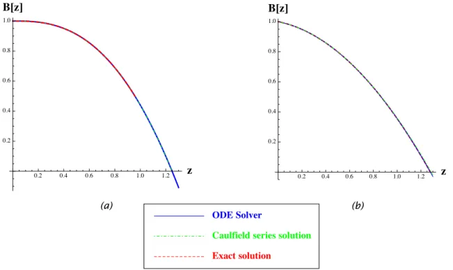
Note that the analysis above sets Q0 = M0 = 0 and B0 6= 0, which is a non-physical initial condition since this implies✓0 =1. It can only be rationalized without tracing back to the original variablesb, w and ✓, or by approximating a pure plume release, that is, buoyancy is the initial dominated force so that momentum and volume fluxes are neglected. Also notice that in this case, Ml1/4 is notLipschitz continuousso that uniqueness of solution cannot be guaranteed. A trivial solution (Ql, Ml, Bl) = (0,0, B0) can be found [32], and in order to compare the nontrivial solution (5.13) and series solution with numerical solution, a perturbation of initial data on Q0 = 10 8 is applied in figure 5.2. Furthermore, ifM0 is positive, the analysis is simpler since every term on the right hand side of equation (5.2) is C1 at z= 0, and hence the series solution is actually the
Taylor expansion at z= 0 and the Taylor coefficients can be found by continuously di↵erentiating Ql,Ml,Bl at the initial point. (The non-physical initial conditions in Figure 5.2 (a) and (b) are: (Q0, M0, B0,) = (10 8,0,1,1) and (1,6,1,0.4).
5.3 Comparison with Integral solution by Mehaddi et al.
Independently, Mehaddiet al. [26] found an inverse-integral solution to MTT model with linear ambient background density profile, by studying a di↵erent set of variables, the Richardson number, the buoyancy frequency parameter and radius, denoted by = (5gb✓/8↵w2), = (N2w2/g✓2) and
b. Equations are 8
> > > > > > < > > > > > > :
0= 4↵
b ⇥
1 1 +25 ⇤,
0 = 16↵
5b ( + 1), b0 = 45↵ 52 .
Exact solution
Caulfield series solution ODE Solver
(a) (b)
0.2 0.4 0.6 0.8 1.0 1.2 z 0.2
0.4 0.6 0.8 1.0
B@zD
0.2 0.4 0.6 0.8 1.0 1.2 z 0.2
0.4 0.6 0.8 1.0
B@zD
Figure 5.2: Compare integral, series and numerical solutions with (a) Zero initial volume and momentum fluxes. (b) All initial conditions being nonzero.
Note that in linear ambient profiles, the injection must eventually trap (by §4.3), so that✓= 0 somewhere, which leads to = 0 and hence attains its maxima at the same point. Writing the inverse integral solution in terms of z( ) will be impossible since functions are not invertible at an extrema. The cure is to write out the whole solution into two ranges divided by this critical point. In our case, we by passed this complication by studying instead the buoyancy flux, which is a monotone decreasing function and hence invertible. Figure 5.3 demonstrates that when calculating the neutral buoyant height using the two formulas (5.14) and the one derived from (5.3), for ⇢b between 1.01g/c.c and 1.11g/c.c, and ⇢t=⇢b 0.012, the two curves are identical.
1.02 1.04 1.06 1.08 1.10 rb 2
3 4 5 6
Neutral Height@rbD
Mehaddai et al.zneformula zneformulaH5.14L
Figure 5.3: Neutral buoyant height formula (5.14) and the corresponding formula in [26] in terms of
⇢b.
CHAPTER 6
TWO LAYER AMBIENT DENSITY PROFILES
6.1 Jump condition and critical formula
Di↵erent from the background density profiles discussed above, a profile with a sharp change in density is studied in those type of setups in this chapter. Layers of drastic change in density (halocline) or temperature (thermalcline) can be found in the ocean and are important in several climate aspects, for example, in high latitude regions they played an important role on formation of sea ice, and prevents the escape of carbon dioxide to the atmosphere [2]. Strong salinity gradient in deep water, for instance, in Gulf of Mexico has also been observed as brine pool [20], which maintains a stable stratification.
Mixing in stratified fluids is the main focus of this study, especially in naturally occurring, sharply stratified environments described above. In this case, the rising jet bifurcates at a critical distance L⇤ into two outcomes - for nozzle located closer to the transition layer than L⇤, the jet escapes while farther thanL⇤ it traps. Note that with this sharp transition in ambient density leads to a nonlinear jump in the equation at the layer location, hence a physical condition is required to define the solution.
The importance of this type of stratification is not restricted to the observable critical change of trapping/escaping, it is also the density profile that increases the density of a rising fluid the most. This result can be applied to estimate behaviors of various di↵erent density stratified environments.
6.1.1 Exact formula with two-layer ambient profile
We now focus on a generalized MTT system for the behavior of a turbulent jet/plume in a sharply stratified ambient fluid (represented by a step function,⇢=⇢b forz < Land ⇢=⇢t whenz > L),
![Figure 5.3: Neutral buoyant height formula (5.14) and the corresponding formula in [26] in terms of](https://thumb-us.123doks.com/thumbv2/123dok_us/8230361.2181807/48.918.129.800.123.391/figure-neutral-buoyant-height-formula-corresponding-formula-terms.webp)