Equivalent
Models in the
Context of
Latent
Curve
Analysis
Diane Losardo
A thesis submitted to the faculty of the University of North Carolina at Chapel Hill in partial fulfillment of the requirements for the degree of Master of Arts in the Department of Psychology (Quantitative).
Chapel Hill 2009
Approved by
Patrick J. Curran, Ph.D.
Robert C. MacCallum, Ph.D.
c
°2009
ABSTRACT
Diane Losardo: Equivalent Models in the Context of Latent Curve Analysis
(Under the direction of Patrick J. Curran)
ACKNOWLEDGEMENTS
TABLE OF CONTENTS
List of Tables . . . viii
List of Figures . . . ix
CHAPTER
1 Introduction . . . 11.1 Latent Curve Modeling . . . 2
1.1.1 Model Properties and Assumptions . . . 2
1.1.2 Estimation of LCM . . . 6
1.2 Equivalent Models . . . 12
1.2.1 Formal Definition and Analytical Identification . . . 12
1.2.2 Model Equivalency Identification Rules . . . 14
1.2.3 Prevalence and Consequences . . . 16
1.3 Equivalent Models as Related to LCM . . . 18
2 Methods . . . 23
2.1 Model Selection . . . 23
2.2 Analytical Examination of Parameter Transformations . . . 24
2.3 Analytical Examination of Standard Error Transformations . . . 28
2.4 Empirical Applications . . . 30
2.4.1 Sample and Participants . . . 30
2.4.2 Measures . . . 30
3 Results . . . 33
3.1 Model 1: Unconditional LCM . . . 33
3.1.1 Checks for Model Equivalency . . . 34
3.1.2 Parameter and Standard Error Transformations . . . 35
3.1.3 Empirical Results . . . 37
3.2 Model 2: Conditional LCM with Two TICs . . . 37
3.2.1 Checks for Model Equivalency . . . 39
3.2.2 Parameter and Standard Error Transformations . . . 39
3.2.3 Empirical Results . . . 42
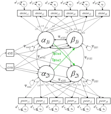
3.3 Multivariate Conditional Linear LCM with Two TICs and Two Sets of Repeated Measures . . . 42
3.3.1 Checks for Model Equivalency . . . 42
3.3.2 Parameter and Standard Error Transformations . . . 44
3.3.3 Empirical Results . . . 45
3.4 Model 4: Conditional TVC LCM with 2 TICs and one set of TVCs . . . 45
3.4.1 Checks for Model Equivalency . . . 48
3.4.2 Parameter and Standard Error Transformations . . . 48
3.4.3 Empirical Results . . . 49
3.5 Model 5: Conditional LCM with 2 TICs and a Distal Outcome . . . 49
3.5.1 Checks for Model Equivalency . . . 52
3.5.2 Parameter and Standard Error Transformations . . . 52
3.5.3 Empirical Results . . . 53
4 Discussion . . . 57
4.1 Analytical Discussion . . . 57
4.1.1 Equivalent Model Rules . . . 57
4.1.2 Parameter Transformations . . . 59
4.1.3 Standard Error Transformations . . . 65
4.2.1 Consequences in Applied Research . . . 67
4.2.2 Recommendations for Applied Researchers . . . 70
4.3 Limitations and Conclusions . . . 72
5 Appendix . . . 74
LIST OF TABLES
3.1 Parameter Transformations for Model 1: Unconditional LCM . . . 35
3.2 Variance Transformations for Model 1: Unconditional LCM . . . 36
3.3 Empirical Results for Model 1: Unconditional LCM . . . 38
3.4 Parameter Transformations for Model 2: Conditional LCM . . . 40
3.5 Variance Transformations for Model 2: Conditional LCM . . . 41
3.6 Empirical Results for Model 2: Conditional LCM . . . 43
3.7 Parameter Transformations for Model 3: Multivariate LCM . . . 46
3.8 Empirical Results for Model 3: Multivariate LCM . . . 47
3.9 Parameter Transformations for Model 4: Conditional TVC LCM . . . 50
3.10 Empirical Results for Model 4: Conditional TVC LCM . . . 51
3.11 Parameter Transformations for Model 5: Conditional LCM with Distal Outcome . . . 54
3.12 Parameter Transformations for Indirect Effects of Model 5: Conditional LCM with Distal Outcome . . . 55
3.13 Empirical Results for Model 5: Conditional LCM with Distal Outcome . . . 56
5.1 Variance Transformations for Model 3: Multivariate LCM . . . 75
5.2 Variance Transformations for Model 4: Conditional TVC LCM . . . 76
5.3 Variance Transformations for Model 5: Conditional LCM with Distal Out-come . . . 77
LIST OF FIGURES
3.1 Model 1: Unconditional LCM with Model A (solid lines) and Model B (dotted lines) . . . 34 3.2 Model 2: Conditional LCM with Model A (solid lines) and Model B
(dot-ted lines) . . . 39 3.3 Multivariate Conditional LCM: Model A (solid lines) and Model B (dotted
lines) . . . 44 3.4 Model 4: Conditional TVC LCM with Model A (solid lines) and Model B
(dotted lines) . . . 48 3.5 Model 5: Conditional LCM with Distal Outcome with Model A (solid
CHAPTER 1
Introduction
Structural Equation Modeling (SEM), sometimes called Covariance Structure Modeling (CSM), is a statistical technique heavily used in the social sciences. The objective is to understand and evaluate the relations among a set of observed vari-ables and latent (unobserved) varivari-ables. This is accomplished by using a model that is hypothesized to represent the relations among the variables. The covariance struc-ture implied by this model is then reproduced as function of model parameters. The goal is to find parameter values that minimize the discrepancy between the observed covariance matrix and the model implied covariance structure (Bollen, 1989).
1.1 Latent Curve Modeling
1.1.1 Model Properties and Assumptions
Meredith and Tisak (1984, 1990), drawing on work from Rao (1958) and Tucker (1958), first described LCM in the form of a confirmatory Factor Analysis with spe-cific constraints or a highly restricted SEM. These models incorporate a mean struc-ture in addition to the standard covariance strucstruc-ture. For linear models, a major advantage of LCM over more traditional models, such as Repeated Measures Anal-ysis of Variance (ANOVA) or AnalAnal-ysis of Covariance (ANCOVA), is the allowance of individual differences in intercept (initial starting point) and slope (growth over time). Thus, these models may conform more closely to actual patterns in data found in the social sciences. To illustrate model properties, model assumptions, and es-timation procedures, I will describe an unconditional linear LCM. In this model, the latent trajectories are parameterized by a latent intercept factor, reflecting initial starting point, and a latent slope factor, reflecting linear rate of change over time. The repeated measures are a function of the latent factors plus error, as represented by:
yit =αi+λtβi+eit
αi =µα+ζαi
βi =µβ+ζβi
(1.1)
where yit represents the repeated measures for individual i at time point t, αi
rep-resents the latent random intercept, λt contains factor loadings specifying value of
time,βirepresents the latent random slope, andeitrepresent the time and individual
specific errors of the repeated measures. While I am focusing on a linear functional form, note that there are many different functional forms that can be represented in
λt. The latent factors are functions of an overall mean and random effect.
the individual specific deviation from this mean intercept. Similarly, µβ is the mean
of the latent slopes aggregating across individuals and ζβi is the individual specific
deviation from this mean slope. This can be expressed in matrix form:
y =Λ(µη+ζ) +e (1.2)
where y is a vector of repeated measures, Λ is a matrix of factor loadings, µη is a vector of latent factor means, ζ is a vector of latent factor residuals, and e is a vector of residuals of the repeated measures. The elements of the matrices are illustrated as follows:
yi1
yi2
... yiT
=
1 0
1 1
...
1 T−1
µαi
µβi
+
ζαi
ζβi
+
ei1
ei2
...
eiT
whereirepresents individual and T represents total number of time points. The variances and covariances of model parameters are defined by:
var(αi) = ψαα
var(βi) = ψββ
cov(αi,βi) = ψαβ
var(eit) = σt2
with expected values:
E(αi) = µα
E(βi) = µβ
E(ζαi) = 0 E(ζβi) = 0 E(eit) = 0
(1.4)
Thus, these models make the assumptions that there is an overall mean intercept and slope each with a disturbance that has a distribution with a mean of zero and variance of ψαα and ψββ, respectively, and covariance ψαβ. Also, the residual variances of the
repeated measures are assumed to have a mean of zero and to be constant across indi-viduals within a given time point but are allowed to vary over time points, although this assumption can be relaxed by incorporating other error structures. Additional model assumptions are illustrated with the following equations:
cov(eit,ζαi) = 0
cov(eit,ζβi) = 0
cov(ζαi,ζαj) = 0, wherei 6= j cov(ζβi,ζβj) = 0, wherei 6= j
cov(ζαi,ζβj) = 0, wherei 6= j cov(eit,ejt) = 0, wherei 6= j
cov(eit,ej,t+s) = 0, wherei 6= j
(1.5)
individuals are zero, the covariances of the residuals over individuals with a given time point are zero, and the covariances of the residuals across individuals and across time points are zero. See Bollen and Curran (2006) for a more detailed description.
There exists a variety of ways to expand the LCM in order to test a more com-plicated theoretical question. Manipulation of the λt values can allow for different
paramterizations of functional forms, such as nonlinear trajectories, or the specifica-tion of the intercept value at time points other than initial starting point (Biesanz, Deeb-Sossa, Aubrecht, Bollen, & Curran, 2004). There are several different meth-ods available to paramterize nonlinear growth. A method that retains linearity in the parameters involves using a polynomial function (quadratic, cubic, quartic, etc.). Another method retaining linearity with respect to the parameters is referred to as the ”fully latent” model, which freely estimates certain factor loadings, or values of λt, with the intent of more closely capturing the nature of the growth trajectory
(McArdle, 1988, 1989; Meredith & Tisak, 1984, 1990). A piecewise model, or spline model, can also be used, which splits the data at a chosen time point such that one half follows one trajectory and the other follows a distinct trajectory. Models that are nonlinear in the parameters are also available, such as an exponential trajectory or a cyclic function parameterized using a sine or cosine function.
Further model extensions involve the inclusions of covariates, which can enter the model in a number of ways. These include Time Invariant Covariates (TICs) that do not vary as a function of time, such as gender, Time Varying Covariates (TVCs) that are allowed to have different values at differing time points, or covariates that themselves serve as a set of repeated measures leading to the Multivariate LCM.
factors:
αi =µα+γαx1x1i+γαx2x2i+ζαi
βi =µβ+γβx1x1i+γβx2x2i+ζβi
(1.6)
where x1i and x2i are TICs with regression coefficients of γαx1 and γαx2 for the
in-tercept factor and γβx1 and γβx2 for the slope factor. The latent factors are now
endogenous variables with intercepts and variances conditioned on the effects of the TICs.
Adding TVCs requires a modification of (1.1) by including predictors of the re-peated measures:
yit =αi+λtβi+γtzit+eit (1.7)
where zit is the TVC with a regression coefficient of γt that can vary at each time
point. Lagged effects can also be estimated by including the repeated measure of the previous time point, zi,t−1, as a predictor.
The TVCs may have their own trajectory that the TVC model will not explicity model. In this case, a multivariate LCM can be used, which simultaneously estimates two latent trajectories by using two sets of observed repeated measures, and allowing all latent factors to covary (McArdle, 1989). Thus, (1.1) is implemented for both sets of repeated measures, with a covariance matrix for the latent factors. The extent to which the latent trajectories correspond is captured by the covariances between them. It is also common to allow correlated errors within time and across repeated measures. Bollen and Curran (2006) provide a more detailed description of model properties and possible model extensions.
1.1.2 Estimation of LCM
to the observed covariance structure, which serves as an estimate of the population covariance structure. The discrepancy between the model implied and observed co-variance structures is minimized. However, LCMs also incorporate a mean structure, which is obtained by taking the expected values of the model equations. This model implied mean structure is then compared with the observed mean structure, which serves as an estimate of the population mean structure. Taken together, the model implied covariance and mean structures are compared to the observed covariance and mean structures and the discrepancy between them is minimized.
To illustrate estimation procedures, I return to the unconditional linear LCM. The model implied equation for the means of the observed variables is obtained by taking the expected value of the observed variables:
E(yit) =µα+λtµβ (1.8)
which can be expressed in matrix form as:
E(y) = Λµη (1.9)
The model implied equations for the variances and covariances of the observed vari-ables are obtained by taking the variance ofyit and covariances ofyit withyi,t+s. This
can be seen in scalar form:
var(yit) =ψαα+λ2tψββ+2λtψαβ+σt2
cov(yit,yi,t+s) =ψαα+λtλt+sψββ+ (λt+λt+s)ψαβ
(1.10)
and matrix form:
whereΛis defined as before, Ψis a variance-covariance matrix of latent factors:
Ψ=
ψαα ψβα
ψαβ ψββ
and Θe is a diagonal matrix which contains the residual vairances of the observed variables. The elements in these matrices constitute the model parameters.
All of the model parameters are then placed into a vector, θ. The observed mo-ment matrices are then equated to the expected momo-ment matrices:
µ =µ(θ) (1.12)
µy1
µy2
...
µyT
=
µα+λ1µβ
µα+λ2µβ
...
µα+λTµβ
Σ =Σ(θ) (1.13)
var(y1) cov(y1,y2) · · · cov(y1,yT)
cov(y2,y1) var(y2) · · · cov(y2,yT)
... ... . .. ...
cov(yT,y1) cov(yT,y2) · · · var(yT)
=
ψαα+λ21ψββ+σ12 · · · ψαα+λ1λTψββ+ (λ1+λT)ψαβ
ψαα+λ2λ1ψββ+ (λ2+λ1)ψαβ · · · ψαα+λ2λTψββ+ (λ2+λT)ψαβ
... . .. ...
ψαα+λTλ1ψββ+ (λT +λ1)ψαβ · · · ψαα+λ2Tψββ+2λTψαβ+σT2
implied characteristics of the variables. In order to accomplish this, parameter values inθare chosen such that a function that represents the discrepancy between observed and model implied moments is minimized. This function is called a fit function, and when using Maximum Likelihood (ML) estimation is defined as:
FML =ln|Σ(θ)| −ln|S|+tr[Σ−1(θ)S]−p+ [y¯ −µ(θ)]0Σ−1(θ)[y¯ −µ(θ)] (1.14)
whereSis the observed covariance matrix, ¯yis a vector of observed means, and pis the number of observed variables. This function will be zero if there is no discrepancy between the model implied moment matrices and observed moment matrices. The parameter estimates in θ are chosen such that this function is as close to zero as possible.
Other estimators exist, such as unweighted least squares (ULS), weighted least squares (WLS), and generalized least squares (GLS). Bollen (1989) offers a thorough descriptions of these and other estimators. All such estimators share a common objective of minimizing a fit function, the difference is in how the fit function is defined. An advantage of using ML estimation is that, asymptotically, parameter es-timates produced are unbiased, consistent, efficient, and normally distributed. Also, ML estimation can produce inferential tests by computing the standard errors (SE) of parameter estimates. The SEs are obtained from the diagonals of the asymptotic covariance matrix (ACOV) which is computed with the following equation:
ACOV = 2
N−1
(
E
"
∂2FML
∂θ∂θ
0#)−1
(1.15)
SEs of the parameter estimates. With such standard errors, a critical z ratio can now be calculated and a test of the null hypothesis that the population parameter is zero can be performed.
Using ML estimation also allows for the calculation of a chi-square goodness of fit measure as well as a plethora of other fit indexes (Bollen & Curran, 2006; Bollen & Long, 1993). When the fit function is multiplied by (N−1), the result is distributed asχ2with degrees of freedom (d f) equal to the number of observed moments minus the number of estimated parameters:
TML = (N−1)FML ∼χ2 µ
1
2T(T+3)−u
(1.16)
where TML represents the chi-square test statistic, T is the number of observed
zero (Bollen & Curran, 2006). The TLI takes on the form:
TLI = Tb/d fb−Th/d fh
Tb/d fb−1 (1.17)
whereTh and d fh represent the chi-square test statistic and associated d f for the hy-pothesized model andTb andd fb represent the chi-square test statistic and associated d f for the baseline model. Other fit indexes that compare the baseline model to the hypothesized model include the Incremental Fit Index (IFI; Bollen, 1989), the Relative Noncentrality Index (RNI; McDonald & Marsh, 1990), and the Comparative Fit Index (CFI; Bentler, 1990). Other fit indexes have been developed that do not use a baseline model, such as the Root-Mean-Square Error of Approximation (RMSEA; Steiger & Lind, 1980) which is defined as:
RMSEA=
s
Th−d fh
(N−1)d fh (1.18)
Another fit index that does not rely on a baseline model is the Bayesian Information Criterion (BIC; Schwarz, 1978; Raftery, 1993), which is defined as:
BIC =Th−d f ln(N) (1.19)
Despite several differences in form, all such fit indexes rely on the correspondence of the data to the model implied moments. This is illustrated by the fact that, for all equations, the fit index is in part a function of Th. These indexes are often used to
decide whether a model is a valid representation of the data. If values of the indexes indicate good fit, the use of the model is often justified. However, if there are two competing models that have the exact same FML and subsequently the same Th, the
1.2 Equivalent Models
1.2.1 Formal Definition and Analytical Identification
While it is not the case for LCMs, the phenomenon of equivalent models has been extensively investigated within the SEM framework (e.g., Lee & Hershberger, 1990; MacCallum et al., 1993; Raykov & Penev, 1999). An informal definition of an equivalent model is that, given a candidate model M, there exists an equivalent model M0 that, when fit to any set of data, will produce the same model implied covariance matrix. As a result, both models will have the same χ2 goodness of fit
statistic, as this statistic is a function of the differences between the observed and model implied covariance matrices. All other fit indexes, including those described in 1.1.2 will also be the same, provided that the same baseline model is used when applicable.
A more formal definition of model equivalence is given by Raykov and Penev (1999), who developed an analytical rule for identifying equivalent models that is both necessary and sufficient. They define Model M and Model M’ as two models with parameter spacesΘ andΘ0, respectively. They state that a transformation func-tion g : Θ → Θ0 exists if for every elementθ in Θ there exists a θ0 in Θ0 such that g transforms θ into θ0 (i.e. θ0 = g(θ)). This means that for every parameter in M there is a function that maps this parameter onto a parameter in M0. If this function exists, what Raykov and Penev define as the Σ-condition is satisfied. More specifically, the Σ-condition is satisfied if for all θ in Θ and corresponding model implied matrices Σ(θ) and Σ(θ0), the transformation function mapsΣ(θ) ontoΣ(θ0). They next define
that a surjective transformation exists if for every element θ0 in Θ0 there exists a θ
Raykov and Penev (1999) provide the following proposition:
Proposition 1: Two models M and M0 are equivalent if and only if they fulfill theΣ-condition with a surjective transformationg : Θ→Θ0relating their parameter spaces. (p.206)
1.2.2 Model Equivalency Identification Rules
While the rule for identifying equivalent models described by Raykov and Penev (1999) is necessary and sufficient, it can be extremely time consuming and compu-tationally intensive to identify all equivalent models that exist for a given model. Several rules have been developed that are easy to implement and can serve as a guide for identifying equivalent models. After such equivalent models are identi-fied, the rule described by Raykov and Penev (1999) can be applied to formally test for model equivalence. Such empirical rules for identifying equivalent models have been described by Stelzl (1986), Lee and Hershberger (1990) and Hershberger (2006). The rules developed by Lee and Hershberger (1990) and extensions of these rules de-scribed by Hershberger (2006) subsume the previous set of rules developed by Stelzl (1986). Thus, I will discuss the more recent rules in detail.
Lee and Hershberger (1990) proposed a rule for identifying equivalent models which they termed the ”replacing rule”. This rule applies to the structural (relations among latent variables and/or observed variables) part of a model, while treating the measurement model as ’fixed.’ It does not matter if the variables are observed or latent, only that they are part of the structural model. To implement this rule, the candidate model is separated into three blocks: a preceding block (PBL), a focal block (FBL), and a succeeding block (SBL). The relations within and between blocks must exhibit ’limited block-recursiveness’ which means that non-recursive relations are allowed within the PBL and succeeding block. However, relations between all blocks and within the FBL must be recursive. The FBL is where the modification of paths will take place, the PBL contains variables that predict those in the FBL, and the SBL contains variables that are causes of those in the FBL.
1. If a FBL exists with source variable x and effect variable y (i.e. x → y), then this direct path can be replaced by a residual covariance if and only if the effect variable, y, has the same or includes all predictors (in the PBL) of the source variable, x.
2. If a FBL exists with a residual correlation between two variables (r(x) ↔r(y)), the correlation can be replaced by a direct path if and only if, in the resulting model, the new effect variable, yhas the same or includes all predictors (in the PBL) of the new source variable, x.
3. If the source and effect variables in a FBL have the same predictors in the PBL, then the relation between the source and effect variables can be a residual cor-relation, a direct relation of source predicting effect, or a direct relation of effect predicting source. This is called a ’symmetric FBL.’
4. If a PBL is saturated or just-identified (that is, every variable in the block is related to every other variable with either a direct structural path or a non-directional covariance), any restructuring of the candidate PBL that produces another just-identified PBL will result in an equivalent model. In this sense, a just-identified PBL is now a FBL.
Hershberger (2006) explains even more variations of rules that can be extended from the replacing rule. He specifies a special case of the replacing rule that allows for a non-recursive path to exist between two variables in the FBL. In this case, the FBL must be a symmetric FBL and the two directed paths of the non-recursive path must be constrained to be equal. If this holds true, then the non-recursive path may be replaced by a directed path (in either direction) or a residual covariance. Hershberger also explains that, within a symmetric FBL, a directed path or residual covariance can be replaced by a non-recursive path that is constrained to be equal. Hershberger also describes a rule for generating equivalent models in the context of measurement models, which he calls the ”reversed indicator rule”. He first states that, given two highly correlated indicators, there exists a greater chance of there being a large number of equivalent models as there can be many ways this large correlation can be captured. The reversed indicator rule states that: For a given measurement model, the causal direction of a path between just one indicator and a latent variable can be reversed or replaced by an equated nonrecursive path if a) the measurement model is exogenous or has only one indicator before and after the rule is applied and b) the exogenous latent variable is uncorrelated with other exogenous latent variables before and after the rule is applied.
1.2.3 Prevalence and Consequences
- 1987. Of these, he found only one that mentioned the existence of an alternative equivalent model. He also noted that, in most cases, there were many such equiv-alent models that the authors failed to acknowledge. Furthermore, some of these equivalent models provide plausible and meaningful interpretations of the research question, sometimes even contradicting the conclusions of the original model.
MacCallum et al. (1993) examined instances of SEM during the period from 1988 - 1991 from three journals (Journal of Educational Psychology, Journal of Applied Psychology, Journal of Personality and Social Psychology). They found a total of 99 applications of CSM, none of which mentioned the existence of an equivalent model. They also found that 90% of the cases had at least one equivalent model and half had 16 or more equivalent models. This suggests that equivalent models are common in psychological research, often in large numbers. A more recent study by Roesch (1999) examined 50 instances of SEM from a large variety of behavioral science journals ranging from the years 1984 to 1995. Of these, only one mentioned the existence of an equivalent model (this is the same one from MacCallum et al., 1993).
the-oretical hypothesis. For the second and third equivalent models, the authors provide meaningful interpretations that seem to be just as plausible as the interpretation of the original model. Thus, each of the four models provides a different substantive understanding of the relations of variables while generating the exact same model fit. Ignoring the existence of these other plausible models may seriously distort and inflate the confidence one places in the original model. If it seems that the model fits the data fairly well, and the patterns of relations among variables corresponds with prior theory, then one may falsely conclude that this model is ’correct’ and rule out or fail to consider other theories.
Another important reason for studying equivalent models is described by Hershberger (2006). He states that, when testing a model, we are really testing a whole set of models that are statistically indistinguishable from the candidate model. This can lead to falsely accepting a model that is statistically indistinguishable from the ’true’ model. If the equivalent models are ignored, it is thus possible that the conclusions are spurious. In applications of LCMs, these same principles hold. Thus, without adequately studying this problem, it is possible that many applications are partially, if not wholly, incorrect.
1.3 Equivalent Models as Related to LCM
LCMs, however, an informal literature review I conducted reveals that they do not discuss the idea of equivalent models. I searched for recent LCM applications, and found that none mentioned the problem of equivalent models or cited any of the seminal articles on equivalent models. This can lead to a false sense of confidence in the author’s model of choice, as it is possible that there exists a collection of equiv-alent models that exhibit different substantive interpretations. This problem alone warrants further investigation of the topic.
Since the equivalent model problem has been assessed within the SEM frame-work, it might seem that all possible extensions could apply to the LCM. However, there are also several distinct features of LCMs that are not present in a standard SEM, and it is not clear whether previous findings will extend to LCMs. First, LCMs incorporate a mean structure as well as a covariance structure. Previous examinia-tions of model equivalency have focused solely on covariance structure equivalence, with the exception of Levy and Hancock (2007). However, they did not focus specifi-cally on equivalent models in LCMs, instead focusing on models with a mean struc-ture that are only partially equivalent. It is thus not clear whether such findings extend to LCMs. Second, LCMs incorporate a highly restricted factor loading, or Λ, matrix. While the replacing rule treats the measurement model as fixed, it is assum-ing a more traditional measurement model. So, it is unclear whether a model with a highly restricted measurement model will require a modification of equivalent model rules. One goal of this manuscript is to determine whether previous findings hold for LCMs.
pronounced. For example, if the rescaling of a parameter estimate in an equivalent model is a function of the parameter estimate divided by the variance of the inter-cept, then as the variance of the intercept becomes larger this parameter estimate will go to zero. In this case, under such a condition of a large intercept variance, it may be more likely for a significant effect to vanish upon equivalent respecification. This is just one example, and there may also be conditions under which non-significant effects become significant. Understanding what these exact conditions are will help to illuminate the equivalent model problem and provide insights for choosing ulti-mate models. One goal of this manuscript is to analytically determine parameter rescalings for common LCMs and evaluate consequences of such rescalings.
However, it is also essential to understand the rescalings of standard errors as well as parameter estimates. While it is implied in prior research on equivalent models that standard errors are rescaled non-proportionally to parameter estimates, it is not known how these rescalings are computed or what elements make up the functions of these rescalings. Much focus has been on parameter estimates increasing or decreasing in magnitude, but for overall interpretation purposes, it may not matter that a parameter estimate is doubled in absolute magnitude if the standard error is tripled in magnitude, thus making the overall effect non-significant. One goal of this manuscript is to determine a method for rescaling standard errors and subsequently evaluate how standard errors and overall significance levels are being rescaled in common LCMs.
A final, but important, reason for studying equivalent models in the context of LCMs is that researchers often posit theories that require a reparameterization of standard LCMs. For example, a common reparameterization is to regress the slope factor on the intercept factor, as opposed to allowing for a non-directional covari-ance. This strategy has been implemented in Multivariate LCMs. For example, Curran, Stice, and Chassin (1997) hypothesize a model where the slope from one set of repeated measures is regressed upon the intercept for the other set of repeated measures, and vice versa. A more recent application by Tildesley and Andrews (2008) employed similar models where the intercept of parent alcohol use predicted the in-tercept and slope of child alcohol intentions, and the slope of parent alcohol use predicted the slope of child alcohol intentions. Also, B. O. Muth´en and Curran (1997) suggest a model where slopes and intercepts of one growth process predicts slopes and intercepts of another growth process. They also suggest a model where an in-tercept factor predicts a second slope growth factor, while retaining the standard covariance between the intercept factor and first slope factor. In substance use lit-erature, the idea that initial status predicts growth over time has been hypothesized (Zucker, 2006; Chassin, Hussong, & Beltran, in press). It is thus of theoretical inter-est to tinter-est whether intercept, parameterized as an individual’s initial starting point, predicts an individual’s growth trajectory. This reparameterization requires a direct relation from intercept to slope substituting the non-directional covariance. Such a reparameterization may result in an equivalent models with identical fit, however, the substantive interpretation is different and parameter estimates are rescaled.
CHAPTER 2
Methods
To achieve the goals of this study, I performed an analytical and empirical analy-sis for a set of common LCMs. Prior to analyanaly-sis, I selected a set of candidate models and a reparameterization of each candidate model into an equivalent model. Next I implemented a three-staged strategy for analysis. For each pair of models I analyt-ically computed the parameter transformations, analytanalyt-ically computed the standard error transformations, and empirically analyzed an existing data set using both candi-date and equivalent models. Accordingly, this section will first describe the methods for model selection, followed by a description of methods for the analytical deriva-tions of parameter estimate and standard error transformaderiva-tions, concluding with a description of the empirical analyses.
2.1 Model Selection
All models have six time points in order to conform to subsequent empirical data. Also, all models have a linear functional form and estimate a random intercept and random slope parameter. The candidate models are as follows:
1. Unconditional linear LCM
2. Conditional linear LCM with 2 TICs
3. Multivariate Conditional linear LCM with 2 TICs and 2 sets of repeated mea-sures
4. Conditional TVC linear LCM with 2 TICs and one set of TVCs
5. Conditional linear LCM with 2 TICs and a Distal Outcome
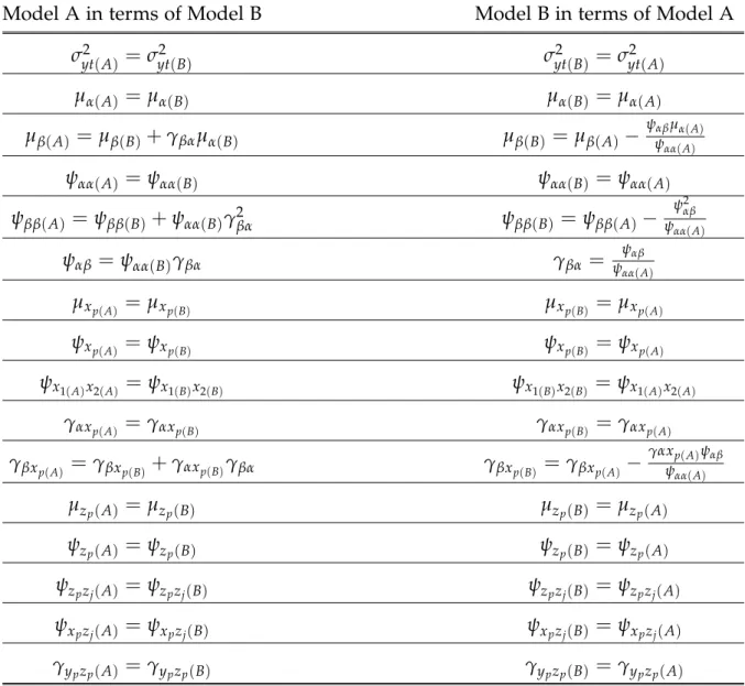
I re-parameterized each candidate model into an equivalent model. Throughout this manuscript, Model A will refer to the candidate model and Model B will refer to its respective equivalent model. For all models except the Multivariate Conditional LCM, the re-parameterization is allowing slope to be regressed upon intercept. As this structure of initial starting point predicting rate of change has been hypothesized in literature for substance use research (Zucker, 2006; Chassin et al., in press), it substantively serves as a viable model. For the Multivariate Conditional LCM, the slope from the first set of repeated measures is regressed upon the intercept from the second set of repeated measures, and the slope of the second set of repeated measures is regressed upon the intercept from the first set of repeated measures. This serves to replicate a model hypothesized by McArdle (1989) and used in subsequent substantive applications (Curran et al., 1997).
2.2 Analytical Examination of Parameter Transformations
context and to determine prevalence of equivalent models in LCMs. I applied the analytical rules described by Raykov and Penev (1999) to obtain transformations of parameter estimates. In order to accomplish this, I solved for the model implied mean structure and model implied covariance structure for each model. I then stacked the non-redundant elements of these matrices into a vector for Model A and Model B. I then equated these vectors and solved as a system of simultaneous equations for the parameters in Model A in terms of Model B, and again for the parameters in Model B in terms of Model A.
Solving for the model implied moment structures can be done equation by equa-tion with expectaequa-tion rules and variance and covariance rules. However, this can be tedious and error prone. I thus computed these model implied moment structures using a general matrix formulation. Specifically, the covariance and mean structure are generated using the general matrix expression described by Bollen and Curran (2004). This matrix structure was used because it allows for the specification of all equivalent models with a small number of matrices, thus providing a flexible and parsimonious method for computing the moment structures. Five matrices are cre-ated to capture the parameterization of each model. The first represents the means of the variables:
µ =
µy
µz
µα
µβ
depending on the parameterization of the model.
The next matrix represents the structural relations among variables:
B=
Byy Byz Byα Byβ
Bzy Bzz Bzα Bzβ
Bαy Bαz Bαα Bαβ
Bβy Bβz Bβα Bββ
whereByy represents the structural relation of the variables in yregressed upon the variables in y, Byz represents the structural relation of the variables in y regressed upon the variables in z, and so forth. This matrix can be further broken down into:
B=
By1y1 · · · By1yp
... . .. ...
Bypy1 · · · Bypyp
By1z1 · · · By1zq
... . .. ...
Bypz1 · · · Bypzq
By1α
... Bypα
By1β
... Bypβ
Bz1y1 · · · Bz1yp
... . .. ...
Bzpy1 · · · Bzqyp
Bz1z1 · · · Bz1zq
... . .. ...
Bzqz1 · · · Bzqzq
Bz1α
... Bzqα
Bz1β
... Bzqβ
Bαy1 · · · Bαyp
Bβy1 · · · Bβyp
Bαz1 · · · Bαzq
Bβz1 · · · Bβzq
Bαα Bβα Bαβ Bββ
this framework is flexible enough to allow for all possible structural relations in all candidate and respective equivalent models. Accordingly, this achieves the ultimate goal of having a parsimonious method for computing the model implied moment structures.
The next symmetric matrix parameterizes the covariances among all variables:
Σ =
var(y1)
... . ..
cov(y1,yp) · · · var(yp)
cov(y1,z1) · · · cov(yp,z1) var(z1)
... . .. ... . ..
cov(y1,zq) · · · cov(yp,zq) cov(z1,zq) var(zq)
cov(y1,α) · · · cov(yp,α) cov(z1,α) · · · cov(zq,α) var(α)
cov(y1,β) · · · cov(yp,β) cov(z1,β) · · · cov(zq,β) cov(αβ) var(β)
Any covariances not specified in a given model are given a value of zero, and any covariances that are specified are allowed to be freely estimated.
A final matrix serves to pick out the observed variables via Identity matrices:
P =
Ip 0 0 0
0 Iq 0 0
where Ip is the Identity matrix of dimension pxp and Iq is the Identity matrix of
dimension qxq.
The model implied mean vector is computed from:
The model implied covariance matrix is computed from:
Σ(θ) = P(I−B)−1Σ(I−B)−10P0 (2.2)
where ’ is the usual transpose operation.
I used Mathematica version 6 to compute the model implied mean and covariance structures for each candidate and equivalent model. For each candidate model, all non-redundant elements are stacked into a vector. All non-redundant elements of the corresponding equivalent model are stacked into a different vector. These vectors are equated and solved as a set of simultaneous equations. The parameters of the Model A are solved for in terms of parameters in Model B and then the parameters in Model B are solved for in terms of parameters in Model A.
2.3 Analytical Examination of Standard Error Transformations
I used the Multivariate Delta Method (Bishop, Fienberg, & Holland, 1975) to obtain the rescalings of standard errors. This method obtains approximate stan-dard errors given the transformation function is ”smooth.” Since such transformation functions are sums, differences, products, and ratios of parameter estimates, the func-tions are continuous and do not abruptly change direction, and thus are considered ”smooth functions” (Raykov & Marcoulides, 2004).
A first-order Taylor series approximation is used where parameter estimates serve as variables. Raykov and Marcoulides (2004) note that higher-order approx-imations do not provide a significant amount of additional information, thus I only considered first-order approximations.
approximation is:
f(θˆ1, ˆθ2, . . . , ˆθp) ≈ f(θ10,θ20, . . . ,θp0) +D1(θˆ1−θ10) +D2(θˆ2−θ20) +. . .+Dp(θˆp−θp0).
(2.3) where
Dj =
∂f(θ10,θ20, . . . ,θp0)
∂θj . (2.4)
and θ0 = population value of θ. Since the population values of parameter estimates
are considered to be the estimates themselves, the new parameter is simply the func-tion itself. The approximate variance associated with this funcfunc-tion is:
ˆ
σ2(f) ≈D2
1σ2(θˆ1) +D22σ2(θˆ2) +. . .+D2p(σˆp) +2D1D2σ(θˆ1, ˆθ2) +
2D2D3σ(θˆ2, ˆθ3) +. . .+2Dp−1Dpσ(θpˆ−1, ˆθp). (2.5)
whereσp2(θˆp)is the asymptotic variance of the pthparameter estimate andσ(θˆp−1, ˆθp)
is the asymptotic covariance of the p−1 and pth parameter estimates. A matrix expression for transformations of variances is:
σ2(f)≈ ∂f(θ)
∂θˆ0 ACOV[θ]ˆ
∂f(θ)
∂θˆ (2.6)
where ∂f(θ)
∂θˆ0 is a first-order partial derivative matrix of parameter transformation
2.4 Empirical Applications
2.4.1 Sample and Participants
For each candidate and equivalent model, I analyzed data from the Adolescent and Family Development Project (Chassin, Rogosch, & Barrera, 1991). In this study, adolescents and their parents participated in a longitudinal study on adolescent sub-stance use. Adolescents were either children of alcoholics (COAs; n = 246), meaning they had at least one biological and custodial alcoholic parent, or controls (n = 208), meaning neither parent was an alcoholic . A total of 454 participants were recruited and interviewed five times (see Chassin, Barrera, Bech, & Kossak-Fuller, 1992 for details on recruitment procedures). In order to correspond more closely to analyses conducted by Curran et al. (1997), the first three time points were used. In accordance with Curran et al. (1997), 74 individuals were dropped from analyses as they reported no use over time on both the alcohol use and peer use variables. An additional 5 in-dividuals were dropped as they displayed an abberrant trend in drinking behavior. Participants were aged 10 to 16 at Time 1, 11 to 17 at Time 2, and 12 to 18 at Time 3. So as not to confound wave of assessment and age of adolescents, participants were rearranged by age instead of wave (Mehta & West, 2000). Thus, participant ages ranged from 10 to 18. However, due to spareness of both participants and response frequencies at the earlier and later ages, this study included participants aged 12 to 17, for a total of 6 time points. Final analyses had a total sample size ofN =373 with missingness by design and attrition. Specifically, four adolescents only have data for Wave 1, one adolescent has data for Wave 1 and Wave 3, and five adolsecents only have data for Wave 1 and Wave 2.
2.4.2 Measures
use in the past 12 months using a scale from 0 (not at all) to 7 (every day). The questions asked about frequency of consumption of beer, wine, and hard liquor (two items), consumption of five or more drinks in a row (one item), and frequency of getting drunk (one item). These variables were summed at each time point to arrive at an summed score measure of adolescent alcohol use. Adolescent alcohol use was calculated in the same manner for Wave 5 alcohol use, which served as the distal outcome.
Peer alcohol use. Peer alcohol use was operationalized by two variables at each time point. Adolescents were asked two questions concerning alcohol consumption of their peers. Adolescents were asked to rate, on a scale from 0 (none) to 5 (all), how many of their friends drank occasionally and how many of their friends drank regularly. The two items were added to produce a summed score measure of peer alcohol use.
Externalizing Symptomatology. At Time 1, each child’s degree of externalizing symptomatology was assessed using child reports from the Child Behavior Checklist (Achenbach & Edelbrock, 1981). A subset of 21 items were used with an expansion of the response scale to 5 to increase variance. Higher values are indicative of lower externalizing symptomatology.
Parent alcoholism A dichotomous variable specifying whether children had an alcoholic parent (COA; Child of Alcoholic) was coded (presence, coded 1; absence, coded 0) with information from a computerized version of the Diagnostic Interview Schedule (DIS, Version III; Robins, Helzer, Croughan, & Ratcliff, 1981).
2.4.3 Analysis Details
CHAPTER 3
Results
For each pair of models, I present results containing checks for model equiva-lency, parameter and standard error transformations, and empirical findings. Param-eter and standard error transformations for the unconditional LCM were checked by hand and with the empirical results. All other transformations were checked with the empirical results. Table 5.4 in Appendix 5 contains the actual and derived variance values for the multivariate LCM. The tables containing parameter transformations include a column of tranformations of paramters in Model A in terms of parameters in Model B followed by a column of transformations of parameters in Model B in terms of parameters in Model A. Tables containing standard error transformations include only those transformations that are not an indentity transformation for each parameter in Model B as a function of parameters in Model A. The rescalings of the variances are displayed for ease of presentation, as the standard error is simply the square root of the variance.
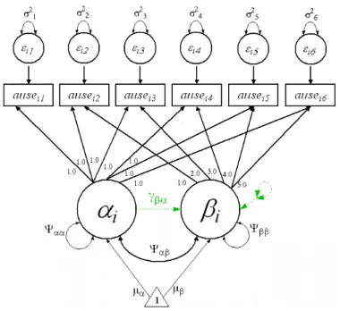
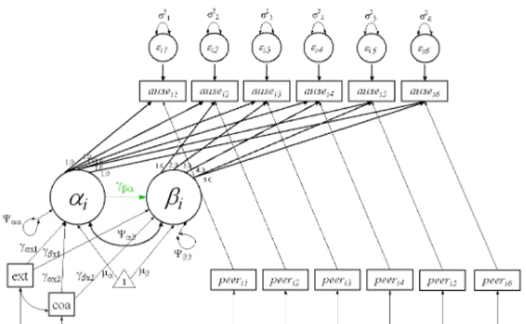
3.1 Model 1: Unconditional LCM
Figure 3.1: Model 1: Unconditional LCM with Model A (solid lines) and Model B (dotted lines)
3.1.1 Checks for Model Equivalency
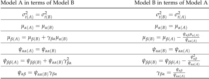
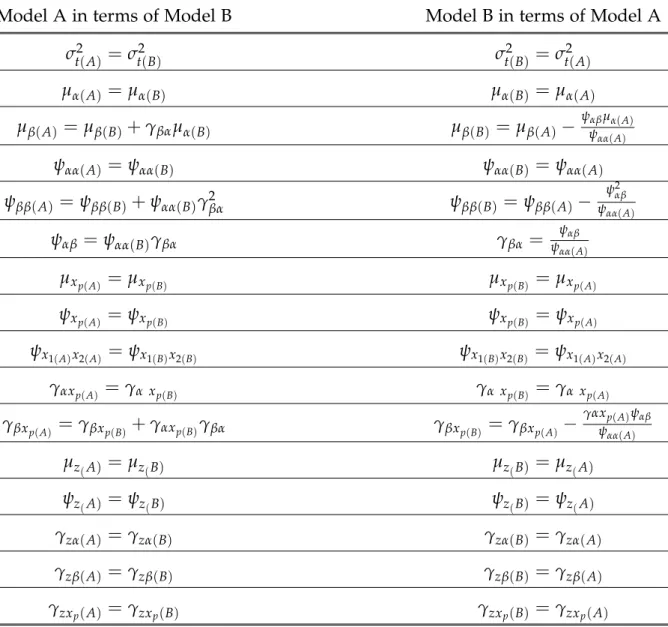
Table 3.1: Parameter Transformations for Model 1: Unconditional LCM
Model A in terms of Model B Model B in terms of Model A
σt2(A) =σt2(B) σt2(B) =σt2(A)
µα(A) =µα(B) µα(B) =µα(A)
µβ(A) =µβ(B)+γβαµα(B) µβ(B) =µβ(A)−
ψαβµα(A)
ψαα(A)
ψαα(A) =ψαα(B) ψαα(B) =ψαα(A)
ψββ(A) =ψββ(B)+ψαα(B)γ2
βα ψββ(B) =ψββ(A)−
ψ2
αβ
ψαα(A)
ψαβ =ψαα(B)γβα γβα= ψαβ
ψαα(A)
3.1.2 Parameter and Standard Error Transformations
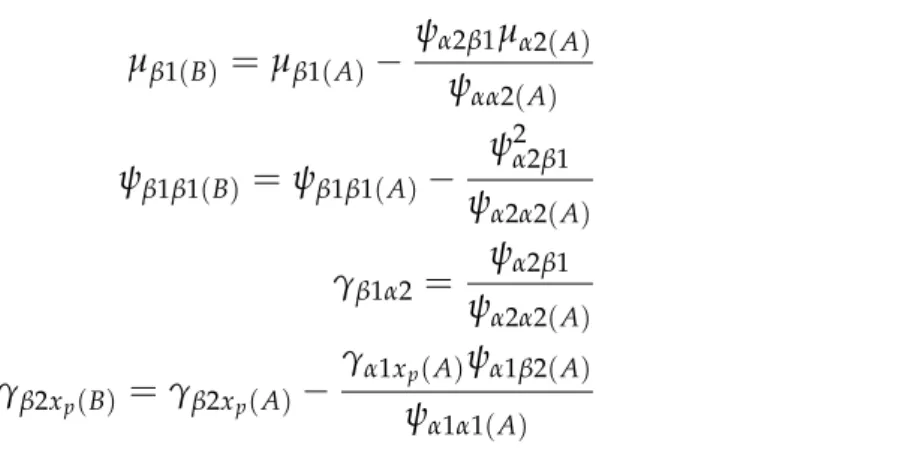
Table 3.1 contains the transformations of parameter estimates for Model A (slope correlated with intercept) and Model B (slope regressed on intercept). Three trans-formations are not the identity transformation: µβ, ψββ, and ψαβ. Specifically, these
parameters have the following transformations of the parameter in Model B in terms of parameters in Model A:
µβ(B) =µβ(A)− ψαβµα(A)
ψαα(A) (3.1)
ψββ(B) =ψββ(A)− ψ
2 αβ
ψαα(A) (3.2)
γβα=
ψαβ
ψαα(A) (3.3)
Table 3.2: V ariance Transfor mations for Model 1: Unconditional LCM Parameter fr om Model B Transfor mation in ter ms of Model A Parameters µβ ( B )
1 4ψαα
(
2
ψ
2 ψαα
α β µα co v ( µα , ψα β ) − 2 ψ
3 αα
ψα β co v ( µβ , ψα β ) + 2 ψ
2 αα
ψα β µα co v ( µβ , ψα α ) − 2 ψ
3 µαα
α co v ( µβ , ψα β ) + 2 ψ
2 ψαα
α β µα co v ( µβ , ψα α ) − 2 ψα α ψα β µ
2 coα
v ( ψα α ψα β )+ ψ
2 αα
µ
2 vα
ar ( ψα β ) + ψ
2 αα
ψ
2 αβ
v ar ( µα ) + ψ
4 vαα
ar ( µβ ) + ψ
2 αβ
µ
2 vα
ar ( ψα α )) γβ α
1 4ψαα
( − 2 ψα α ψα β co v ( ψα α , ψα β ) + ψ
2 αα
v ar ( ψα β ) + ψ
2 αβ
v ar ( ψα α )) ψβ β ( B )
1 4ψαα
(
−
4
ψ
3 αα
ψα β co v ( ψα β , ψβ β ) − 4 ψα α ψ
3 αβ
co v ( ψα α ψα β )+ 2 ψ
2 αα
ψ
2 αβ
co v ( ψα α , ψβ β ) + 4 ψ
2 αα
ψ
2 αβ
v ar ( ψα β ) + ψ
4 αβ
v ar ( ψα α ) + ψ
4 αα
3.1.3 Empirical Results
Both Model A and Model B have identical overall fit and thus identical likeli-hoods with fit indices of χ2(13) =41.379,p =0.0001,RMSEA = 0.077,TLI =0.918. All estimates, standard errors, and significance estimates are provided in Table 3.3. These values correspond to the analytical transformations. Specifically, given rameter values and, in the case of standard errors, variances and covariances of pa-rameters, the analytical transformations can be used to go from one model to the other. Parameters with a non-identity transformation display different estimates, standard errors, and critical ratios in Model A and Model B. For example, the mean slope parameter in Model A is significantly different than zero ( ˆµβ(A) = 0.87,se =
0.09,p < 0.001). The corresponding parameter in Model B, now a conditional mean slope, is also significant but has a larger parameter estimate and standard error ( ˆµβ(B) =0.90,se =0.20,p<0.001). The variance of the slope parameter in Model A is significantly different than zero ( ˆψββ(A) =1.68,se =0.23,p<0.001). The correspond-ing parameter in Model B, now a conditional variance in slope, is significant with a smaller parameter estimate and standard error ( ˆψββ(B) = 1.68,se = 0.26,p < 0.001). The covariance of slope with intercept in Model A is negative and nonsignificant ( ˆψαβ = −0.05,se = 0.36,p = 0.89), while the corresponding parameter in Model B, now a regression coefficient of slope regressed on intercept, is negative and non-significant ( ˆγβα =−0.06,se =0.41,p=0.88).
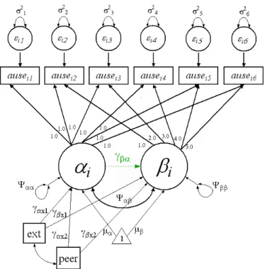
3.2 Model 2: Conditional LCM with Two TICs
Table
3.3:
Empirical
Results
for
Model
1:
Unconditional
LCM
Parameter
Model
A
Model
B
Estimate
SE
Est./SE
p-v
alue
Estimate
SE
Est./SE
p-v
alue
µα
0.463
0.090
5.171
<
0.001
0.463
0.090
5.171
<
0.001
µ β
0.868
0.087
10.032
<
0.001
0.896
0.203
4.418
<
0.001
ψα
α
0.813
0.526
1.547
0.122
0.813
0.526
1.545
0.122
ψα
β
-0.049
0.359
-0.136
0.892
-γβ
α
--0.059
0.408
-0.145
0.884
ψβ
β
1.682
0.288
5.840
<
0.001
1.679
0.259
6.486
<
0.001
Notes
.
1.
Ro
ws
in
bold
repr
esent
p
arameters
that
dif
fer
betw
een
Model
A
and
Model
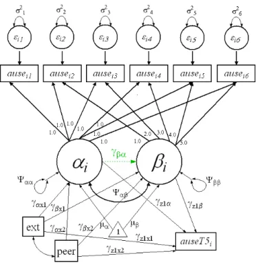
Figure 3.2: Model 2: Conditional LCM with Model A (solid lines) and Model B (dotted lines)
3.2.1 Checks for Model Equivalency
Administering the replacing rule allows for the two latent factors and two TICs to be treated as a saturated PBL. Thus, any modification to a path, be it a non-directional, non-directional, or equated non-recursive path, will result in an equivalent model. Again, these respecifications are independent of the measurement model. A total of 4(42) = 46 or 4, 098 different equivalent models are possible, irrespective of
possible equivalent models produced by modifying values in Λ. 3.2.2 Parameter and Standard Error Transformations
Table 3.4 contains the transformations of parameter estimates for Model A (slope correlated with intercept) and Model B (slope regressed on intercept). Five transfor-mations are not the trivial identity transformation: µβ, ψββ, ψαβ (γβα in Model B),
Table 3.4: Parameter Transformations for Model 2: Conditional LCM
Model A in terms of Model B Model B in terms of Model A
σt2(A) =σt2(B) σt2(B) =σt2(A)
µα(A) =µα(B) µα(B) =µα(A)
µβ(A) =µβ(B)+γβαµα(B) µβ(B) =µβ(A)−
ψαβµα(A)
ψαα(A)
ψαα(A) =ψαα(B) ψαα(B) =ψαα(A)
ψββ(A) =ψββ(B)+ψαα(B)γ2
βα ψββ(B) =ψββ(A)−
ψ2
αβ
ψαα(A)
ψαβ =ψαα(B)γβα γβα= ψαβ
ψαα(A)
µxp(A) =µxp(B) µxp(B) =µxp(A)
ψxp(A) =ψxp(B) ψxp(B) =ψxp(A)
ψx1(A)x2(A) =ψx1(B)x2(B) ψx1(B)x2(B) =ψx1(A)x2(A)
γαxp(A) =γα xp(B) γα xp(B) =γα xp(A)
γβxp(A) =γβxp(B)+γαxp(B)γβα γβxp(B) =γβxp(A) −
γαxp(A)ψαβ
ψαα(A)
represents a TIC). The transformations forµβ, ψββ, andψαβ are the same as found in
Model 1. The transformation of slope regressed on a given TIC is:
γβxp(B) =γβxp(A) −
γαxp(A)ψαβ
ψαα(A) (3.4)
Table 3.5: V ariance Transfor mations for Model 2: Conditional LCM Parameter fr om Model B Transfor mation in ter ms of Model A Parameters µβ ( B )
1 4ψαα
(
2
ψ
2 αα
ψα β µα co v ( µα , ψα β ) − 2 ψ
3 ψαα
α β co v ( µβ , ψα β ) + 2 ψ
2 ψαα
α β µα co v ( µβ , ψα α ) − 2 ψ
3 µαα
α co v ( µβ , ψα β ) + 2 ψ
2 αα
ψα β µα co v ( µβ , ψα α ) − 2 ψα α ψα β µ
2 coα
v ( ψα α ψα β )+ ψ
2 µαα
2 vα
ar ( ψα β ) + ψ
2 ψαα
2 αβ
v ar ( µα ) + ψ
4 vαα
ar ( µβ ) + ψ
2 αβ
µ
2 vα
ar ( ψα α )) γβ α
1 4ψαα
( − 2 ψα α ψα β co v ( ψα α , ψα β ) + ψ
2 vαα
ar ( ψα β ) + ψ
2 αβ
v ar ( ψα α )) ψβ β ( B )
1 4ψαα
(
−
4
ψ
3 ψαα
α β co v ( ψα β , ψβ β ) − 4 ψα α ψ
3 αβ
co v ( ψα α ψα β )+ 2 ψ
2 ψαα
2 αβ
co v ( ψα α , ψβ β ) + 4 ψ
2 ψαα
2 αβ
v ar ( ψα β ) + ψ
4 αβ
v ar ( ψα α ) + ψ
4 αα
v ar ( ψβ β )) γβ xp ( B )
1 4ψαα
(
−
2
ψ
3 ψαα
α β co v ( γα xp , γβ xp ) + 2 ψ
2 γαα
α xp ψα β co v ( γα xp , ψα β ) − 2 ψα α γα xp ψα β co v ( γβ xp ψα α ) − 2 ψ
3 αα
γα xp co v ( γ β xp , ψα β ) + 2 ψ
2 γαα
α xp ψα β co v ( γβ xp , ψα α ) − 2 ψα α γ
2 αx
p ψα β co v ( ψα α , ψα β ) + ψ
2 ψαα
α β v ar ( γα xp ) + ψ
4 vαα
ar ( γβ xp ) + ψ
2 αα
γ
2 αx
p v ar ( ψα β ) + γ
2 αx
p
ψ
2 αβ