Richardson_unc_0153D_15005.pdf

HOW DO CHANGES IN THE NEIGHBORHOOD FOOD ENVIRONMENT INFLUENCE DIET AND BODY MASS INDEX OVER TIME? AN INNOVATIVE METHOD USING 20

YEARS OF SPATIAL, DIET, AND ANTHROPOMETRY DATA

Andrea S Richardson

A dissertation submitted to the faculty at the University of North Carolina at Chapel Hill in partial fulfillment of the requirements for the degree of Doctor of Philosophy in the Department

of Nutrition in the Gillings School of Global Public Health.

Chapel Hill 2014

Approved by:

Penny Gordon-Larsen

Barry M Popkin

Kelly R Evenson

Katie A Meyer

ABSTRACT

Andrea S Richardson: How do changes in the neighborhood food environment influence diet and body mass index over time? An innovative method using 20 years of spatial, diet, and

anthropometry data

(Under the direction of Penny Gordon-Larsen)

Cross-sectional studies suggest neighborhood socioeconomic disadvantage is associated

with obesogenic food environments. Yet, it is unknown how exposure to neighborhood

socioeconomics (SES) patterning through adulthood corresponds to food environments that also

change over time. Further, obesity reduction strategies often target neighborhood food

resources, without considering separate pathways from multiple types of resources to body mass

index (BMI), through diet, or how reverse causality plays a role.

We capitalized on a large Geographic Information Systems derived temporally and

spatially linked to respondents (residential locations) in the large cardiovascular cohort study

called Coronary Artery Risk Development in Young Adults (CARDIA). We estimated longitudinal pathways from neighborhood food resources to BMI and studied pathways from

neighborhood fast food, sit-down restaurants, supermarkets and convenience stores to BMI,

through diet behaviors. We approximated reverse causality with reverse pathways from

period-specific diet behaviors to future neighborhood food resources.

Socioeconomically disadvantaged neighborhood residents had fewer sit-down

restaurants, more convenience stores, and similar numbers of supermarkets in their

were associated with higher BMI through the consumption of foods typically purchased from

fast food restaurants (i.e., fast food-type diet). Fast food-type diet was consistently associated

with higher BMI while consumption of the sit-down restaurant-type diet was associated with

lower BMI. Including reverse pathways from time period specific diet behaviors to future food

environment suggests that diet behaviors may act as a proxy for individual

preferences/constraints associated with future neighborhood food stores and restaurants.

Approximating reverse causality with reverse pathways from time period-specific diet behaviors

to future neighborhood food resources, increased both the magnitude and strength of the

associations between neighborhood restaurants and diet behaviors, but did not change the

associations between neighborhood food stores and diet behaviors.

Neighborhood fast food and sit-down restaurants may play comparatively stronger roles

than food stores in diet behaviors and BMI. Public health policies that address food environment

disparities to improve diet and reduce obesity may need to focus on eating away-from-home

I dedicate this work to my men big and little: Tony, Jack and DJ Richardson who are the joys of my life. Throughout this process, Tony has supported me by picking up the slack when needed, deftly giving me perspective when I felt overextended, and always made me laugh. Every day Jack and DJ remind me of what is important in life and how fast the time flies by. My insightful

ACKNOWLEDGMENTS

This work was possible with the help of so many people. First and foremost, my advisor

Dr. Penny Gordon-Larsen has been a true advocate and tremendous mentor. She patiently

reviewed my turgid and verbose drafts and was always available to discuss research and life. In

addition to her titanic intellect and skillful guidance she has also maintained a happy and light

tone in our team that I enjoyed throughout my graduate tenure. She provided tremendous

opportunities and most importantly was always respectful of my wishes and the directions I

wanted to explore. Her advice was exceptional and I’ve learned so much from her. It has been a

joy to work with my committee on this work. Katie Meyer happily provided valuable feedback

from the epidemiological point of view on results, modeling, and manuscript drafts. Annie Green

Howard has been so much help with the monster modeling of this work. I appreciated how

confounding and statistical set-backs never dampened her positive attitude. Barry Popkin helped

me by keeping me from getting stuck in the weeds and consistently provided the ‘big picture’

view. I value Kelly Evenson’s thoughtful contributions, thorough reviews of drafts and keen

conceptual detail.

I am very grateful to the Carolina Population Center (CPC) and the Spatial Analytic Unit

for gargantuan efforts creating the database I used in this dissertation, especially Marc Peterson.

The CPC Research staff often provided needed programming and technology support, especially

me away with their intelligence and motivation. I am very fortunate to be a doctoral student in

the UNC Nutrition department with such talented faculty who provided the foundation and skills

that will support me throughout my career.

I also thank my mother Linda Hogan, who taught me about strength, resilience, and creativity.

She dazzled everyone she ever met with her mega-watt smile, talent, grace and wit. I also want to

thank my dear friends near and afar and my family who live far away and always provided love

PREFACE

I was happy in my career as a masters-level public health researcher. But throughout the

years I grew more concerned about the obesity epidemic, especially for socioeconomically

disadvantaged populations living in deprived communities. It seemed intuitive that if you lack

resources and you are surrounded by fast foods with little access to healthy foods, then it would

be very difficult to maintain a health diet. Thus, improving food environments should be a policy

target to reduce obesity. While policies and initiatives currently exist there is a lack of evidence

and obesity remains a major public health issue. I first worked with Penny Gordon-Larsen as an

Applications Analyst, and began to tackle the challenges involved when analyzing associations

between environmental characteristics and individual health behaviors or disease outcomes. I

realized quickly that I needed a doctorate in Nutrition Epidemiology to successfully tackle

obesity disparities in disadvantaged populations living in poor communities. This work is the

culmination of my doctorate training and that has poised me to apply my skills to help reduce

TABLE OF CONTENTS

LIST OF TABLES ... xiii

LIST OF FIGURES ... xv

LIST OF ABBREVIATIONS ... xviii

I. INTRODUCTION ... 1

A. BACKGROUND ... 1

B. SPECIFIC AIMS ... 3

II. LITERATURE REVIEW ... 5

A. THEIMPORTANCEOFTHEFOODENVIRONMENTAND DISPARITIESINTHEUNITEDSTATES ... 5

B. NEED FOR LONGITUDINAL STUDIES ... 6

C. CONSIDERATION FOR MUTLIPLE TYPES OF FOOD RESOURCES ... 6

D. THEBLACKBOX ... 7

E. NEIGHBORHOODSES,SEX,ANDRACEAREOFTENOVER- LOOKED ... 7

F. REVERSECAUSALITY ... 9

G. METHODSARELACKING ... 10

H. SUMMARY ... 10

III. METHODS ... 12

CARDIA ... 12

BODY MASS INDEX ... 13

DIETARY ASSESSMENT ... 13

GIS DATABASE ... 14

B. ANALYTIC VARIABLES ... 14

NEIGHBORHOOD FOOD ENVIRONMENT ... 14

AREA-LEVEL SOCIOECONOMIC INDICATORS ... 15

INDIVIDUAL-LEVEL CONFOUNDERS ... 16

IV. NEIGHBORHOOD SOCIOECONOMIC STATUS AND FOOD ENVIRONMENT: A 20-YEAR LONGITUDINAL LATENT CLASS ANALYSIS AMONG CARDIA PARTICIPANTS ... 17

A. ABSTRACT ... 17

B. INTRODUCTION ... 18

C. METHODS ... 20

DATA ... 20

AREA-LEVEL INDICATORS ... 21

NEIGHBORHOOD FOOD ENVIRONMENT ... 21

INDIVIDUAL-LEVEL CHARACTERISTICS ... 23

STATISTICAL ANALYSES ... 23

D. RESULTS ... 25

CONCLUSION ... 33

C. METHODS ... 51

STUDY POPULATION ... 51

BODY MASS INDEX ... 51

DIETARY ASSESSMENT ... 52

NEIGHBORHOOD FOOD ENVIRONMENT ... 52

AREA-LEVEL SOCIOECONOMIC INDICATORS ... 53

INDIVIDUAL-LEVEL CONFOUNDERS ... 54

STATISTICAL ANALYSES ... 54

D. RESULTS ... 59

E. DISCUSSION ... 61

CONCLUSION ... 66

VI. HOWMUCHDOESREVERSECAUSALITYBIASASSOCIATIONS BETWEENTHEFOODENVIRONMENT,DIET,ANDBODYMASS INDEX?ASTRUCTURALEQUATION-BASEDMETHODUSING 20YEARSOFNEIGHBORHOOD,DIET,ANDANTHROPOMETRY DATAFROMTHECARDIASTUDY ... 88

A. ABSTRACT ... 88

B. INTRODUCTION ... 89

C. METHODS ... 91

STUDY POPULATION ... 91

BODY MASS INDEX ... 92

DIETARY ASSESSMENT ... 92

NEIGHBORHOOD FOOD ENVIRONMENT ... 93

AREA-LEVEL SOCIOECONOMIC INDICATORS ... 94

INDIVIDUAL-LEVEL CONFOUNDERS ... 95

E. DISCUSSION ... 101

CONCLUSION ... 105

VII. SYNTHESIS ... 122

A. OVERVIEWOFFINDINGS ... 122

NEIGHBORHOOD SOCIOECONOMIC STATUS AND FOOD ENVIRONMENT: A 20-YEAR LONGITUDINAL LATENT CLASS ANALYSIS AMONG CARDIA PARTICIPANTS ... 123

MULTIPLEPATHWAYSFROMTHENEIGHBORHOODFOOD ENVIRONMENTTOINCREASEDBODYMASSINDEX THROUGHDIETBEHAVIORS:ASTRUCTURAL-EQUATION BASEDANALYSISINTHECARDIASTUDY ... 125

HOWMUCHDOESREVERSECAUSALITYBIASASSOCIATIONS BETWEENTHEFOODENVIRONMENT,DIET,ANDBODYMASS INDEX?:ASTRUCTURAL-EQUATIONBASEDANALYSISUSING 20YEARSOFNEIGHBORHOOD,DIET,ANDANTHROPOMETRY FROMTHECARDIASTUDY ... 128

B. PUBLICHEALTHSIGNIFICANCE ... 130

OURRESEARCHPROVIDESEVIDENCETHATNEIGHBORHOOD SOCIOECONOMICHISTORIESRELATETODISPARITIESINTHE FOODENVIRONMENT ... 133

THEFOODENVIRONMENTINFLUENCESWEIGHTGAIN THROUGHDIET ... 134

EVIDENCEFORREVERSECAUSALITY ... 138

C. STRENGTHSANDLIMITATIONS ... 139

LIMITATIONS ... 139

STRENGTHS ... 146

D. FUTUREDIRECTIONS ... 148

E. CONCLUSION ... 152

LIST OF TABLES

Table 1. Neighborhood-level socioeconomic indicators included

as components of latent classs analysis………..…..36

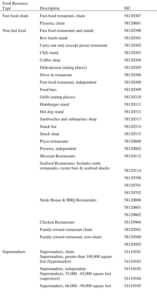
Table 2. Detailed food resource definitions based on 8-digit Standard

Industrial Classification (SIC) codes……...………..37

Table 3. Individual-level characteristics by year: the Coronary Artery Risk Development in Young Adults (CARDIA) Study,

1985-2006………39

Table 4. Neighborhood-level characteristics [median (interquartile range)] across exam year: the Coronary Artery Risk Development in

Young Adults (CARDIA) Study, 1985-2006………....40

Table 5. Neighborhood-level characteristicsa _{[median (interquartile range)]} by classesb of longitudinal neighborhood SES residents by exam year: the Coronary Artery Risk Development in Young Adults

(CARDIA) Study, 1985-2006……….……..41

Table 6. Model estimatesa of neighborhood food resourcesb predicted for classesc of neighborhood SES residents: the Coronary Artery Risk Development in Young Adults (CARDIA) Study,

1985-2006…...……….……..36

Table 7. Post-estimateda _{linear contrasts of neighborhood food} resourcesb for classesc of longitudinal neighborhood SES residents at exam years 0, 7, 10, 15, and 20: the Coronary Artery Risk Development in Young Adults (CARDIA)

Study, 1985-2006. ……….45

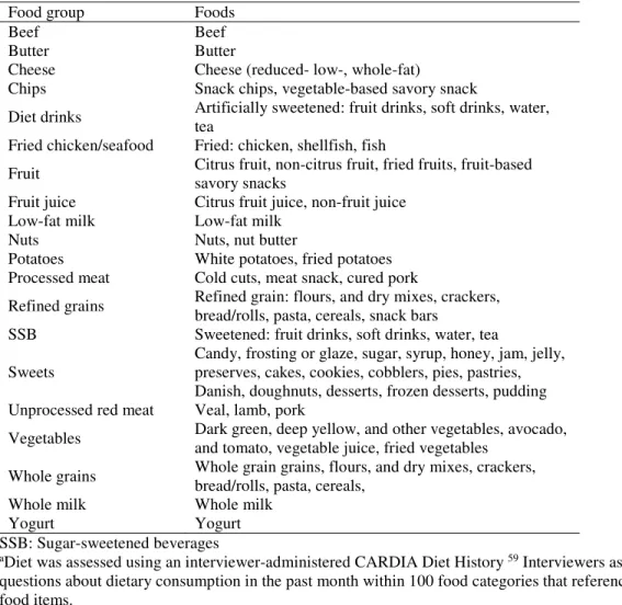
Table 8. Specific Foodsa and Beveragesa Included in Each Food Groupb _{to Model Latent factors for Hypothesized Diet}

Behaviors……….…………..70

Table 9. Reported Diet Behaviors (Range) Classified Into Low, Medium, and High Categories Across Exam Year: the Coronary Artery Risk Development in Young Adults

(CARDIA) Study, 1985-2006, n=5,114……...………..71

Table 10. Detailed Food Store and Restaurant Types Based on 8-digit Standard Industrial Classification (SIC)

Codes………...………...74

Artery Risk Development in Young Adults (CARDIA),

1985/1986 to 2005/2006, n=5,114……….80

Table 12. Neighborhood-level Characteristics Across Exam Year: the Coronary Artery Risk ]Development in Young Adults

(CARDIA) Study, 1985-2006………..………..81

Table 13. Model Fit Estimates From Structural Equation Models Examining the Pathways From Neighborhood Restaurants to BMI Through Hypothesized Diet Behaviors:the Coronary Artery Risk Development in Young Adults (CARDIA) Study,

1985-2006, n=5,114………...………82

Table 14. Standardized factor loadings from structural equation

measurement modelsa for latent neighborhood food resource and diet behavior variables: the Coronary Artery Risk

Development in Young Adults (CARDIA) Study,

1985-2006………..85

Table 15. Standardized Estimates From Structural Equation Modelsa Examining the Direct Pathways From Neighborhood Food Resources to BMI: the Coronary Artery Risk Development

in Young Adults (CARDIA) Study, 1985-2006, n=5,114. ………...………88

Table 16. Specific Foodsa and Beveragesa Included in Each Food Groupb to Model Latent factors for Hypothesized Diet

Behaviors………...………..110

Table 17. Reported Diet Behaviors (Range) Classified Into Low, Medium, and High Categories Across Exam Year: the Coronary Artery Risk Development in Young Adults

(CARDIA) Study, 1985-2006, n=5,114………...111

Table 18. Detailed Food Store and Restaurant Types Based on 8-digit

Standard Industrial Classification (SIC) Codes…...………...114

Table 19. Individual-level Characteristics by Exam year: Coronary Artery Risk Development in Young Adults (CARDIA),

1985/1986 to 2005/2006, n=5,114………...120

Table 20. Neighborhood-level Characteristics Across Exam Year: the Coronary Artery Risk Development in Young Adults

LIST OF FIGURES

Figure 1. Temporal changes in neighborhood SES characteristicsa, by 4 classesb _{of longitudinal neighborhood SES resident} characteristics: the Coronary Artery Risk Development

in Young Adults (CARDIA) Study, 1985-2006………..…..47

Figure 2. Estimated mean densitiesb of neighborhood fast food and non-fast food restaurantsb by 4 classesc of longitudinal

neighborhood SES residents characteristics: the Coronary Artery Risk Development in Young Adults (CARDIA)

Study, 1985-2006………...………..…..48

Figure 3. Estimated mean densitiesa _{of neighborhood supermarkets} and convenience storesb by 4 classesc of longitudinal neighborhood SES residents characteristics: the Coronary Artery Risk Development in Young Adults (CARDIA)

Study, 1985-2006………...………..…..49

Figure 4. Diet Behaviors Hypothesized to be Associated with

Neighborhood Food Resources.………...………..76

Figure 5. Conceptual Model of Temporal Associations Among Direct Pathways from Neighborhood food Environment to BMI, and Indirect Pathways from Neighborhood Food

Environment to BMI Through Diet……….…..77

Figure 6. Conceptual Model of Confounding Among the Direct Associations BetweenNeighborhood Food and BMI, and

Indirect Relationships Through Diet………..78

Figure 7. Conceptual Model of Indirect Pathways from Neighborhood Restaurants and Food Stores to BMI Mediated Through

Hypothesized Diet Behaviors………...…….79

Figure 8a. Standardized Estimates From Structural Equation Models Examining the Indirect Pathways From Neighborhood

Restaurants to BMI Mediated by Hypothesized Diet Behaviors: the Coronary Artery Risk Development in Young Adults

(CARDIA) Study, 1985-2006, n=5,114……….83

Figure 8b. Standardized Estimates From Structural Equation Models Examining the Indirect Pathways From Neighborhood Food Stores to BMI Mediated by Hypothesized Diet Behaviors: the Coronary Artery Risk Development in Young Adults

Figure 9a. Standardized Estimates From Sensitivity Structural Equation Models Examining the Indirect Pathways From Neighborhood Restaurants to BMI Mediated by Hypothesized Diet Behaviors, Using Fast Food Consumption at Exam Years 0, 7,10, 15, and 20: the Coronary Artery Risk Development in Young Adults

(CARDIA) Study, 1985-2006, n=5,114. ……..……….89

Figure 9b. Standardized Estimates From Sensitivity Structural Equation Models Examining the Indirect Pathways From Neighborhood Restaurants to BMI Mediated by Hypothesized Diet Behaviors, Using Fast Food Consumption at Exam Years 0, 7,10, 15, and 20: the Coronary Artery Risk Development in Young Adults

(CARDIA) Study, 1985-2006, n=5,114. ………...89

Figure 10. Diet Behaviors Hypothesized to be Associated With Neighborhood

Restaurants and Food Stores………116

Figure 11. Conceptual Model of Reverse Pathways and Temporal Relationships among Direct Pathways from Neighborhood Food Environment to BMI, and Indirect Pathways Through

Diet………...………117

Figure 12. Conceptual Model of Confounding Among the Direct Relationships Between Neighborhood Food and BMI,

and Indirect Relationships Through Diet………..…...118

Figure 13. Conceptual Model of Indirect Pathways from Neighborhood Restaurants and Food Stores to BMI Through Hypothesized Diet

Behaviors………..……...119

Figure 14a. Standardized Beta Estimates From Structural Equation Models Examining the Indirect Pathways From Neighborhood

Restaurants to BMI Mediated by Hypothesized Diet Behaviors Without Reverse Pathways: the Coronary Artery Risk

Development in Young Adults (CARDIA) Study, 1985-2006,

n=5,114………122

Models Examining the Indirect Pathways From Neighborhood Food Stores to BMI Mediated by Hypothesized Diet Behaviors Without Reverse Pathways: the Coronary Artery Risk Development

in Young Adults (CARDIA) Study, 1985-2006, n=5,114………...124

Figure 15b. Standardized Beta Estimates From Structural Equation Models Examining the Indirect Pathways From Neighborhood Food Stores to BMI Mediated by Hypothesized Diet Behaviors

With Reverse Pathways: the Coronary Artery Risk Development

LIST OF ABBREVIATIONS

BMI Body Mass Index

CARDIA Coronary Artery Risk Development in Young Adults

CFI Comparative Fit Index

FPL Federal Poverty Level

HS High school

HU Housing Unit

kg kilogram

m meter

SEM Structural equation modeling

SES Socioeconomic status

SD Standard deviation

SSB Sugar-sweetened beverage

RMSEA Root mean square error approximation

CHAPTERI:INTRODUCTION

A. BACKGROUND

Obesity increased dramatically nationwide during the mid-1980’s to 2006, with

socioeconomically disadvantaged populations disproportionately affected.1,2 _{Disparities in}

obesity have lead researchers to investigate the degree to which disadvantaged neighborhoods

have poor food environments that may promote the over-consumption of unhealthy energy-dense

foods.3-6 _{The idea that policies could reduce health disparities by modifying features of the built}

environment lead to efforts that targeted food resources.7-9 Despite the theoretical appeal of this

approach, there remains a paucity of high-quality evidence supporting these activities. The

largely cross-sectional evidence base about socioeconomic disparities in the food environment is

mixed with both positive and negative findings.10-13 Without rigorous scientific evidence it is

unlikely that any efforts to reduce obesity by modifying food environments will be effective.

Shifts in neighborhood socioeconomics that co-occur with changes in the food

environment may underlie existing equivocal evidence. In addition, most research focuses on a

single part of the pathway, generally either the associations between food resources and diet

behaviors or the association between food resources and body mass index (BMI). Yet, the extent

to which changing food environments lead to dietary change and consequent reduction in

obesity, through diet, is unknown. In addition, when estimating associations between

preferences shaping residential neighborhood selection) is often ignored and could bias relevant

pathways.

To address these limitations, we capitalized on a large and unique Geographic

Information Systems (GIS) database of neighborhood features linked to Coronary Artery Risk Development in Young Adults (CARDIA) respondent residential locations. CARDIA is a longitudinal cohort study of 5,114 black and white young adults (aged 18-30 at baseline in

1985-86). We used two decades (1985-86 to 2005-06) of time-varying data on neighborhood-level

food resources, U.S. Census data, individual-level detailed diet, anthropometric, and

sociodemographic and behavior data.

First, we used latent class analysis to identify different longitudinal patterns of

neighborhood SES indicators. The exposure to neighborhood SES over time is a latent construct

that is not measured by any single demographic variable, rather it is a combination of

neighborhood characteristics over time. By using this method we parsimoniously quantified SES

using a number of these neighborhood characteristics and captured each participants 20-year

exposure to neighborhood SES. Second, we built a structural equation model (SEM) to delineate

the complex relationships between changes in neighborhood food environment and changes in

diet and BMI. SEMs refer to modeling techniques that are equipped to handle multiequation

models, multiple measures of concepts (e.g., latent constructs), and measurement error. We

simultaneously estimated separate longitudinal pathways from neighborhood fast food

restaurants, sit-down restaurants, supermarkets, and convenience stores to BMI through diet

behaviors. While many studies examine only one type of food resource (e.g., supermarkets), our

investigated how these relationships differed by sex, race and neighborhood socioeconomics.

Third, to approximate reverse causality, we explicitly investigated reverse pathways from

predicted and time period-specific diet behaviors to future neighborhood food resources. The

prospective, longitudinal design, exceptionally varied range of social, demographic, behavioral,

and community exposure and anthropometric data allowed an outstanding opportunity to

investigate how different types of neighborhood restaurants and food stores contribute to obesity

disparities through diet across a major lifecycle period of risk for weight gain.

B. SPECIFIC AIMS

The overall goal of this research was to characterize how temporal changes in

neighborhood food resources influence diet behaviors, and through this pathway influence

weight gain in young adults followed over 20 years. Further, we examined whether these

pathways varied by socioeconomic and sociodemographic factors, and studied the potential

influence of reverse causality on our estimates from the food environment to BMI through diet

behaviors. We achieved this goal through the following aims:

1) Identify longitudinal pathways from four types of neighborhood food resources (fast

food restaurants, sit-down restaurants, supermarkets and convenience stores) to BMI

through diet behaviors and test how the pathways vary by race, sex, and longitudinal

neighborhood socioeconomic status (SES) patterns.

a. Using latent class analysis (LCA), classify individuals according to varying levels of

20-year exposure to dynamic neighborhood socioeconomic domains (e.g., occupation,

poverty, education) and determine how the availability of the four types of neighborhood

b. Develop a structural equation model to delineate the longitudinal pathways from each

type of neighborhood food resource to BMI, specifically the indirect pathways to BMI

through diet behaviors.

c. Test statistical interactions by individual-level sex, race, and the longitudinal

neighborhood SES classes derived in Aim 1a to test how neighborhood food resources

influence diet behaviors differently for males versus females, blacks versus whites, and

for CARDIA participants living in neighborhoods in declining versus improving or stable

SES.

2) Approximate reverse causality to observe how it might bias the associations observed in

the Aim 1 analyses. We will test this by extending our models in Aim 1 to include the

reverse pathways from predicted and time period-specific diet behaviors to future

CHAPTER II: LITERATURE REVIEW

A. THEIMPORTANCEOFTHEFOODENVIRONMENTANDDISPARITIESINTHE

UNITEDSTATES

Obesity rates have increased drastically in the last few decades nationwide, yet

socioeconomically disadvantaged populations are disproportionately affected.1,2 _{Unequal food}

environments are related to neighborhood socioeconomic status (SES).2,6 As such, neighborhood

food resources have been linked to disparities in obesity and poor diet.10-13 _{National and local}

efforts have targeted environmental food resources as a means to improve diet quality and

physical activity in disadvantaged areas.7-9 Yet, the obesity gap continues to widen.14 Few

longitudinal analyses have focused on diet as a proximal outcome to obesity or BMI, and these

have yielded findings that suggest complex relationships. For example, supermarket availability

bore no relation to prospective diet quality15 _{perhaps because supermarkets sell healthy and}

unhealthy foods or current statistical modeling strategies do not account for dynamic changes in

the environment or the multiple types of food resources from which individuals choose to

patronize.

Increased consumption of foods away-from-home has paralleled the obesity epidemic16

and the frequent consumption of quick-service convenience foods (e.g., burgers, fries, pizza,

sodas, etc.) characterized by poor nutrient quality, high fat, salt and added sugars predicts higher

B. NEED FOR LONGITUDINAL STUDIES

Much of the findings from cross-sectional data are mixed21-23 but in general there is

evidence, albeit from weak designs that neighborhood food resources are associated with obesity,

BMI, and some diet behaviors.10-12 _{However, cross-sectional analyses of neighborhood health}

effects lack the ability to examine bi-directional relationships and are particularly vulnerable to

selection bias. Individual personal preferences may drive neighborhood choice and may create

spurious associations between neighborhood environment and obesity related behaviors.

C. CONSIDERATION FOR MUTLIPLE TYPES OF FOOD RESOURCES

Research has focused on “food deserts”, generally defined as areas with limited access to

affordable fresh foods from supermarkets.13,23-25 Subsequently, “food swamps”,26,27 characterized

as neighborhoods with disproportionate access to convenient, energy dense, nutrient poor foods

sold by convenience stores and fast food restaurants, emerged as important dimensions of the

food environment. Thus, attention to a variety of food resources, such as supermarkets,

convenience stores, sit-down, and fast food restaurants is a more useful approach to examining

neighborhood food access than considering only one type hypothesized to sell either healthy or

unhealthy foods.13,28,29

Supermarkets and sit-down restaurants may promote a better diet because they can sell

higher quality foods than fast food restaurants and convenience stores but they also sell large

portions of processed, high fat and sugar foods. However, when we expect to see “food deserts”

in dense urban low income and high minority neighborhoods, we do also observe areas with

greater supermarket store availability than more affluent urban neighborhoods.6 _{A better}

restaurants, influence the consumption of foods that promote or protect against weight gain is

needed.

D. THEBLACKBOX

While research on the food environment, diet behaviors, and body weight has proliferated

over the past several years, most of this research ignores the multiple pathways from

environment to BMI through diet behaviors.30-32 _{Thus, the bulk of the literature involves a black}

box step from the food environment to BMI and is largely mixed (see reviews 12,33). In one of the

few longitudinal studies, Block et al. 5 found no consistent association between neighborhood

fast food and full-service restaurants with BMI in Framingham, MA adults. Yet, the Block et al.

study did not address the pathway to BMI through diet and lacking predicted diet behaviors as a

function of the food environment in their analysis may have confounded their findings.

E. NEIGHBORHOODSES,SEX,ANDRACEAREOFTENOVERLOOKED

In the few existing longitudinal analyses of neighborhood health effects on diet and BMI

there is evidence that neighborhood features, including fast food availability, are differentially associated with obesity related behaviors by sex.15,34,35 Neighborhood SES has been associated

with an increased prevalence of the metabolic syndrome among women but not men in the

Atherosclerosis Risk in Communities Study (ARIC).36 This suggests women have different diet

behaviors than men in response to features of the neighborhood that are related to SES, such as

the availability of unhealthy and healthy foods from different stores and restaurants.

In cross-sectional analyses, allocation of neighborhood food resources depending on

income has received the most focus, with some examination of differences according to race. For

example, the influence of the neighborhood food environment on fruit and vegetable intake

characteristics have been associated with modest increases in CVD mortality in white

participants, this was not the case for African American participants in ARIC.38 Similarly,

inconsistent associations with neighborhood advantage were documented for serum cholesterol

and disease prevalence in African-American men.39 _{Carson et al. also observed a significant}

association between neighborhood SES and mean intima-media thickness among whites, but not

blacks.40 _{Evidence of substantial heterogeneity in black-white hypertension differences}

depending on geographic group was observed in MESA.41 Lastly, among CARDIA participants,

insulin resistance was inversely associated with increasing neighborhood SES in white men and

women but this association was only observed among black participants who had high income

and education.42 Different relationships between the environment and cardiometabolic outcomes

for white and African Americans may reflect race specific diet behaviors in response to

neighborhood disadvantage and poor food availability that lead to increased BMI and adverse

cardiometabolic consequences.

Consideration of neighborhood socioeconomic status in relation to disparities in the food

environment yielded inconsistent results even in national samples.29,43-45 This suggests that there

may be unmeasured complex relationships between neighborhood SES and features of the food

environment. Complex relationships between neighborhood SES and the food environment are

difficult to capture. Neighborhood SES cannot be explicitly measured. Instead it is a latent

construct comprised of multiple SES domains such as income and wealth, education, occupation,

and housing. Multiple aspects of neighborhood SES may track together over time, such as

poverty and unemployment. However, there may also be other aspects of neighborhood SES that

housing because the property taxes are lower than in a low income neighborhood with no vacant

housing. 46 Our proposed longitudinal neighborhood SES classes captured the neighborhood

sociodemographics race, poverty, education, unemployment, income, and real estate value that

change across exam years.

F. REVERSECAUSALITY

Neighborhoods, comprised by social, natural, and built environments, can be defined

broadly as something that surrounds and influences populations and is a dynamic component of

population health. Relationships between the individuals and the environment are bi-directional;

people choose their surroundings and conversely, the environment affects people such that

everyday lifestyle choices that impact health are made in the context and constraints of the

environment. Evidence suggests the preference for neighborhood amenities guides residential

location choice and can have a direct association with behavior. 47-52 In a cross-sectional survey,

participants reporting access to public transit as a priority for residential location were almost 20

times more likely to use rail transit than those who did not cite this preference. 53 _Furthermore,

recent surveys suggest increasing preferences for traditionally designed communities (e.g.,

centrally located retail, alternative transportation infrastructure) among a nationally

representative sample of US adults.54 In addition there is evidence that desiring to live in an

activity-friendly community is predicted by beliefs that an activity friendly community will

support active transit.55 _{There is substantial evidence that race and income are important factors}

in residential mobility, migration, and housing choice.56-58 Residential location choice is complex

and driven by more than dietary preferences. However, individual diet preferences and behaviors

may be tied to unobserved characteristics _{(e.g., culture, health consciousness, and social ties)}

to environment) will bias any paths we estimate in the other direction (environment to

individual). Structural equation modeling (SEM) can model these simultaneous or bi-directional

paths.

G. METHODSARELACKING

Longitudinal methods that employ fixed effects models may provide insight into

residential selection bias because they obviate confounding by unmeasured time invariant

aspects. But fixed effect models cannot address the confounding due to unmeasured time varying

characteristics. Furthermore, estimation of direct effects from the broad environment to

individual obesity or BMI will miss the necessary path through diet. The food resources in a

neighborhood can only influence BMI through an effect on individual diet. SEM can account for

the bi-directional relationship between diet and the food environment and estimate effects of

latent (unmeasured) characteristics that vary over time.

H. SUMMARY

There are few longitudinal studies of the food environment, diet, and BMI and there are

even fewer that use sophisticated modeling to address complex pathways from the environment

to BMI through diet. The prospective, longitudinal design, exceptionally varied range of data

allow an outstanding opportunity to characterize how different types of neighborhood restaurants

and food stores contribute to obesity disparities through diet across a major lifecycle period of

risk for weight gain. In sum, through the proposed analyses we characterized how temporal

changes in neighborhood food resources influence diet behaviors, and through this pathway

influenced weight gain in young adults followed over 20 years. Further, we examined whether

and come one step closer towards understanding how individual effects on the food environment

bias associations from the food environment to the individual.Our findings will inform policies

CHAPTER III:METHODS

A. STUDYPOPULATIONANDDATASOURCES

The Coronary Artery Risk Development in Young Adults (CARDIA) study is a longitudinal cohort with detailed diet, clinic, physical activity, environmental, and

sociodemographic data collected for 5,114 white or black United States (U.S.) adults aged 18-30

years. Throughout 20 years of follow-up data derived from a geographic information system

(GIS) was linked temporally and geographically to respondents residential locations at the time

of each exam.

CARDIA

Respondents were recruited originally from 4 centers: Birmingham, AL; Chicago, IL;

Minneapolis, MN; and Oakland, CA. Participants were selected in 1985-86 with approximately

equal numbers by race, gender, education (high school or less versus more than high school), age

(18-24 years versus 25-30 years) within each center, and followed over 25 years. The GIS is

currently linked to exam years 0, 7, 10, 15, and 20. However, linking the GIS to year 25 data is

BODY MASS INDEX

At each examination, participants’ weight was measured to the nearest 0.2 kg and height

was measured to the nearest 0.5 centimeter. BMI is calculated as weight in kilograms divided by

height in meters squared and measured at exam years 0, 7, 10, 15, and 20.

DIETARY ASSESSMENT

An interviewer-administered CARDIA Diet History 59 _{at exam years 0, 7, and 20 was}

used to assess diet. Interviewers asked open-ended questions about dietary consumption in the

past month within 100 food categories that referenced 1609 separate food items. Nutrients and

food groups were assigned by the University of Minnesota Nutrition Coordinating Center

(NCC). We further combined NCC-assigned food groups into one of 13 food groups and 5

beverage groups [assessed as servings per day of constituent foods (Web Table 1)] shown to be

associated with weight change per 4-year period in the Nurse’s Health Study I and II, and the

Health Professionals Follow-up Study 19 and cardiometabolic outcomes.60 We also used survey

data collected at exam years 0, 7, 10, 15, and 20 regarding the number of times per week

respondents ate meals at fast food restaurants.18 We categorized weekly fast food consumption

and servings per day of consumed foods and into low, medium, or high consumption, either by

year-specific tertiles or as non-consumers (0 servings per day) versus upper and lower

distributions of consumers (≥1 serving per day), values defined in Web Table 2. We used

year-specific tertiles to allow for temporal changes in diet behaviors.

We set reported diet behaviors and BMI to missing when participants had extreme energy

intakes 61 _{[<800 or >8000 kcal/d for men (n=73 at year 0, n=60 at year 7, and n=25 at year 20);}

and <600 or >6000 kcal/d for women (n=53 at year 0, n=34 at year 7, and n=29 at year 20)] or

GIS DATABASE

Our Obesity and Environment database is a unique and large GIS that links biologic, and

behavior data to environment indicators over time. It provides tremendous opportunities to study

multi-level determinants of obesity and inform policies with the goal to address inequalities in

disadvantaged communities and reduce obesity disparities in vulnerable populations. It contains

many community-level variables including counts of many types of food resources, roadway

length, population density and sociodemographics that are linked temporally and spatially to

CARDIA each participant’s individual-level clinic, behavior, and anthropometric data.

B. ANALYTIC VARIABLES

NEIGHBORHOOD FOOD ENVIRONMENT

We obtained counts of chain fast-food restaurants (hereafter referred to as fast food

restaurants), all other restaurants not classified as chain fast food (hereafter referred to as

sit-down restaurants), supermarkets, and convenience stores from Dun and Bradstreet (D&B), a

commercial dataset of U.S. business records using 8-digit Standard Industrial Classification

(SIC) codes for years 7, 10, 15, and 20 and a combination of 4 digit SIC codes and matched

business names at year 0 (Web Table 3). D&B includes many other food resources however, we

focused on the types that were conceptually more stable drivers of diet behaviors, We used a

3-km Euclidean buffer around each respondent’s residential location for restaurants 15,62 _{and an}

8-km Euclidean buffer for food stores, 62,63 based on empirical evidence. Using StreetMap 2000

www.esri.com: Redlands, CA), we calculated densities of restaurants and stores as counts per 10

km secondary roads (to connect smaller towns, subdivisions, and neighborhoods) and local roads

(for local traffic, usually with a single lane of traffic in each direction), resulting in a measure of

concentration of food resources along streets representing overall commercial activity.64,65 _We

also included variables reflecting urbanicity and development as these relate directly to the food

environment. Given that population density varies across roadway structure 66 _{and across rural}

versus urban areas;67 population density and commercial development were independently

associated with geographic food resource distribution and were not highly correlated in our data

ρ=0.35. Therefore, we included population density (representing area-level development and

population) and counts per roadway (representing commercial development) in our analyses.

AREA-LEVEL SOCIOECONOMIC INDICATORS

Neighborhood SES was derived at the U.S. census tract-level at all years; tract-level SES

is more strongly associated with health outcomes as compared to block group-level SES.68,69

Neighborhood SES is a latent construct comprising multiple SES domains and is an

individual-level exposure; that is, people may experience temporal changes in neighborhood SES through

residential movement or changes in their neighborhood. In addition, food environments may

improve or worsen over time, and these dynamics may relate to neighborhood SES. We included

multiple measures of socioeconomic disadvantage that reflect the domains of income, education,

race, employment, and housing value from years 0, 7, 10, 15, and 20: % race white, % education

<high school, % poverty (below 150% federal poverty level70), % unemployed, %

professional/management occupation, median income, % vacant housing, aggregate housing

value, % owner occupied, and median rent. We also used population density (census tract

INDIVIDUAL-LEVEL CONFOUNDERS

We characterized individual-level confounders using data from structured interview or

self-administered questionnaire collected at each exam year. Time-invariant sociodemographic

variables were sex, race (white/black), exam attendance, and center. Time-varying characteristics

were maximum reported number of years of schooling completed by the exam year (continuous),

and mean household income inflated to U.S. dollars at year 20 (2005-06) using the Consumer

Price Index. Income was not collected in year 0, so we used the closest measurement (year 5) for

CHAPTER IV: NEIGHBORHOOD SOCIOECONOMIC STATUS AND FOOD ENVIRONMENT: A 20-YEAR LONGITUDINAL LATENT CLASS ANALYSIS AMONG

CARDIA PARTICIPANTS1

A. ABSTRACT

Cross-sectional studies suggest neighborhood socioeconomic (SES) disadvantage is associated

with obesogenic food environments. Yet, it is unknown how exposure to neighborhood SES

patterning through adulthood corresponds to food environments that also change over time. We

used latent class analysis (LCA) to classify participants in the U.S.-based Coronary Artery Risk

Development in Young Adults study [n=5,114 at baseline 1985-1986 to 2005-2006] according

to their longitudinal neighborhood SES residency patterns (upward, downward, stable high and

stable low). For most classes of residents, the availability of fast food and non-fast food

restaurants and supermarkets and convenience stores increased (p<0.001). Yet,

socioeconomically disadvantaged neighborhood residents had fewer fast food and non-fast food

restaurants, more convenience stores, and the same number of supermarkets in their

neighborhoods than the advantaged residents. In addition to targeting the pervasive fast food

restaurant and convenient store retail growth, improving neighborhood restaurant options for

disadvantaged residents may reduce food environment disparities.

B. INTRODUCTION

From the mid-1980’s to the 2000’s, obesity increased dramatically in developed

countries, such as the U.S., U.K., New Zealand, and Canada72 with socioeconomically

disadvantaged populations disproportionately affected.73,74 _{Disparities in obesity have lead}

researchers to investigate the degree to which disadvantaged neighborhoods have poor food

environments that promote the over-consumption of unhealthy foods.3-6 Identifying modifiable

features of the food environment hypothesized to influence individual-level diet behaviors could

lead to effective policies that will improve health in disadvantaged populations. However, the

largely cross-sectional evidence base about socioeconomic disparities in the food environment is

mixed with positive and negative findings.10-13 _{Complexities resulting from temporal patterns in}

neighborhood modifications and residential mobility may underlie existing equivocal evidence.

Several large international obesity literature reviews recognize the need for

comprehensive strategies and systems models75,76 and attention to wider environmental and

societal factors in efforts to reduce obesity disparities. Nonetheless, socioeconomically

disadvantaged subpopulations in developed countries remain disproportionately affected by

obesity.77 Thus, there is growing interest by researchers in the U.S. and other developed

countries on the role of socioeconomic factors in temporal declines in healthy food

environments.78-81 But findings are mixed and studies examining temporal patterns in food

environments are sparse (see review33_{). There is a large gap in long-term, population-based}

In particular, two major gaps in the literature limit our understanding of inequities in the

food environment. First, how does exposure to socioeconomic aspect of neighborhoods change

through the life course? Second, do patterns of change in the neighborhood SES environment

also reflect changes in exposure to different types of food resources? Understanding the

relationships between these two aspects of longitudinal neighborhood exposures may shed

insight on how to effectively modify food environments for socioeconomically disadvantaged

populations to improve diet and reduce obesity.

Complex relationships between neighborhood SES and the food environment are difficult

to capture. Neighborhood SES cannot be explicitly measured. Instead it is a latent construct

comprised of multiple SES domains such as income and wealth, education, occupation, and

housing. Multiple aspects of neighborhood SES may track together over time, such as poverty

and unemployment. However, there may also be other aspects of neighborhood SES that drive

commercial zoning policies or economic incentives for food retailers. For instance, supermarket

owners may be more likely to locate in a low income neighborhood with vacant housing because

the property taxes are lower than in a low income neighborhood with no vacant housing.46

Another layer of complexity underlying relationships between neighborhood SES and the

food environment is that, as individuals experience neighborhood SES changes over time,

heterogeneities and similarities may develop within and across socioeconomic domains. For

example, at the community-level vacant housing and the number of residents living in poverty

may increase steadily in one neighborhood over time, while in another neighborhood, residents

may attain higher levels of education but community-level household income may not increase

until after graduates have entered the workforce. As an individual-level exposure, people may

neighborhoods. In addition, depending on neighborhood SES, food environments may improve

or worsen over time. Therefore, a single snapshot in time may not capture patterns of

socioeconomic characteristics that drive greater or reduced access to different types of food

stores and restaurants.

To overcome these gaps in the literature, we capitalized on a geographic information system (GIS)-derived dataset in the United States (U.S.) spatially and temporally linked to Coronary Artery Risk Development in Young Adults (CARDIA) respondent residential locations

at each of five exam years occurring over a 20-year period. We examined how individuals were

exposed to different patterns of multiple neighborhood SES characteristics (e.g., occupation,

poverty, and education) during young to middle adulthood using Latent Class Analysis (LCA).

The result was a classification of CARDIA participants according to 20 years of their

time-varying neighborhood SES characteristics. During a period when adult obesity increased rapidly

in the U.S. we examined how neighborhood fast food restaurants, non-fast food restaurants,

supermarkets, and convenience stores compared over time for adults across longitudinal

neighborhood SES patterns. We hypothesized that participants with a 20-year history of living in

socioeconomically disadvantaged neighborhoods were exposed to worse food environments (i.e.,

few supermarkets and more fast food restaurants) that deteriorated over time compared to those

with a history of living in advantaged neighborhoods.

C. METHODS

years originally from 4 centers: Birmingham, AL; Chicago, IL; Minneapolis, MN; and Oakland,

CA. Participants were selected in 1985-86 with approximately equal numbers by race, gender,

education (high school or less versus more than high school), age (18-24 years versus 25-30

years) within each center, and followed over 5 exams during 1992-93 (Year 7), 1995-96 (Year

10), 2000-01 (Year 15), and 2005-06 (Year 20). Retention rates were 81%, 79% , 74% , and

72% , respectively, of the surviving cohort.

We used data from 5 exam years (0, 7, 10, 15, and 20) and a GIS-derived dataset of time-varying neighborhood-level food resources and U.S. Census data were spatially and temporally linked to CARDIA respondent residential locations at each exam year.

AREA-LEVEL INDICATORS

U.S. Census block groups were not available in the 1980 census data (year 0) so census

tracts were used to define neighborhoods at all years. Census tract measures have been shown to

identify health disparities as well as, if not better than, block groups.68,69 The geographic area of

U.S. Census tracts depends on population density, with an optimum size tract of 4,000 people,

although census tracts range from 1,200 to 8,000 people.82 At baseline, the catchment area of the

four CARDIA centers comprised 799 Census tracts, by 2005-06 as individuals moved out of the

original four field site cities, the catchment increased to include 2,800 tracts. We included

multiple measures of socioeconomic disadvantage that addressed the domains of income,

education, race, employment, and housing value (Table 1). Population density was calculated as

tract population per square kilometer of land excluding water; it was not included in the LCA but

was included as a covariate in multivariable models to adjust for area-level development.

other restaurants not classified as chain fast food (hereafter referred to as non-fast food

restaurants), supermarkets, and convenience stores were obtained from Dun and Bradstreet

(D&B), a commercial dataset of U.S. business records. They were classified according to 8-digit

Standard Industrial Classification (SIC) codes (Table 2) for years 7, 10, 15, and 20. Year 0 SIC

codes were 4 digits; this limited the specificity of restaurant classification, so fast food

restaurants were identified by matching business names with fast food restaurants at years

1991-1996 and by SIC code. Fast food restaurants, non-fast food restaurants, supermarket, and

convenience stores were aggregated as counts within 3 kilometers (km) of each respondent’s

residential location (Euclidean buffer). The 3 km buffer was chosen to capture distances readily

accessible by walking and driving to neighborhood diet-related resources as supported by several

studies.62,64,83 _{Food resource densities were derived as counts per 10 km secondary roadway}

(roads used to connect smaller towns, subdivisions, and neighborhoods) and local roadway

(roads used for local traffic, usually with a single lane of traffic in each direction), resulting in a

measure of concentration of food resources along streets representing overall commercial

activity.64,65 Roadway lengths were calculated from street networks extracted from StreetMap

2000 (v. 9.0) for years 7 (1993) and 10 (1996), from StreetMap Pro 2005 (v. 5.2) for year 15

(2001), and from StreetMap Pro 2010 (v. 7.2) for year 20. Street network source datasets were

obtained from Environmental Systems Research Institute (ESRI, www.esri.com: Redlands, CA).

We opted for the roadway-scaled measures rather than raw food resource counts because count

measures can introduce spurious associations between neighborhood SES and food stores and

restaurants. For example, low SES neighborhoods may have more convenience stores because

and thus might obscure disparities in the food environment by neighborhood SES. While we did

not use network buffers, we addressed differences in food resources according to overall

commercial activity by scaling counts by roadway length while holding Euclidean area constant

across geographic areas varying in terrain and network distances. Thus, the resources relative to

roadway lengths provides measures relative to road network, whereas the Euclidean buffers

provide the salient geographic area of focus.

INDIVIDUAL-LEVEL CHARACTERISTICS

Individual-level sociodemographics were used to describe the study population

throughout the study period. Sociodemographics were collected at each exam year by a

structured interview or self-administered questionnaire. Sex, race (white/black), exam

attendance, and center were time-invariant variables. Time-varying individual-level

characteristics included working full-time (yes, no), marital status (married, not married),

maximum reported number of years of schooling completed by the exam year (less than high

school, high school, some college, college degree or above), and mean household income

inflated to U.S. dollars at year 20 (2005-06) using the Consumer Price Index. Income was not

collected in year 0, so the closest measurement (year 5) was used for year 0.

STATISTICAL ANALYSES

All descriptive analyses and multivariable models were performed using Stata 13.0

(StataCorp, College Station, TX).

Descriptive statistics. To describe the study population and their neighborhoods over exam years

0, 7, 10, 15, and 20, we calculated means and standard deviations (continuous variables) and

Latent class analysis: derivation of longitudinal neighborhood SES classes. We performed LCA

models with Mplus84 to classify CARDIA respondents into longitudinal neighborhood SES latent

classes according to Census demographics. All variables used in the LCA were transformed to

year-specific standard normal deviates [(X- mean)/SD] (hereafter referred to as Z-scores) to

facilitate convergence of the LCA models. The variables related to housing were transformed to

Z-scores specific to CARDIA study center, to account for the large cost of living differences

between centers. Residential mobility was not included in these analyses because our aim was to

quantify exposure to patterns of neighborhood SES over time, regardless of mobility.

A two-class model was estimated first with maximum likelihood methods and then

models were considered with additional classes. We used the following criteria determine the

number of k latent classes for our final model: 1) the Bayesian Information Criteria (BIC) (model

fit and parsimony across models whereby smaller values indicate better fit); 2) the

interpretability of model solution with assessment of size and uniqueness of each class; and 3)

Lo-Mendell-Rubin (LMR) p-value (k vs. k – 1 class). A significant LMR p-value indicates that

the k-class solution is significantly different from the (k-1)-class solution, suggesting that k-class

solution is preferred. Using these criteria, interpretability, and verifying model fit with BIC, we

selected 4 SES classes.

Each individual was assigned to the single longitudinal neighborhood SES class for

whom they had the highest posterior class membership probability. A minimum number of

up visits was not an inclusion criterion and on average respondents attended most

follow-up visits (mean=3.98, SD=1.39). Class results are illustrated by plotting the mean Z-score for the

Relationship between longitudinal neighborhood SES classes with food environment measures.

Next, we compared changes in neighborhood food resources over time experienced by

participants across the four longitudinal neighborhood SES classes. Longitudinal multilevel

random effects regression models estimated each neighborhood food resource density relative to

roadway length separately as a function of SES class indicators (referent was class with largest

sample size), exam year (continuous), interaction of class indicators by exam year, and a random

effect for each participant. Population density [which can vary across roadway structure,66 rural

and urban areas67 and commercial development were each independently associated with

geographic food resource distribution and were not highly correlated in our data ρ=0.35.

Therefore, we addressed population density (representing area-level development and

population) and counts per roadway (representing commercial development) in our modeling.

Time trends were statistically significant if the p-value of the estimated marginal year effect

within class was less than 0.05. Linear contrasts (Stata’s ‘lincom’ command) compared food

resource densities relative to roadway length by year and for each class pair and marginal

predictions estimated mean food resource densities relative to roadway length by class and year.

Food environment model results are presented as: 1) plots of the estimated mean densities

relative to roadway length for each type of neighborhood restaurant and food store by class and

year; 2) table of beta coefficients from the multivariable random effects models for each food

resource; and 3) table of the linear contrasts by year and for each class pair.

D. RESULTS

Descriptive statistics. Across 20 years of CARDIA exams, participant educational attainment,

income, and proportion married increased over time (Table 3). Overall, the neighborhoods in

environment indicators (Table 4). Counts of neighborhood fast food restaurants and convenience

stores increased, non-fast food restaurants decreased, and supermarkets remained fairly stable.

Latent class analysis. CARDIA participants were classified into four latent classes of

longitudinal neighborhood SES based on BIC =610725 and LMR (p=0.04 for four vs. three

classes compared to p=0.72 for five vs four classes classes): downwardly mobile neighborhood

SES residents (n=1,014); stable low neighborhood SES residents (n=1,581); upwardly mobile

neighborhood SES residents (n=665); and stable high neighborhood SES residents (n=1,854)

(Figure 1). The average posterior probability within each class was > 0.97. In general, the LCA

components that indicated neighborhood advantage (e.g., income, aggregate housing value)

tracked together over time, as did the indicators of disadvantage (e.g., unemployment, vacancy).

Medians and interquartile ranges of neighborhood SES and food resource measures are presented

by longitudinal neighborhood SES class in Table 5.

Relationship between longitudinal neighborhood SES classes with food environment. The

plotted mean food resource densities relative to roadway length and time trends are presented by

class and year for restaurants (Figure 2) and food stores (Figure 3). In general, time trends in

each type of food resource were similar for all residents regardless of their neighborhood SES

class. Neighborhood densities of fast food restaurants, supermarkets, and convenience stores

relative to roadway length increased over time for all classes of neighborhood SES residents.

Neighborhood non-fast food restaurant density relative to roadway length increased over time for

Beta coefficients from the multivariable random effects models for each food resource

are presented in Table 6. Linear contrasts for each class pair are presented by year and food

resource in Table 7. In contrast to the time trends, fast food and non-fast food restaurant

densities relative to roadway length varied markedly across classes of neighborhood SES

residents, and the differences were stable over time. The participants belonging to the upwardly

mobile and stable high neighborhood SES residential classes had more non-fast food restaurants

in their neighborhoods at all observed years than those in the downwardly mobile or stable low

SES neighborhood classes. Likewise, stable high neighborhood SES residents and upwardly

mobile neighborhood SES residents consistently had more fast food restaurants in their

neighborhoods than downwardly mobile and stable low SES neighborhood residents. In sum,

advantaged neighborhood (stable high SES or upwardly mobile) residents consistently had more

of both types of restaurants than the disadvantaged neighborhood (stable low SES or

downwardly mobile) residents.

At most years, all residents had similar supermarket density relative to roadway length in

their neighborhoods, regardless of their neighborhood SES resident class (Table 7). While

neighborhood convenience store densities relative to roadway length were relatively similar for

all residents in the mid-1980’s over time, the downwardly mobile neighborhood SES residents

had more convenience stores in their neighborhoods than all other classes of residents.

E. DISCUSSION

Using a unique set of data covering 20 years of residential histories and latent class

analysis methods, we found that neighborhood restaurant and food store availability increased

for all residents. Further, the more advantaged neighborhood SES residents had greater

Our approach addressed two gaps in the literature: 1) How does exposure to socioeconomic

aspects of neighborhoods change through the life course? Indeed, we successfully classified

CARDIA participants into four distinct patterns of longitudinal neighborhood SES: downwardly

mobile neighborhood SES residents, stable low neighborhood SES residents, upwardly mobile

neighborhood SES residents, or stable high neighborhood SES residents. 2) Are patterns of

change in the neighborhood SES environment also associated with changes in exposure to

different types of food resources? We found that blacks and whites who lived in neighborhoods

of low or declining SES during young to middle adulthood, had consistently more convenience

stores and fewer restaurant options over time than individuals living in socioeconomically

advantaged neighborhoods.

During a period when obesity prevalence increased significantly in the U.S.,1,85

neighborhood fast food restaurant, non-fast food restaurant, convenience store and supermarket

availability also increased for most CARDIA participants. Such trends are consistent with

national reports86-89 _{and reflect macroeconomic shifts in the retail food industry.}

Two decades of residential histories in our large sample reveal disparities in how such

national trends in food retail were experienced for subpopulations with different longitudinal

neighborhood SES patterns. At any given time, those consistently living in socioeconomically

disadvantaged neighborhoods had lower neighborhood density of non-fast food restaurants

relative to roadway length than those consistently living in socioeconomically advantaged

neighborhoods. Socioeconomically advantaged neighborhood residents had more fast food and

non-fast food restaurants in their neighborhoods; therefore, they had a greater variety of

However, non-fast food restaurants, as defined here, are a heterogeneous group of restaurants

and do not necessarily represent restaurants that only sell healthy options.

Residential mobility could have resulted in more dramatic changes in food environment

exposures for individuals who moved versus those who remained in the same residential location

over the follow-up, if changes in food environment were greater among those who moved

residences. In our data, only 378 (7%) participants stayed in the same residential location

throughout the study period and the changes in neighborhood SES were actually larger in

non-movers versus non-movers (P<0.001). Among the 378 non-non-movers, 50% were classified into one of

the upwardly (7%) or downwardly (43%) mobile SES residency classes, compared to only 31%

of the movers (13% upward; 18% downward). Changes in the food environment were similar for

movers and non-movers, except that non-movers had greater temporal increases in numbers of

non-fast food restaurants and convenience stores (P<0.001). Given that residential mobility did

not predict greater changes in neighborhood SES or food environment it is unlikely that

residential mobility biased our findings.

Our findings contradict prior research showing that low income and high minority

population neighborhoods have more fast food and fewer full-service restaurants than

socioeconomically advantaged neighborhoods.90-92 However, our results concur with a large

national study that found that predominantly black neighborhoods had fewer full-service and fast

food restaurants than predominantly white neighborhoods.93

In our study, supermarket availability was similar for socioeconomically disadvantaged

compared to advantaged neighborhood residents throughout most of two decades. At the same

time, the most socioeconomically disadvantaged neighborhood residents had more convenient

with the prevailing view that neighborhood disadvantage has been associated with reduced

access to supermarkets/grocery stores. However, associations have varied by neighborhood racial

composition.6,90,94,95

In addition to the cross-sectional design, most of the above studies were geographically

limited or did not control for area-level development. Socioeconomically deprived

neighborhoods in dense urban areas may have many fast food restaurants as a consequence of

commercial development; thus, not accounting for such area-level development can create

spurious associations between neighborhood disadvantage and disparities the food environment.

In this study, respondents lived in mainly urban areas however, population density can vary

across urban areas.67 Population density and commercial development are correlated and

independently associated with dietary behaviors.96 _{We addressed commercial density by scaling}

food resource measures by roadway length and controlling for population density in regression

models.

Our findings suggest that overall fast food industry growth may have a greater impact on

diet behaviors among persons living in the most disadvantaged neighborhoods because they have

less access to alternative away-from-home eating options. Greater total food outlet density has

been inversely associated with BMI, perhaps because greater density typically offers a wider

array of food options or lower prices so that residents can make healthier food purchases97

despite rising fast food availability.86 _{Conversely, lower BMI in areas with high food outlet}

density may reflect overall dietary preferences of the residents.98 Alternatively, lower BMI and

high food outlet density may both be consequences of living in a more privileged environment,