Stochastic Weighted Graphs: Flexible Model
Specification and Simulation
*
James D. Wilson, Matthew J. Denny, Shankar Bhamidi,
Skyler Cranmer, and Bruce Desmarais
†November 10, 2016
Abstract
In most domains of network analysis researchers consider networks that arise in nature with weighted edges. Such networks are routinely dichotomized in the interest of using available methods for statistical inference with networks. The generalized exponential random graph model (GERGM) is a recently proposed method used to simulate and model the edges of a weighted graph. The GERGM specifies a joint distribution for an exponential family of graphs with continuous-valued edge weights. However, current estimation algorithms for the GERGM only allow inference on a restricted family of model specifications. To address this issue, we develop a Metropolis–Hastings method that can be used to estimate any GERGM specification, thereby significantly extending the family of weighted graphs that can be modeled with the GERGM. We show that new flexible model specifications are capable of avoiding likelihood degeneracy and efficiently capturing network structure in applications where such models were not previously available. We demonstrate the utility of this new class of GERGMs through application to two real network data sets, and we further assess the effectiveness of our proposed methodology by simulating non-degenerate model specifications from the well-studied two-stars model. A working R version of the GERGM code is available in the supplement and will be incorporated in thegergmCRAN package.
Keywords:Exponential Random Graph, Generalized Exponential Random Graph, Markov Chain Monte Carlo, Metropolis–Hastings
*The authors gratefully acknowledge the National Science Foundation and NSF grants DMS-1105581,
DMS-1310002, SES-1357622, SES-1357606, SES-1461493, and CISE-1320219.
†James D. Wilson is an Assistant Professor in the Department of Mathematics and Statistics at the
Uni-versity of San Francisco ([email protected]). Matthew Denny is a Ph.D. Candidate in the Department of Political Science and Social Data Analytics at Pennsylvania State University ([email protected]). Shankar Bhamidi is an Assistant Professor in the Department of Statistics and Operations Research at the University of North Carolina ([email protected]). Skyler Cranmer is the Carter Phillips and Sue Henry Associate Professor in the Department of Political Science at the Ohio State University ([email protected]). Bruce Desmarais is an Associate Professor in the Department of Political Science at Pennsylvania State University ([email protected]).
1
Introduction
Throughout the sciences, but particularly in the social sciences, a fundamental tool for the
statistical analysis of networks has been the exponential random graph model (ERGM) - a
popular, powerful, and flexible tool for statistical inference with network data (Holland and
Leinhardt,1981;Wasserman and Pattison,1996;Snijders et al.,2006). Despite their
pop-ularity, conventionally used ERGMs have the major limitation that they require the edges
of an observed network be binary (representing the presence or absence of an edge). Thus
ERGMs cannot directly model weighted networks. Since many substantively important
net-works are weighted, this restriction is especially problematic. Weighted netnet-works arise, for
example, in the study of financial exchange (Iori et al.,2008), migration patterns (Chun,
2008), and in the analysis of brain functionality and connectivity (Simpson et al.,2011).
Recently, some progress on modeling weighted networks in the ERGM framework was
made inDesmarais and Cranmer(2012), where the generalized exponential random graph
model (GERGM) was proposed to study networks with continuous-valued edges. Around
the same time,Krivitsky(2012) proposed the weighted exponential random graph model
that generalized the ERGM to networks with integer-valued edges.Robins et al.(1999)
de-veloped logistic dyad-independent models for networks with integer-valued edges. Though
each of these models provide a means to analyze weighted networks, we will focus on
extensions to the GERGM.
In general, the likelihood function of an ERGM is intractable (though some recent
progress has been made in the large networkn Ñ 8limit (Chatterjee et al.,2013;Lubetzky
and Zhao,2014)); however, efficient estimation can be achieved through the use of Markov
Chain Monte Carlo (MCMC) algorithms (Geyer and Thompson,1992; Hunter and
Hand-cock,2006). MCMC can be used to simulate samples of networks from which the likelihood
function of an ERGM can be approximated. Like the ERGM, estimation of the GERGM is
readily achieved via MCMC algorithms.Desmarais and Cranmer(2012) proposed a Gibbs
sampling technique for GERGM estimation; however, this strategy limits the specification of
network dependencies captured by the GERGM to those for which full conditional edge
dis-tributions can be derived in closed form. Another important obstacle that arises in discrete
which only a few network configurations usually very sparse and very dense networks
-have high probability mass (Handcock et al.,2003; Rinaldo et al.,2009;Schweinberger,
2011). The issue of degeneracy strongly influences the effectiveness of an MCMC algorithm.
Indeed, in the case that nearly empty (or nearly complete) networks are most probable,
estimation via MCMC will fail to converge to consistent parameter estimates.
Here, we expand the family of weighted networks that can be analyzed under the
GERGM by developing a Metropolis–Hastings sampling procedure that allows the flexible
specification of network statistics and models under the GERGM framework. Perhaps the
greatest drawback of the limited set of models for which Gibbs Sampling can be used to
simulate networks is that they are prone to degeneracy. This is due to the fact that the
closed-form derivation of the conditional distribution of an edge requires that the network
statistics used to specify the GERGM depend linearly on the value of each edge. GERGM
specifications that include nonlinear statistics are often required to avoid degeneracy. A
significant advantage of our proposed Metropolis–Hastings (MH) procedure is that one
can use MH sampling to estimate models that involve nonlinear network statistics. The
expanded set of GERGM specifications made available with the use of MH can be used
to find a non-degenerate model specification. Furthermore, in models where the Gibbs
sampler can be used, Metropolis–Hastings yields the same parameter estimates as those
obtained via Gibbs. The framework established here provides an important step in flexibly
modeling and simulating weighted networks while further providing a means of avoiding
model degeneracy.
In Section2, we describe the generalized exponential random graph model for graphs
with continuous-valued edges. In Section 3, we discuss the Monte Carlo maximum
like-lihood estimation of the GERGM and briefly describe the Gibbs procedure devised in
Desmarais and Cranmer(2012). At the end of Section3, we formulate a flexible Metropolis–
Hastings sampling procedure. We propose a class of model specifications in Section4that
expands the family of GERGMs beyond those permissible under Gibbs sampling. In Section
5, we evaluate the performance and potential utility of our proposed framework through
application to the U.S. state-to-state migration network, an international financial exchange
network, as well as through a simulation study that revisits the degenerate two-star-model
work in Section 6.
2
The Generalized Exponential Random Graph Model
Consider a directed network defined on a node set rns “ t1,2, . . . , nu, where m “ npn´
1q denotes the total number of directed edges between these nodes. Suppose that the weighted relationships between the nodes are represented by a collection of weights pyij :
i ‰ j P rnsq P Rm. The aim of this section is to describe a specific class of probability models on Rm as constructed in Desmarais and Cranmer (2012) called GERGMs that incorporates relational structure between the nodes to generate a random vectorY PRm. This probability distribution is specified by a joint probability density function (pdf)fYpy,Θq driven by real-valued parametersΘ.
A GERGM for the observed configurationyhas a simple generative process that relies on
two distinct steps. First, a joint distribution that captures the structure and interdependence
of Y is defined on a restricted network configuration,X P r0,1sm. Next, the restricted network X is transformed onto the support of Y through an appropriate transformation
function. These two steps are closely related to the widely studied specification of joint
distributions via copula functions (Genest and MacKay, 1986). We now describe the two
steps in specifying a GERGM in more detail.
In the first specification step, a function of network summary statistics hhh:r0,1sm ÑRp is formulated to represent the joint features ofX. The random vectorX is modeled by an
exponential family with parametersθθθ PRp as follows:
fXpx, θθθq “
exppθθθ1hhh pxqq
ş
r0,1smexppθθθ
1hhhpzqqdz, xP r0,1s
m
, (1)
whereθ1 denotes the transpose of the vectorθ. The network specification in model (1) is
closely related to the usual specification of exponential random graph models on binary
edges with the exception that individual edges are now modeled as having continuous
weights taking values between 0 and 1. As dependence relationships can be captured by
functions of edges valued on the unit interval, model (1) provides a flexible specification
likely to exhibit high values ofř
iăjxijxji, and those for which there is a high variance in the popularity of vertices (e.g., preferential attachment) are likely to exhibit high values
of the “two-stars” statisticř
i
ř
j,k‰ixjixki (Park and Newman,2004a). We describe several flexible network statistics for modeling interdependence in Section 4. Note that the
uni-form distribution on r0,1sm is a special case of the model above, obtained by setting the parametersθθθ“0.
In the second specification step, a one-to-one and coordinate wise monotonically
non-decreasing function T´1 :
r0,1sm ÑRm is formulated to model the transformation of the restricted networkX onto the support ofY. Specifically, for each pair of distinct nodes i,
j P rns, we modelYij “Tij´1pX,βqwhereβ PRkparameterizes the transformation so as to capture the marginal features ofY. SinceT´1 is a monotonically non-decreasing, the pdf
ofY is given by
fYpy, θθθ,βq “
exppθθθ1hhhpTpy,βqqq
ş
r0,1smexppθθθ
1hhhpzqqdz
ź
ij
tijpy,βq, yP Rm (2)
wheretijpy,βq “dTijpy,βq{dyij. Though the choice ofT´1 is flexible, specifyingT´1 so that T´1
ij is an inverse cumulative distribution function (cdf) is advisable because the properties of (2) are difficult to understand without this restriction and because it leads to several
beneficial properties. First, when T´1 is an inverse cdf,t
ij is precisely a marginal pdf for all i ‰ j. Second, when θθθ “ 0, then fYpy, θθθ,βq reduces to a product of marginal pdfs ttiju and thus in this special case one obtains a model with dyadic independence acorss edge weight distributions. An important example includes taking T´1 as the inverse of a
Gaussian cdf with constant variance. In this special case, if θθθ “ 0 then (2) reduces to a model for conditionally independent Gaussian observations, such as ordinary least squares
regression.
3
Model Inference
The GERGM specification in equations (1) and (2) can be used to readily model a wide
range of network interdependencies in weighted networks. In this section, we describe
sampling procedure inDesmarais and Cranmer(2012), which relies on an important
restric-tion of model specificarestric-tion. We then develop a general inferential framework for sampling
via Metropolis–Hastings, which extends the family of GERGM specifications. We provide
pseudo-code for the MCMC maximum likelihood estimation procedure described in
Sec-tions 3.1 - 3.4 in the Appendix.
3.1
Maximum Likelihood Inference
Given a specification of statistics hhhp¨q, transformation functionT´1, and observationsY “y
from the distribution (2), our goal is to find the maximum likelihood estimates (MLEs) of
the unknown parametersθθθ and β, namely to find valuespθθθ andβp that maximize the log
likelihood:
`pθθθ,β|yq “θθθ1hhh
pTpy,βqq ´logCpθθθq `ÿ ij
logtijpy,βq, (3)
where
Cpθθθq “
ż
r0,1sm
exppθθθ1hhh
pzqqdz.
The maximization of (3) can be achieved through alternate maximization of β|θθθ and θθθ|β. In particular, one can calculate the MLEspθθθ andβpby iterating between the following
two steps until convergence.
Forrě1, iterate until convergence:
1. Givenθθθprq, estimateβprq |θθθprq:
βprq
“argmaxβ
˜
θθθprqhhh
pTpy,βqq `ÿ ij
logtijpy,βq
¸
. (4)
2. Setxˆ“Tpy,βprqq. Then estimateθθθpr`1q|βprq:
θθθpr`1q“argmaxθθθ
´
θθθ1hhh
pxˆq ´logCpθθθq
¯
. (5)
For fixed θθθ, the likelihood maximization in (4) is straightforward and can be
optimum.
The maximization in (5) is a difficult problem due to the intractability of the
normaliza-tion factorCpθθθq. There has been much recent work on circumventing the intractability of Cpθθθq. For example,Strauss and Ikeda(1990) consider using the maximim pseudo-likelihood estimate (MPLE) forθθθ, which assumes independence of the edges in the graph.Van Duijn
et al. (2009) shows, however, that using the MPLE is often biased and far less efficient
than the maximum likelihood estimate especially when strong network dependencies are
present. In light of the inefficiency of pseudo-likelihood estimates, we turn to MCMC
meth-ods for estimating (5) which have witnessed considerable success in estimating exponential
family models (Geyer and Thompson, 1992; Hunter and Handcock, 2006). We describe
the MCMC framework for estimatingθθθ and then review the constrained Gibbs procedure
developed in Desmarais and Cranmer (2012) before introducing our new more flexible
Metropolis–Hastings procedure.
3.2
Monte Carlo Maximization in the GERGM
Letθθθ andrθθθ be two arbitrary vectors in Rp and let Cp¨qbe defined as in (3). The crux of
optimizing (5) via Monte Carlo simulation relies on the following property of exponential
families (Geyer and Thompson,1992):
Cpθθθq Cprθθθq
“Erθθθ
”
exp
´
pθθθ´rθθθq1hhhpXq ¯ı
. (6)
The expectation in (6) is not directly computable; however, a first order approximation to
this quantity is given by the first moment estimate:
Erθθθ
”
exp
´
pθθθ´rθθθq1hhhpXq ¯ı
« 1 M
M
ÿ
j“1
exp
´
pθθθ´rθθθq1hhhpxpjqq ¯
, (7)
where xp1q, . . . , xpMq is an observed sample from pdff
Xp¨,rθθθq.
and (7) suggest:
`pθθθ|xˆq ´`prθθθ|xˆq « pθθθ´rθθθq1hhhpxˆq ´log ˜
1
M M
ÿ
j“1
exp
´
pθθθ´rθθθq1hhhpxpjqq ¯
¸
. (8)
An estimate forθθθcan now be calculated by the maximization of (8). Ther`1st iteration estimateθθθpr`1q in5can be obtained using Monte Carlo methods by iterating between the
following two steps:
Given βprq,θθθprq, andxˆ“Tpy,βprqq
1. Simulate networksxp1q, . . . , xpMqfrom densityf
Xpx , θθθprqq. 2. Update:
θθθpr`1q “argmaxθθθ
˜
θθθ1hhhpxˆq ´log
˜
1
M M
ÿ
j“1
exp`pθθθ´θθθprqq1hhhpxpjqq˘
¸¸
. (9)
Given observations Y “ y, the Monte Carlo algorithm described above requires an initial estimateβp0qandθθθp1q. We initializeβ
0 using (4) in the case that there are no network
dependencies present, namely,βp0q “argmax βt
ř
ijlogtijpy,βqu. We then fixxobs “Tpy, β0q,
and use the Robbins-Monro algorithm for exponential random graph models described in
Snijders(2002) to initializeθθθp1q. This initialization step can be thought of as the first step
of a Newton-Raphson update of the MPLE estimateθθθM P LE on a small sample of networks generated from the densityfXpxobs, θθθM P LEq.
The first step of the Monte Carlo algorithm requires simulation from the densityfXpx, θθθprqq. As this density cannot be directly computed, one must rely on the use of MCMC methods,
such as Gibbs or Metropolis–Hastings samplers, for estimation.
3.3
Simulation via Gibbs Sampling
The Gibbs sampling procedure described in Desmarais and Cranmer (2012) provides a
straightforward way to estimateθθθthrough the iterative optimization of (8); however, its use
restricts the specification of network statistics hhhp¨qin the GERGM formulation. In particular, the use of Gibbs sampling requires that the network dependencies in an observed network
linear inxij for alli, j P rns. With this assumption, one can derive a closed-form conditional distribution ofXij given the remaining network,X´pijq, which is used in Gibbs sampling.
Let fXij|X´pijqpxij, θθθq denote the conditional pdf of Xij given the remaining restricted networkX´pijq. Consider the following condition on hhhpxq:
B2hhhpxq Bx2
ij
“0, i, j P rns (10)
Assuming that (10) holds, one can readily derive a closed form expression forfXij|X´pijqpxij, θθθq:
fXij|X´pijqpxij, θθθq “
exp
´
xijθθθ 1Bhhhpxq
Bxij
¯ ´
θθθ1 Bhhhpxq Bxij
¯´1”
exppθθθ1 Bhhhpxq Bxij q ´1
ı (11)
Let U be uniform on p0,1q. Using the conditional density in (11), one can simulate values of x P Rm iteratively by drawing edge realizations of Xij|X´pijq according to the
following distribution:
Xij|X´ij „
log
”
1`U
´
exppθθθ1 Bhhhpxq Bxij q ´1
¯ı
θθθ1 Bhhhpxq Bxij
, θθθ1Bhhhpxq
Bxij ‰0 (12)
When θθθ1 Bhhhpxq
Bxij “ 0, all values in [0,1] are equally likely; thus,Xij|X´pijq is simply drawn
uniformly from support [0,1]. The Gibbs simulation procedure simulates network
sam-ples xp1q, . . . , xpMq from f
Xpx, θθθq by sequentially sampling each edge from its conditional distribution given in (12).
Assumption (10) greatly restricts the class of models that can be fit under the GERGM
framework. To appropriately fit structural features of a network such as the degree
dis-tribution, reciprocity, clustering or assortative mixing, it may be necessary to use network
statistics that involve nonlinear functions of the edges. Under Assumption (10),
nonlin-ear functions of edges are not permitted – a limitation that may prevent theoretically or
empirically appropriate models of networks in many domains. Furthermore, as we will
demonstrate in our numerical study, exponentially weighted network statistics like those
in Table 1 can provide a means to flexibly model networks. This is particularly
benefi-cial in cases where a theoretically appropriate non-degenerate model cannot be identified
extend the class of available GERGMs, we develop a general inferential framework via
Metropolis–Hastings that is applicable to any GERGM specification.
3.4
A General Inferential Framework via Metropolis–Hastings
An alternative and more flexible way to sample a collection of networks from the density
fXpx, θθθqis the Metropolis–Hastings procedure. The Metropolis–Hastings procedure that we propose samples thet`1st network,xpt`1q, via a truncated multivariate Gaussian proposal distributionqp¨|xptq
qwhose mean depends on the previous samplexptq and whose variance
is a fixed constantσ2.
The truncated Gaussian is a convenient and commonly used proposal distribution for
bounded random variables such as those on ther0,1sinterval with which we are working (see, e.g., Browne (2006); Claeskens et al.(2010); M¨uller (2010); Neelon et al. (2014);
Franks et al.(2014)). The advantage of the truncated Gaussian over the obvious alternative
for bounded random variables – the Beta distribution – is that it is straightforward to
concentrate the density of the truncated Gaussian around any point within the bounded
range. For example, a truncated Gaussian withµ“0.75andσ “0.05will result in proposals that are nearly symmetric around 0.75 and stay within 0.6 and 0.9. In practice, we found the
shape of the Beta distribution to be less amenable to precise concentration around points
within the unit interval, which leads to problematic acceptance rates in the Metropolis–
Hastings algorithm.
We say that wis a sample from a truncated normal distribution on ra, bs with meanµ and varianceσ2 (writtenW „TNpa,bqpµ, σ2q) if the pdf of W is given by:
gWpw|µ, σ2, a, bq “
σ´1φpw´µ σ q
Φpb´σµq ´Φpa´σµq
, aďwďb
whereφp¨|µ, σ2qis the pdf of aNpµ, σ2qrandom variable andΦp¨qis the cdf of the standard normal random variable. To ease notation, we write the truncated normal density on the
unit interval as
This will be our proposal density. Denote the weight between node iandj for sample tby
xpijtq. The Metropolis–Hastings procedure we employ generates sample xpt`1q sequentially
according to an acceptance/rejection algorithm. Thet`1st samplexpt`1q is generated as follows.
1. Fori, j P rns, generate proposal edgex˜pijtq„qσpw|xpijtqqindependently across edges.
2. Set
xpt`1q “
$ ’ & ’ %
˜
xptq
“ px˜pijtqqi,jPrns w.p. ρpxptq,x˜ptqq
xptq w.p. 1´ρpxptq,x˜ptqq
where
ρpx, yq “ min
¨ ˝
fXpy|θθθq fXpx|θθθq
ź
i,jPrns
qσpxij|yijq qσpyij|xijq
,1
˛ ‚
“min
¨
˝exppθθθ1phhhpyq ´hhhpxqqq ź
i,jPrns
qσpxij|yijq qσpyij|xijq
,1
˛
‚ (14)
The acceptance probability ρpxptq,x˜ptqq can be thought of as a likelihood ratio of the proposed network given the current networkxptqand the current network given the proposal
˜
xptq. Large values of ρpxptq,x˜ptqq suggest a higher likelihood of the proposal network. It is
readily verified that the resulting samplestxptq, t
“1, . . . , Muform a Markov Chain whose stationary distribution is the target pdffXp¨|θθθq.
The proposal variance parameter σ2 influences the average acceptance rate of the
Metropolis–Hastings procedure described above. Indeed, the value of σ2 tends to be
in-versely related to the average acceptance rate of the algorithm. Roberts et al. (1997)
analyzed the efficiency of general random walk Metropolis algorithms and found that an
ac-ceptance rate of 0.234 optimized the convergence rate of this class of algorithms. Following
their heuristic, we suggest tuningσ2 so that the average acceptance rate is approximately
0.25.1
1We introduce this criterion as a heuristic for MH sampling for GERGM, since the conditions outlined by
The Metropolis–Hastings algorithm requires specification of an initial sample xp1q. To
this end, we sample xp1q from a collection of independent uniform random variables on
the unit interval. We set a sufficient burn-in so that the resulting chain ofM samples have
converged. To test the convergence of the samples, we use the Geweke dignostic test for
stationarity (Geweke, 1991) on the network statistics associated with the collection of
samples. Furthermore, traceplots of the network statistics can be used to readily surveil
the convergence of the network samples. We illustrate how to diagnose convergence in the
numerical study in the Appendix.
4
Flexible Model Specification
In the context of the dichotomous ERGM, a substantial literature has arisen around how to
best formulate network statistics that represent important generative relational processes
such as transitivity, balance, and preferential attachment (Wasserman and Pattison,1996;
Park and Newman, 2004b; Snijders et al., 2006; Hunter et al., 2008). The initial
devel-opment of ERGM specifications focused on local subgraph counts, such as the number of
two-stars and triangles, that implied straightforward conditional distributions for each tie
given the rest of the network (i.e., Markov graphs (Frank and Strauss,1986)). Intermediate
extensions of the standard suite of network statistics used in ERGM specifications focused
on more advanced or higher-order subgraph counts (Pattison and Robins,2002), reflecting
longer paths and clique-like structures among node sets.
Unfortunately, in most cases, these motif-count specifications lead to empirically
im-plausible models due to the problem of degeneracy. Snijders et al. (2006) and Hunter
et al. (2008) propose the use of geometrically decreasing weights in the calculation of
statistics for transitivity, and for in- and out-degree distributions. The down-weighting in
these statistics takes effect as a single node or edge is involved in many subgraph motifs
(e.g., the contribution to the transitivity statistic from the first shared partner to two nodes
incident to an edge, is more than four times the contribution of the fourth shared partner).
These geometrically weighted specifications were shown to avoid degeneracy with much
greater success than models specified with simple local subgraph counts. The geometrically
(2008) reduces the weight of high order statistics in an ERGM and reduces the
compu-tational complexity of typical subgraph counting. Wyatt et al. (2010) suggest using the
geometric mean of subgraphs as the measure of “subgraph intensity” for network statistics.
In the GERGM framework, we specify statistics that correspond to the subgraph
config-urations that have proven fruitful in specifying binary-valued ERGMs. Though virtually any
network statistic can be used in a GERGM specification, we focus on a flexible, two-pronged,
weighting scheme that dampens the extremes that arise through summed subgraph
prod-ucts. The geometric mean suggested inWyatt et al.(2010) can be seen as dampening the
change in subgraph sums with respect to subgraph product values by exponentiating the
subgraph product to an exponent between 0 and 1. The first prong in our weighted
spec-ifications can be considered a generalization of the geometric mean. That is, we suggest
exponentiating each sub-graph by exponentpα P p0,1sqbefore summing over all subgraphs. We refer to this asα-inside weighting. The second prong in our specifications represents an
extension of the triangle model specification inLubetzky and Zhao(2015).Lubetzky and
Zhao(2015) show that raising the triangle density to an exponent greater than zero, but
less than 2/3 leads to an ERGM specification that is asymptotically distinguishable from
Erdos-Renyi random graphs, which is not true of the conventionally-specified (i.e.,
non-exponentiated) ERGM statistics. We refer to the latter prong as theα-outside specification.
Aside from providing different empirical fit, theα-outside model leads to a more
com-plicated pattern of dependence among the ties, with all ties dependent upon each other,
to a degree. Theα-inside weighting leads to the local dependence common to ERGMs, in
which the change statistics (i.e., derivatives ofhwith respect to edge values in the GERGM)
depend upon edges in which an edge is embedded in subgraphs relevant to the statistics.
Formally, as long as the statistics being raised to α are sub-graph products, the α-inside
weighting leads to a Markov graph (Frank and Strauss, 1986) form of the GERGM, in
which the joint density of the constrained (i.e., quantile) graph factorizes to a product over
functions of sub-graphs. Frank and Strauss (1986), drawing on the Hammersley-Clifford
theorem, discuss how ERGM specifications that factorize by sub-graphs exhibit local
depen-dence in which edges depend only on neighbors within the subgraphs. Since it does not
factorize by sub-graphs, theα-outside specification leads to global dependence, in which
val-ues. This is readily observed by considering the derivative of a statistic weighted according
to theα-outside specification with respect to a change in an edgeXij. LethαpXq “hpXqα, then
dhα dXij
“ α
h1´α dh dXij
. (15)
We see here that the change statistic with respect to an edge increases with the values
of the edges that are local to the edge in a given network statistic (i.e., dh
dXij), but decreases
with the global value of the network statistic (i.e.,h1´α). The decrease with the global value of the statistic is a dampening effect according to which the tendency to form dense motifs
lessens with the average/total density of those motifs across the network. We consider
these two approaches to dampening the combinatorial growth in network statistic values,
and show that each method can be used to avoid degeneracy in GERGM. We note that in
principle one can specify any suite of network statistics for a GERGM specification. In this
work, we specifically considerα-outside specification using the statistics described in Table
1. In Section 5, we show that our chosen flexible network statistics provide a means to
avoid degeneracy in the GERGM and capture relevant network motifs in application.
5
Applications
We assess the performance and utility of our proposed Metroplis–Hastings procedure for
the GERGM using real and simulated networks. First, we analyze an application in which
the Metropolis–Hastings sampler can be used to fit non-degenerate model specifications in
a situation where the Gibbs sampler is not available. For this, in Section5.1we analyze an
international lending network that contains the aggregate bank lending volume between
17 large industrialized nations in 2005. In Section5.2we analyze the U.S. state migration
network from 2006 to 2007. In this example, we validate our Metropolis–Hastings
proce-dure by numerically comparing its estimates with those obtained from the Gibbs approach
inDesmarais and Cranmer (2012). In Section5.3we explore the utility of flexible model
specification for a directed variant of thetwo-star model (Handcock et al.,2003). In binary
networks, the two-star model is known to be prone to dengeneracy given small changes
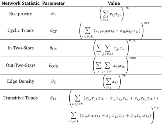
Network Statistic Parameter Value
Reciprocity θR
˜ ÿ
iăj xijxji
¸αR
Cyclic Triads θCT
¨
˝ ÿ
iăjăk
pxijxjkxki`xikxkjxjiq
˛
‚
αCT
In-Two-Stars θITS
¨
˝ ÿ
i
ÿ
jăk‰i xjixki
˛
‚
αITS
Out-Two-Stars θOTS
¨
˝ ÿ
i
ÿ
jăk‰i xijxik
˛
‚
αOTS
Edge Density θE
˜ ÿ
i‰j xij
¸αE
Transitive Triads θTT
¨
˝ ÿ
iăjăk
pxijxjkxik`xijxkjxki`xijxkjxikq `
ÿ
iăjăk
pxjixjkxki`xjixjkxik`xjixkjxkiq
˛
‚
αTT
Table 1: Summary of network statistics used in the specification of a GERGM in this work. These are theα-outside specification of five commonly-used network statistics.
one can easily identify non-degenerate GERGM specifications for a weighted version of the
two-star model. Importantly, we show that under certain weightings, Metropolis–Hastings
can simulate networks with any desired edge density and clustering structure. The R code
and all of the data used in this section are available in the online supplement.
5.1
International Lending Network
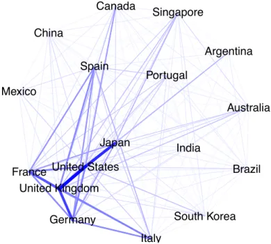
Our first application of the GERGM is to the network of aggregate private and public lending
between 17 large industrialized nations in 2005. Weighted directed edges between nations
represent the total monetary volume, in millions of U.S. dollars, that was loaned from one
nation to another. Figure1illustrates this weighted network. This data was collected by the
Bank for International Settlements (BIS) and a descriptive analysis was originally published
inOatley et al.(2013). To the best of our knowledge, there have been no published studies
exploratory, and descriptive analyses on international lending as a network phenomenon
(Niemira and Saaty, 2004; Nier et al., 2007; Rodriguez, 2007; Gai and Kapadia, 2010;
Amini et al.,2013;Billio et al.,2012), especially in the wake of the 2008 financial crisis.
One particular challenge in this network is the heavy tailed nature of the lending volumes
(with the majority of lending concentrated between Germany, Great Brittan, Japan, and
the United States). We first apply an ln(x+1) transformation on all aggregate lending
flows between countries - a standard practice in international finance applications - and
subsequently model the transformed edge weights using the GERGM.
Argentina
Australia
Brazil Canada
China
France
Germany
India
Italy Japan
South Korea Mexico
Portugal Singapore
Spain
United Kingdom United States
Edge Values
0 1173.32
Figure 1: Network plot of the international aggregate interbank lending network. Darker edges indicate a larger volume of lending.
We control for several important exogenous predictors in the GERGM specification. In
particular, we include sender and receiver effects for the (natural log) gross domestic
prod-uct (GDP) as we expect countries with larger economies to both lend and borrow more
than those with smaller economies. We also include network predictors that represent
(nor-malized) aggregate trade volume between countries, as well as the (nor(nor-malized) number
of inter-governmental organization (IGO) co-memberships. We expect that countries that
trade more with one another will also lend more with one another, and that those countries
more frequently with one another due to their increased diplomatic cooperation. Finally,
we include mixing matrices parameterizing the propensity for countries to lend to each
other based on G8 membership2. We choseT as the cdf of a Student’st distribution with
one degree of freedom, whose median is a linear regression on the specified exogenous
predictors.
In addition to the exogenous predictors discussed above, we also include structural
network predictors, including mutual dyads, transitive triads, and out two-stars statistics
in our model. These statistics allow us to test for the presence of mutuality, clustering, and
economies of scale in lending, all of which are theoretically important in the international
trade (Oatley et al.,2013). Although this specification includes a number of exogenous
covariates for control, we find that GERGM model with no α down weighting exhibited
degeneracy. To address this degeneracy, we considered an exponentially weighted model
using statistics from Table1. We used the Metropolis–Hastings procedure to estimate the
GERGM where network predictors were down-weighted by αR “ αTT “ αOTS “ 0.8. The 0.8 value was selected because it was the lagest value for which we could consistently
estimate a non-degenerate model across multiple runs of estimation. We optimized the
Metropolis-Hastings proposal variance at each step in the estimation process (with a target
acceptance rate of 0.25˘0.05) initialized a burn-in of 400,000 full network samples, and then sampled 800,000 networks from which we thinned the resulting sample by keeping
every two hundredth network. The average acceptance rate was approximately 0.22. The
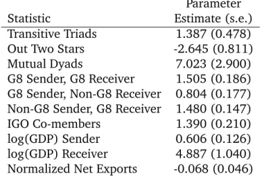
resulting parameter estimates are given in Table2. To assess convergence of the estimated
models, we simulated 800,000 networks and compared the distribution of the mutual dyads,
transitive triads, and out two-stars statistics to the observed values in the lending network.
Further, we investigated the goodness of fit of our model by comparing the distributions of
the simulated and observed in two-stars, cyclic triads, and network density distributions.
These results are shown in Figure2.
As we can see from Figure 2, our model has appeared to have converged based on the
distributions of the transitive triads, mutual dyads, and out two-stars statistics. In terms of
goodness of fit, we see that our model provides a very good fit for the observed network in
2The G8 member countries are Canada, France, Germany, Italy, Japan, Russia, the United Kingdom and
Parameter
Statistic Estimate (s.e.)
Transitive Triads 1.387 (0.478)
Out Two Stars -2.645 (0.811)
Mutual Dyads 7.023 (2.900)
G8 Sender, G8 Receiver 1.505 (0.186) G8 Sender, Non-G8 Receiver 0.804 (0.177) Non-G8 Sender, G8 Receiver 1.480 (0.147)
IGO Co-members 1.390 (0.210)
log(GDP) Sender 0.606 (0.126)
log(GDP) Receiver 4.887 (1.040)
Normalized Net Exports -0.068 (0.046)
Table 2: Estimates of the network parameters of the GERGM model when fit to the international lending network via the Metropolis–Hastings procedure.
terms of cyclic triads; however, the in-two-stars and network density values are somewhat
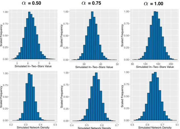
overestimated. Geweke statistics and trace plots of the network density for 800,000
net-works simulated from the fitted GERGM specification via Metropolis–Hastings simulation
also indicate that the model has converged (see Figure6in the Appendix). The exogenous
covariate parameter estimates from our model largely conform to our theoretical
expecta-tion, although it is interesting that we see a small (negative) parameter estimate for the
effect of trade, indicating that there is not a particularly strong relationship between trade
and lending in our network, when controlling for other economic and network factors. We
observe positive and statistically significant transitivity and reciprocity effects, and a
nega-tive out-two stars effect. These results are interesting because previous studies, including
Oatley et al.(2013), have argued that the international lending network is hierearchical
-a property th-at does not m-atch our results -as we would expect to see -a positive out
two-stars parameter estimate. Further exploration of this finding is outside of the scope of this
discussion, but should be considered in future research.
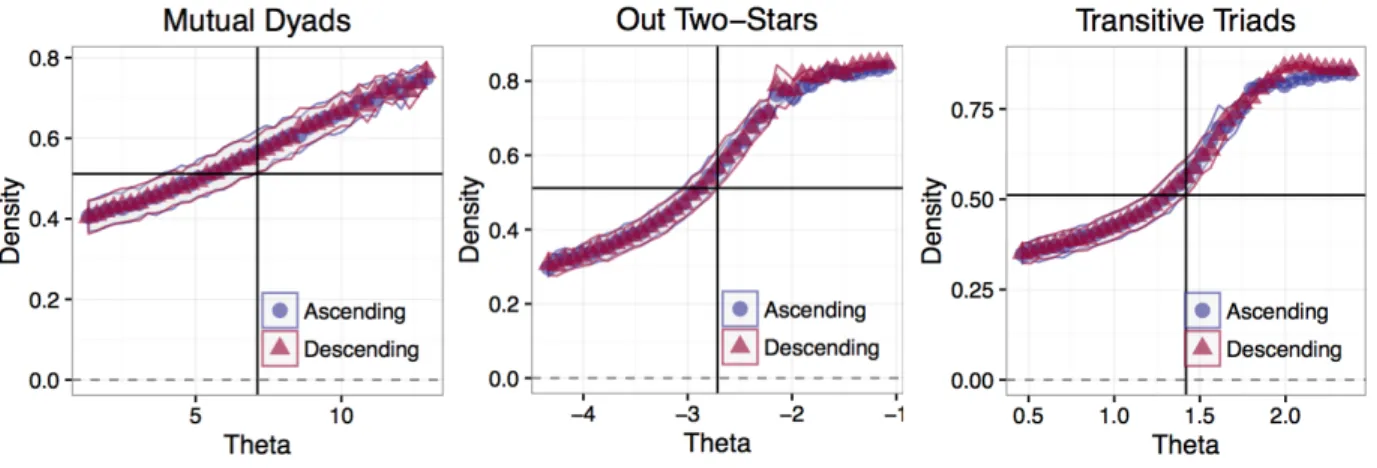
To further asses the potential for degeneracy in our model, we performed a hysteresis
analysis similar to that described in Snijders et al. (2006) for each structural parameter
estimate. Starting with a sparse network and holding all other parameter estimates at their
posterior means, we varied each structural parameter estimate ten standard deviations
below to ten standard deviations above its posterior mean and simulated 500,000 networks
−3 −2 −1 0 1 2 3 4
Blue = Observed Statistic, Red = Simulated Mean
Nor
maliz
ed Statistic V
alues
Out 2−Stars
In 2−Stars
Cyclic Triads
Mutual Dyads
Transitive Triads
Network Density
Figure 2:Convergence and goodness of fit plots for the model fitted to the international lending network. For each fit model, 800,000 networks were simulated using the Metropolis–Hastings sampling procedure and the final exogenous and structural parameter estimates. Each box plot compares the quantiles of simulated networks (with mean statistic values at the red line) to the observed network statistic (blue line). Here, the In 2-Stars and Network Density statistics were not included in the fitted model.
a burnin of 500,000). We changed the structural parameter value 0.5 standard deviations
at each iteration of this process, for a total of 41 parameter values. For each new value
of the parameter, we used the final network from the M-H simulation using the previous
parameter value as the initialization for the M-H simulation for the new specified parameter.
We plotted the mean network density against the parameter values in order to asses the
potential for jumps in the network density that might indicate an underlying issue with
model degeneracy. Figure 3 shows the hysteresis plots for our model, and these plots do
not indicate any obvious issues with degeneracy in this specification.
5.2
U.S. Migration Network
We next apply the GERGM to the U.S. migration network analyzed inDesmarais and
Cran-mer(2012). We note that this application is used for validation of our Metropolis–Hastings
procedure; indeed, we compare the estimates obtained with Metropolis–Hastings directly
with the estimates obtained from the Gibbs sampler for the same GERGM specification.
Historically, interstate migration has played an important role in the understanding of
local financial markets, public infrastructure, and the political climate within each state
Figure 3:Hysteresis plots for the international trade network. Shaded regions cover˘1.96standard deviations in the simulated network densities for that parameter value. The vertical black line indicates the parameter value from the main estimation step and the horizontal black line indicates the observed network density.
The network that we model contains 51 nodes that represent the 50 U.S. states as well as
Washington, D.C. Directed edges are placed between states in which there was a change in
interstate migration flow from 2006 and 2007. The weight,yij, associated with the directed edge from nodeito nodej is the total change in interstate migration from stateito statej
between 2006 to 2007. This data set also contains ten demographic exogenous predictors
that further describes the pairwise relationships between states. The predictors describe
the geographic distance, and the sender and receiver effects of high January temperature,
income, unemployment, and population of the states. Like the application in Section 5.1,
we choseT as the cdf of a Student t distribution with one degree of freedom, whose median
is a linear regression on the specified demographic predictors.
We incorporated network statistics that represent reciprocity, cyclic triads, in-two-stars,
out-two-stars, and transitive triads in our GERGM specification, and following the model
fit inDesmarais and Cranmer (2012) we used noα down-weighting.
We fit the above model using both the Metropolis–Hastings sampling procedure and
Gibbs. For Gibbs, we use 50,000 simulated networks with a set burn-in of 10,000 networks
in each iteration. We optimized the Metropolis-Hastings proposal variance at each step
in the estimation process (with a target acceptance rate of 0.25) initialized a burn-in
we thinned the resulting sample by keeping every one thousandth network. The average
acceptance rate was approximately 0.24. The parameter estimates and associated standard
errors for each method are shown on in Table3.
M-H Parameter Gibbs Parameter
Statistic Estimate (s.e.) Estimate (s.e.)
Transitive Triads 0.074 (0.053) 0.078 (0.053)
Cyclic Triads -0.206 (0.042) -0.204 (0.040)
Out Two Stars 0.017 (0.044) 0.011 (0.043)
In Two Stars -0.029 (0.039) -0.030 (0.040)
Mutual Dyads -0.131 (0.348) -0.107 (0.338)
Unemployment Sender 27.163 (13.481) 27.402 (13.463) Unemployment Receiver -3.673 (12.382) -3.475 (12.476) Mean January Temp. Sender -11.031 (14.474) -11.167 (14.452) Mean January Temp. Receiver -15.147 (13.609) -15.101 (13.713) Population Size Sender 1.806 (20.264) 1.744 (20.244) Population Size Receiver -35.532 (16.127) -35.282 (16.215)
Mean Income Sender 2.349 (11.613) 2.220 (11.583)
Mean Income Receiver -1.129 (10.652) -0.969 (10.735)
Distance 7.081 (11.917) 7.218 (11.970)
Dispersion 5.942 (0.029) 5.942 (0.029)
Table 3: Estimates of the network parameters of the GERGM model when fit to the U.S. migration network via the Metropolis–Hastings and Gibbs sampler procedures.
Table3reveals that the Metropolis–Hastings and Gibbs procedures provide comparable
estimates for each of the modeled predictors. This suggests that each method simulates
from the same distribution, as expected. Furthermore, these fitted GERGM reveals three
interesting, perhaps expected, trends in the data: (i) there was increased migration away
from states with high unemployment, (ii) there was decreased migration to states with a
large population, and (iii) there was decreased migration to states with high
unemploy-ment. See Desmarais and Cranmer(2012) for a more detailed discussion of these results.
We provide further estimation diagnostics for the Metropolis–Hastings procedure in the
Appendix.
5.3
Non-Dengenerate Specifications of the Two-Star Model
In our simulation study, we consider fitting a GERGM to a directed and weighted variant of
ofxas a function of its edges and in-two-stars:
fXpx, θθθ, αq “
exppθEhEpxq `θITShIT Spx, αqq CpθE, θITSq
, xP r0,1sm (16)
hEpxq “
ÿ
i‰j xij{m
hIT Spx, αq “
˜ ÿ
i
ÿ
jăk‰i xjixki
¸α ,
whereCpθE, θITSqis the normalizing constant that ensuresfXpx, θθθqintegrates to one,hEpxq is the edge density ofx, andhIT Spx,1qis the in-two-star density ofx. Whenα“1, model (16) is the directed and weighted version of the two-star model considered in Handcock
et al. (2003). Model (16) is closely related to the triangle model fromJonasson (1999);
H¨aggstr¨om and Jonasson(1999) and the widely used Ising model for lattice processes. We
will refer to model (16) as the weighted in-two-stars model.
The unweighted two-star model is a well-known example that suffers from likelihood
degeneracy (see Handcock et al. (2003) or Snijders et al. (2006) for instance). In this
simulation study, we empirically analyze model (16) following a similar study as that
described in Snijders et al. (2006). We find that, surprisingly, the weighted in-two-stars
model doesnotdemonstrate the typical signs of degeneracy. We now describe the simulation
study and our findings.
We first fix the edge density parameterθE at -2 and a value ofα between 0 and 1. We then simulate one million size 10 networks following model (16) for each integer value of
θITS between -10 and 10 using the MH sampler. We calculate the mean edge density and
the mean in-two-stars value from the million samples at each value ofθITS. We repeat this
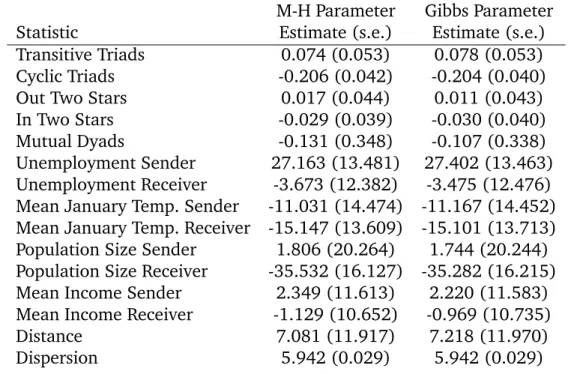
procedure forα values of 0.10, 0.25, 0.50, 0.75, 0.90, and 1. The results are reported in
Figure4.
We see from Figure 4 that forα “ 1, there is a large jump in the value of the in-two-stars and edge density statistics betweenθITS“0andθITS “1. Asαdecreases, the relative magnitude of this jump decreases and the statistics’ curves are relatively smooth over
0.0 0.2 0.4 0.6 0.8 1.0
−
10 −9 −8 −7 −6 −5 −4 −3 −2 −1 0 1 2 3 4 5 6 7 8 9 10
α 0.1 0.25 0.5 0.75 0.9 1 0
50 100 150 200 250 300 350
−
10 −9 −8 −7 −6 −5 −4 −3 −2 −1 0 1 2 3 4 5 6 7 8 9 10 α
0.1 0.25 0.5 0.75 0.9 1
In-Two-Stars
Edge Density
Figure 4:The mean value of the in-two-stars statistic and the edge density of one million simulated networks of the in-two-stars model with θE “ ´2and integer values of θITS from -10 to 10. The
mean values are shown forα values of 0.10, 0.25, 0.50, 0.75, 0.90, and 1.
one and the edge density only changes slightly across values ofθITS. The jump phenomenon
was also witnessed for binary networks in the two-stars model in Snijders et al. (2006),
where it was observed that this model specification was most prone to degeneracy issues.
As a consequence, one may expect the empirical distribution of the in-two-stars and
edge-density statistics in the neighborhood ofθITS “0andθITS“1to be bimodal at large values ofα.
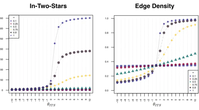
To investigate whether this is the case, we performed a more fine grained grid search
for the value ofθITSat which the edge density of the network changed the most, for each
value of α. We found that, for example, when α “ 0.5, the steepest change in the edge density occurred at approximately θIT S “ 0.55. Similarly, for α “ 0.75 and α “ 1, the steepest changes in the edge density occurred at approximatelyθIT S “0.65andθIT S “0.75, respectively. We show the empirical distribution for both of the statistics for α values of
these distributions arenotbimodal for these values ofα, includingα“1. We also evaluated these distributions for all other values ofθITS in our simulations and found similar results.
Furthermore, these results are not sensitive to the value of θE, as it serves only to shift the curves depicted in Figure 4 left or right. These findings suggest that the weighted
in-two-stars does not suffer from the same degeneracy issues as its binary counterpart.
0.00 0.25 0.50 0.75 1.00
80 120 160 200
Simulated In−Two−Stars Value
Scaled Frequency
= 0.50 = 0.75 = 1.00
0.00 0.25 0.50 0.75 1.00
30 40 50
Simulated In−Two−Stars Value
Scaled Frequency 0.00 0.25 0.50 0.75 1.00
5 6 7 8
Simulated In−Two−Stars Value
Scaled Frequency 0.00 0.25 0.50 0.75 1.00
0.5 0.6 0.7 0.8
Simulated Network Density
Scaled Frequency 0.00 0.25 0.50 0.75 1.00
0.4 0.5 0.6 0.7
Simulated Network Density
Scaled Frequency 0.00 0.25 0.50 0.75 1.00
0.2 0.3 0.4 0.5
Simulated Network Density
Scaled Frequency
Figure 5: The empirical (scaled) frequency distribution of the edge density and the in-two-stars value for the in-two-stars model atθITS“ t0.55,0.65,0.75u(from left to right). One million networks
were simulated and the values for each statistic is shown over all networks.
In summary, this simulation study provides insights into two important features of the
GERGM specification of the two-stars model. First, the weighted in-two-stars models does
not appear to suffer from degeneracy at any value ofα. This surprising result is contrary to
the well-known unweighted two-stars model. This simulation also gives some intuition as
to how to choose the tuning parameterα. Small values ofα(ď0.50) dampened the effect of the in-two-stars statistic too drastically and are therefore not suggested. We encourage
GERGM model to parameter changes.
6
Discussion
We have proposed, explicated, and demonstrated several advances in the statistical
mod-eling of weighted networks by substantially increasing the utility of the GERGM. These
extensions to the GERGM, taken together, represent a significant increase in the model’s
capabilities, such that it is now possible to use nearly any model specification for inference
on continuous-valued weighted graphs.
First, we have proposed and implemented a Metropolis–Hastings algorithm for fitting
GERGMs. In the original development of the GERGM, Desmarais and Cranmer (2012)
proposed a Gibbs sampling strategy to estimate the model. However, this approach is
limited by the fact that fairly strict constraints are placed on the set of network statistics
that can be used in the model. Our Metropolis–Hastings procedure relaxes these restrictions
and allows one to use the full set of possible specifications for the model.
Second, we have proposed an approach to dampening the extreme values often
pro-duced by subgraph sums and thus avoiding model degeneracy. This dampening technique,
because it is critical in avoiding degenerate model specifications in the GERGM, allows
ana-lysts to specify a practical and diverse set of endogenous effects as part of the network data
generating process. Though this may seem a simple extension to the means by which
statis-tics are computed on the network, this weighting strategy is important because degeneracy
is a major obstacle to estimation of inferential models on real-world networks.
We consider two approaches to network statistic dampening—one in which
subgraph-specific sums are raised to a fractional exponent (i.e.,α-inside dampening), and a stronger
approach that involves raising the sum over all subgraphs to a fractional exponent (i.e.,
α-outside dampening). It is important to re-iterate that, while the α-inside approach
con-forms to the local dependence that is typical to ERGM formulations, theα-outside approach
induces global dependence in that each tie variable depends to some degree on the value of
every other tie variable in the network. We see from Equation15that theα-outside
formu-lation exhibits a form of dependence similar to theα-inside formulation in that high edge
and associated with positive parameter values. However, theα-outside formulation exhibits
an additional form of dependence in that the likelihood of high edge values embedded in
high value configurations decreases as the global sum over the respective configuration
type increases. This global dampening in the α-outside model is inversely related to the
value of α. Though the α-inside and α-outside formulations may both be considered in
efforts to avoid degeneracy, we note that researchers should also consider how the choice
between these two formulations affects the interpretation of results.
Though we have presented important innovations here, much work remains. Specifically,
we have just scratched the surface when it comes to model selection and specification for
GERGMs. First, both inDesmarais and Cranmer(2012) and in the current study, the
statis-tics used to specify the GERGM have represented straightforward functional adaptations
of the statistics commonly used for binary ERGMs. Future research should consider suites
of statistics that are applicable to the special case of weighted networks. Furthermore, our
approach to weighting the subgraph products requires a choice ofαthat will rarely be
theo-retically informed. In our simulation study, we analyzed the effects ofαon the sensitivity of
the two-stars model and found encouraging results forα P p0.5,1s. In principle, one could use an alternative data-driven approach that choosesαbased on goodness of fit summaries.
We plan to investigate this more fully in future work. Finally, the results in the simulation
study gave empirical evidence in one well-studied model that the GERGM does not suffer
from degeneracy like its binary ERGM counterpart. We aim to theoretically formalize these
Appendix
A: Pseudo-code for MCMC Maximum Likelihood Estimation of the GERGM
Algorithm 1: G E R G M M C M C M L E
Data: Data and parameters yÐvector of edge weights
Tol1Ðtolerance level for GERGM estimation convergence
Tol2Ðtolerance level for Metropolis–Hastings algorithm convergence
NÐnumber of network samples generated for each iteration of Metropolis–Hastings sampler hÐvector of functions to calculate network statistics
TÐtransformation function
cÐshape parameter # Default = 1
tÐ0 # iteration number
∆1Ð1000
∆2Ð1000
while∆1ąTol1do
t++; # Increment iteration
ift = 1then
ES T I M AT E βtvia MPLE
else
ES T I M AT E βtvia Gradient Descent
ES T I M AT E TH E TA viaAlgorithm 2to obtainθt
end
if}βt´1}22}θt´1}22ą0then
∆1“ 12
„
}βt´βt´1}22 }βt´1}22
`}θt´θt´1} 2 2 }θt´1}22
else
∆1“ 12
“
}βt´βt´1}22` }θt´θt´1}22
‰
end end
Algorithm 2: ES T I M AT E TH E TA
# Initialize parameters
ˆ
x“Tpy, βtq # current estimate of edge weights based on estimate ofβt ˜
θ0“θt´1 # initialization of coefficient vector r = 0 # iteration number
m = length(y) # Number of edges
while∆2ąTol2do
r++ # Increment iteration
Simulate a samplex0of lengthmfrom density:
fpx|θ˜r´1q “ exprθ˜1
r´1hpxqs
Cpθ˜0q
, Cpθ˜r´1q “ ż
r0,1sM
exprθ˜1
r´1hpzqsdz
RU N ME T R O P O L I S HA S T I N G S UP D AT E viaAlgorithm 3to obtain samplesx1, . . . , xN.
# Updateθ˜r ˜
θr“argmaxθ ”
θ1h
pxˆq ´logrCppθqs ı
via Gradient Descent, where
p
Cpθq “ Cp
˜ θr´1q
N N ÿ
j“1
exprpθ´θr˜´1q1hpxjqs
# Calculate distance from previous step
if}θr˜´1}22ą0then
∆2“
}θr˜ ´θr˜´1}22
}θ˜r´1}22
else
∆2“ }θr˜ ´θr˜´1}22
Algorithm 3: ME T R O P O L I S HA S T I N G S UP D AT E
Data: Data and Parameters
σ2: variance of Truncated Normal density # Default = 1
x0Initial weighted network sample (all edges have values between 0 and 1.
n: total number of nodes in the network
# loop over number of MH network samples
fork = 0; kăN; k++do
# Draw a single proposal sample
fori = 0; iăn; i++do forj = 0; jăn; j++do
Sample a proposed edge weightwijfrom a truncated normal distribution centered at the previous iteration’s edge weight
wij „T N`xk´1
ij , σ
2˘
Calculate the probability of the proposed edge weightwij under the truncated normal distribution centered around the current edge weight (xkij´1).
ppwqij “P`wďwij |xk´1
ij , σ
2˘
Calculate the probability of the current edge weight (xk´1
ij ) under a truncated normal
distribution centered around the proposed edge weight (wij).
ppxqij “P`wďxk´1
ij |wij, σ
2˘
end end
Setwas the proposed network andxk´1as the previous iteration’s network. Calculate the following log joint pdfs:
Px“ n ÿ i n ÿ j
logpppxqijq
Pw“ k ÿ i k ÿ j
logpppwqijq
Calculateα“ pPx´Pwq `θ1 “
hpwijq ´hpxkij´1q ‰
Sampleufrom a Uniform(0,1) density
iflogpuq ďαthen
xk“w
else
xk“xk´1
end end
returnx1, . . . , xN
B: GERGM Fit Diagnostics
6. For the U.S. Migration data, we simulated 100,000 networks with 10,000 burn-in. The modeled statistics, as well as the MCMC traceplot for the network density for this data are shown in Figure7. Visual inspection as well as the Geweke convergence test statistic suggest that the sampler has converged.
Figure 6:International lending network trace plot for the network density of the simulated networks over 800,000 simulations from Metropolis–Hastings.
References
Amini, H., Cont, R. and Minca, A. (2013), ‘Resilience to contagion in financial networks’,
Mathematical Financepp. 1–40.
Billio, M., Getmansky, M., Lo, A. W. and Pelizzon, L. (2012), ‘Econometric measures of connectedness and systemic risk in the finance and insurance sectors’,Journal of Financial Economics104(3), 535–559.
Browne, W. J. (2006), ‘Mcmc algorithms for constrained variance matrices’,Computational Statistics & Data Analysis50(7), 1655–1677.
Chatterjee, S., Diaconis, P. et al. (2013), ‘Estimating and understanding exponential random graph models’,The Annals of Statistics 41(5), 2428–2461.
Chun, Y. (2008), ‘Modeling network autocorrelation within migration flows by eigenvector spatial filtering’,Journal of Geographical Systems10(4), 317–344.
Claeskens, G., Silverman, B. W. and Slaets, L. (2010), ‘A multiresolution approach to time warping achieved by a bayesian prior–posterior transfer fitting strategy’,Journal of the Royal Statistical Society: Series B (Statistical Methodology)72(5), 673–694.
Clark, G. and Ballard, K. (1981), ‘The demand and supply of labor and interstate relative wages: an empirical analysis’,Economic Geographypp. 95–112.
Desmarais, B. and Cranmer, S. (2012), ‘Statistical inference for valued-edge networks: The generalized exponential random graph model’,PLoS ONE7(1), e30136.
Frank, O. and Strauss, D. (1986), ‘Markov graphs’,Journal of the American Statistical Asso-ciation81(395), 832–842.
Franks, A. M., Cs´ardi, G., Drummond, D. A. and Airoldi, E. M. (2014), ‘Estimating a struc-tured covariance matrix from multi-lab measurements in high-throughput biology’, Jour-nal of the American Statistical Association(just-accepted), 00–00.
Gai, P. and Kapadia, S. (2010), ‘Contagion in financial networks’,Proceedings of the Royal Society A: Mathematical, Physical and Engineering Sciences466(2120), 2401–2423.
Genest, C. and MacKay, J. (1986), ‘The joy of copulas: Bivariate distributions with uniform marginals’,The American Statistician40(4), 280–283.
Geweke, J. (1991),Evaluating the accuracy of sampling-based approaches to the calculation of posterior moments, Vol. 196, Federal Reserve Bank of Minneapolis, Research Department.
Geyer, C. and Thompson, E. (1992), ‘Constrained monte carlo maximum likelihood for dependent data’,Journal of the Royal Statistical Society. Series B (Methodological)pp. 657– 699.
H¨aggstr¨om, O. and Jonasson, J. (1999), ‘Phase transition in the random triangle model’,
Journal of Applied Probabilitypp. 1101–1115.
Handcock, M. S., Robins, G., Snijders, T., Moody, J. and Besag, J. (2003), ‘Assessing degener-acy in statistical models of social networks’,Journal of the American Statistical Association
76, 33–50.
Holland, P. and Leinhardt, S. (1981), ‘An exponential family of probability distributions for directed graphs’,Journal of the American Statistical Association76(373), 33–50.
Hunter, D. and Handcock, M. (2006), ‘Inference in curved exponential family models for networks’,Journal of Computational and Graphical Statistics15(3), 565–583.
Hunter, D. R., Handcock, M. S., Butts, C. T., Goodreau, S. M. and Morris, M. (2008), ‘ergm: A package to fit, simulate and diagnose exponential-family models for networks’,Journal of Statistical Software24(3), 1–29.
Iori, G., De Masi, G., Precup, O., Gabbi, G. and Caldarelli, G. (2008), ‘A network analy-sis of the italian overnight money market’, Journal of Economic Dynamics and Control
32(1), 259–278.
Jonasson, J. (1999), ‘The random triangle model’, Journal of Applied Probabilitypp. 852– 867.
Krivitsky, P. N. (2012), ‘Exponential-family random graph models for valued networks’,
Electronic Journal of Statistics6, 1100–1128.
Levine, P. and Zimmerman, D. (1999), ‘An empirical analysis of the welfare magnet debate using the nlsy’,Journal of Population Economics 12(3), 391–409.
Lubetzky, E. and Zhao, Y. (2014), ‘On replica symmetry of large deviations in random graphs’,Random Structures & Algorithms.
Lubetzky, E. and Zhao, Y. (2015), ‘On replica symmetry of large deviations in random graphs’,Random Structures & Algorithms47(1), 109–146.
M¨uller, G. (2010), ‘Mcmc estimation of the cogarch (1, 1) model’, Journal of Financial Econometrics8(4), 481–510.
Neelon, B., Anthopolos, R. and Miranda, M. L. (2014), ‘A spatial bivariate probit model for correlated binary data with application to adverse birth outcomes’,Statistical methods in medical research23(2), 119–133.
Niemira, M. P. and Saaty, T. L. (2004), ‘An Analytic Network Process model for financial-crisis forecasting’,International Journal of Forecasting20(4), 573–587.
Oatley, T., Winecoff, W. K., Pennock, A. and Danzman, S. B. (2013), ‘The Political Economy of Global Finance: A Network Model’,Perspectives on Politics11(01), 133–153.
Park, J. and Newman, M. (2004a), ‘Solution of the two-star model of a network’,Physical Review E70(6), 066146.
Park, J. and Newman, M. (2004b), ‘Statistical mechanics of networks’,Physical Review E
70(6), 66117–66130.
Park, J. and Newman, M. E. (2004c), ‘Solution of the two-star model of a network’,Physical Review E70(6), 066146.
Pattison, P. and Robins, G. (2002), ‘Neighborhood-based models for social networks’, Socio-logical Methodology32, 301–337.
Rinaldo, A., Fienberg, S. and Zhou, Y. (2009), ‘On the geometry of discrete exponential families with application to exponential random graph models’, Electronic Journal of Statistics3, 446–484.
Roberts, G. O., Gelman, A. and Gilks, W. R. (1997), ‘Weak convergence and optimal scaling of random walk metropolis algorithms’,The annals of applied probability7(1), 110–120.
Robins, G., Pattison, P. and Wasserman, S. (1999), ‘Logit models and logistic regressions for social networks: Iii. valued relations’,Psychometrika64(3), 371–394.
Rodriguez, J. C. (2007), ‘Measuring Financial Contagion: A Copula Approach’,Journal of Empirical Finance14(3), 401–423.
Schweinberger, M. (2011), ‘Instability, sensitivity, and degeneracy of discrete exponential families’,Journal of the American Statistical Association106(496), 1361–1370.
Simpson, S. L., Hayasaka, S. and Laurienti, P. J. (2011), ‘Exponential random graph model-ing for complex brain networks’,PLoS ONE6(5), e20039.
Snijders, T. A. B. (2002), ‘Markov chain monte carlo estimation of exponential random graph models’,Journal of Social Structure3(2), 1–40.
Snijders, T., Pattison, P., Robins, G. and Handcock, M. (2006), ‘New specifications for expo-nential random graph models’,Sociological Methodology36(1), 99–153.
Snyman, J. (2005),Practical mathematical optimization: an introduction to basic optimiza-tion theory and classical and new gradient-based algorithms, Vol. 97, Springer Science & Business Media.
Strauss, D. and Ikeda, M. (1990), ‘Pseudolikelihood estimation for social networks’,Journal of the American Statistical Association85(409), 204–212.
Wasserman, S. and Pattison, P. (1996), ‘Logit models and logistic regressions for social networks: I. an introduction to markov graphs andp˚’,Psychometrika61(3), 401–425.