arXiv:1607.07877v2 [astro-ph.CO] 8 Dec 2016
Carisa Miller∗ and Adrienne L. Erickcek†
Department of Physics and Astronomy, University of North Carolina at Chapel Hill, Phillips Hall CB3255, Chapel Hill, North Carolina 27599, USA
In chameleon gravity, there exists a light scalar field that couples to the trace of the stress-energy tensor in such a way that its mass depends on the ambient matter density, and the field is screened in local, high-density environments. Recently it was shown that, for the runaway potentials commonly considered in chameleon theories, the field’s coupling to matter and the hierarchy of scales between Standard Model particles and the energy scale of such potentials result in catastrophic effects in the early Universe when these particles become nonrelativistic. Perturbations with trans-Planckian energies are excited, and the theory suffers a breakdown in calculability at the relatively low tem-peratures of Big Bang Nucleosynthesis. We consider a chameleon field in a quartic potential and show that the scale-free nature of this potential allows the chameleon to avoid many of the problems encountered by runaway potentials. Following inflation, the chameleon field oscillates around the minimum of its effective potential, and rapid changes in its effective mass excite perturbations via quantum particle production. The quartic model, however, only generates high-energy perturba-tions at comparably high temperatures and is able remain a well-behaved effective field theory at nucleosynthesis.
I. INTRODUCTION
Many explanations for the current accelerated expan-sion of the Universe posit the existence of a new light scalar field. These scalar fields are usually coupled to matter and so can mediate long-range forces, often of gravitational strength. Such scalars are not only cos-mologically motivated, but also pervasive in high-energy physics and string theory. However, stringent experimen-tal bounds imply tight constraints on any new fifth forces mediated by scalar fields. These constraints require the scalar’s coupling to matter to be tuned to unnaturally small values in order to avoid detection. Another ap-proach is to employ a screening mechanism, which sup-presses effects of the field locally, allowing consistency with successful tests of general relativity.
One of the few known screening mechanisms capable of reconciling the predictions of scalar-tensor gravitational theories and experimental constraints is the chameleon mechanism [1, 2]. In chameleon gravity theories, the scalar field’s potential function and its coupling to the stress-energy tensor combine into an effective potential whose minimum is dependent on the matter density of its environment. Consequently, the effective mass of the chameleon field is also dependent on the environment, in-creasing enough in regions of high density to suppress the field’s ability to mediate a long-range force. Because of this ability to hide within its environment, the chameleon can couple to matter with gravitational strength and still evade experimental detection in laboratory and Solar System tests of gravity.
The vast majority of cosmological investiga-tions of chameleon gravity have considered
po-∗Electronic address: [email protected] †Electronic address: [email protected]
tentials of the runaway form, such as the ex-ponential V(φ) =M4exp[(M/φ)n] and power-law
V(φ) = M4+nφ−n potentials. In order to evade Solar System tests of gravity, M has to be set to a value of ∼10−3 eV, which is the energy scale of dark energy [2].
This coincident energy scale gave the chameleon a lot of attention early on as a possible explanation for cosmic acceleration. However, it was shown in Ref. [3] that the chameleon field cannot account for the accelerated expansion of the Universe without including a constant term in its potential. Nevertheless, light scalar fields arise in many theories that consider physics beyond the Standard Model (SM), and the chameleon mechanism remains one of the most-studied approaches to screening the unwanted forces mediated by these fields.
analy-ses focus specifically on potentials of the power-law form. Given the tremendous experimental effort under way to detect or constrain chameleons, it is troubling that the most widely studied chameleon models have been shown to suffer a breakdown in calculability in the early Uni-verse due to the discrepancy between the chameleon mass scale and that of the SM particles [20, 21].
We aim to identify a chameleon potential that can avoid the computational breakdown suffered by runaway models. We analyze a class of potential not often con-sidered in chameleon theories: the quartic potential, V(φ) = κφ4/4!. Prevalent in high-energy theories, the
quartic potential is also viable as a chameleon model be-cause the self-interaction of this potential is sufficient to ensure that the field will be adequately screened in high-density environments [22]. The scale-free property of the quartic model is potentially beneficial as it can avoid the hierarchy of energy scales that arises due to the low-energy scale of the runaway potentials, and we investigate whether it is able to remain well-behaved in the early Universe.1
In runaway chameleon models, the field rolls to some value far from the minimum of its effective potential after inflation and remains stuck there during the radiation-dominated era due to Hubble friction. The chameleon’s coupling to the trace of the stress-energy tensor makes it sensitive to the energy density,ρ, and pressure,P, of the radiation bath through the quantity Σ≡(ρ−3P)/ρ. While the Universe is radiation dominated, Σ is nearly zero and the chameleon is light enough that Hubble fric-tion is able to prevent it from rolling toward its poten-tial minimum. However, as the temperature of the ra-diation bath cools, particle species in thermal equilib-rium become nonrelativistic and Σ momentarily becomes nonzero. The chameleon then gains mass, is able the overcome Hubble friction, and is seemingly “kicked” to-ward the minimum of its effective potential [24].
Originally, the kicks were seen as an auspicious way to bring runaway chameleons to their potential mini-mum prior to Big Bang Nucleosynthesis (BBN).2
How-ever, they impart such a high velocity to the field that the chameleon rebounds off the other side of its effective potential back to field values further from the potential minimum than where it was stuck when the kick began
1 Another proposed way to avoid the detrimental effect of the kicks is to include DBI-inspired corrections to the chameleon’s Lagrangian that weaken the chameleon’s coupling to matter at high energies. This modification effectively introduces a sec-ond screening mechanism analogous to a Vainshtein screening in which derivative interactions weaken the effect of the kicks [23].
2 A consequence of the chameleon’s coupling to matter is that
any variation in the chameleon field can be recast as a variation in particle masses in the Jordan frame. As we know particle masses differed very little between BBN and the present day, this constrains the chameleon to be at or near the minimum of its potential prior to the onset of BBN [24].
[25]. However, Ref. [25] also showed that the inclusion of a coupling between the chameleon and the electromag-netic field offers a solution. The chameleon’s coupling to a primordial magnetic field allows the chameleon to overcome Hubble friction and begin oscillating about its potential minimum prior to the kicks. For a sufficiently rapidly oscillating field, the kicks then have little effect on the chameleon’s evolution.
These kicks further jeopardized chameleon theories by throwing into question their validity as a classical field theory [20, 21]. The effective potential in runaway mod-els is minimized whenφ∼M, and at field valuesφ.M, the extremely steep slope of the bare potential leads to rapid changes in the chameleon’s effective mass for small field displacements. Thus, the GeV-scale velocity with which the chameleon approaches its meV-scale minimum after the kicks causes nonadiabatic changes in the mass that excite extremely energetic fluctuations and lead to the quantum production of particles [20, 21]. Quan-tum corrections due to particle production then invali-date the classical treatment of the chameleon field and the particles’ trans-Planckian energies cast doubt on the chameleon’s viability as an Effective Field Theory (EFT) at the energy scale of BBN.
We will show that the quartic potential is able to avoid these problems due to its scale-free nature. In the early Universe, a chameleon field in a quartic potential oscil-lates rapidly with a large amplitude far beyond the mini-mum of its effective potential. In the classical treatment, the chameleon would continue this behavior until the end of radiation domination and still be oscillating far outside its minimum at the onset of BBN. A quantum treatment of the chameleon’s motion shows that these oscillations will create particles, albeit with much less energy than those created during the rebounds off runaway poten-tials. The same quantum effects that were catastrophic to previous chameleon models will cause the field to lose energy and bring the quartic chameleon to its potential minimum prior to the onset of the kicks. Consequently, for the quartic chameleon, these kicks do not have as sig-nificant an influence on the field’s evolution as in models with runaway potentials. Depending on the value ofκ, the rate at which the field loses energy can vary signif-icantly. For large values of κ, the field can lose all of its initial energy to particle production within the first oscillation and fall to its minimum. However whenκis closer to unity only a small percentage of the energy is lost during each oscillation, but the total effect accumu-lates over many oscillations to introduce a decay factor to the amplitude that still allows the field to reach its potential minimum before the kicks.
con-cluding remarks in Section V. Throughout this paper we will useMPl= (8πG)−1/2 andc=~= 1.
II. CLASSICAL CHAMELEONS
In theories of chameleon gravity, the action can be written as
S=
Z
d4x√−g∗
M2 Pl
2 R∗− 1 2(∇∗φ)
2
−V(φ)
+Sm[˜gµν, ψm], (1)
whereg∗is the determinant of the metricgµν∗ that solves the Einstein equations, R∗ is its Ricci scalar, andV(φ)
is the potential of the chameleon field,φ. The spacetime metric ˜gµνthat appears in the action for the matter fields,
Sm, governs geodesic motion and is conformally coupled to the Einstein metric by
˜
gµν =e−2βφ/MPl g∗µν, (2)
where β is a positive, dimensionless coupling constant assumed to be of order unity.3 This coupling implies
that the Einstein-frame stress-energy tensor of the matter fields is T∗µν = e−4βφ/MPlT˜µν. With this relationship between T∗µν and ˜Tµν, the Einstein and Jordan frame energy density and pressure can be related by ρ∗/ρ˜ = P∗/P˜ =e−4βφ/MPl. It follows that any quantity that is a
ratio of elements of the stress energy tensor, such as Σ or w≡P/ρ, is the same in both frames and can be evaluated using either Einstein- or Jordan- frame quantities.
Varying the action with respect to g∗
µν implies that
T∗µν is not conserved in the Einstein frame, as energy is exchanged between matter and the chameleon field. However, as the scalar and matter fields do not interact in the Jordan frame, the Jordan-frame stress-energy tensor is conserved: ˜∇µT˜µν = 0. In a Friedmann-Robertson-Walker spacetime, the scale factors in the Jordan and Einstein frames are related by ˜a =e−βφ/MPla
∗ and the
proper times are related byd˜t=e−βφ/MPldt
∗. Since the
Einstein-frame matter density is not conserved, it does not follow the usual a−3
∗ scaling. Radiation, however,
still follows the expected a−4∗ behavior, as we show in
the Appendix. Throughout the remainder of the paper we will drop the ∗ subscript on the scale factor when discussing how quantities scale in the Einstein frame.
The relationship between T∗µν and ˜Tµν also implies that the Jordan-frame temperature, TJ, depends on
3 In most other chameleon theories, the bare potential and the
matter coupling term must slope in opposite directions in order to produce the required minimum in the effective potential, and the coupling is generally given with a positive exponential. How-ever, for the quartic potential, the coupling may slope in either direction and still produce a minimum, so in following with Ref. [22] we will use this form of the coupling, which essentially gives a coupling constantβthat is negative compared to most theories.
φ. As entropy is conserved in the Jordan frame, g∗S(TJ)˜a3TJ3 is constant, and the expression for TJ in terms ofφanda∗ is
TJ[g∗S(TJ)]1/3= [g∗S(TJ,i)]1/3TJ,ie−β(φi−φ)/MPl
a∗,i
a∗ .
(3) where a∗,i is the initial value of a∗, φi = φ(a∗,i), and
TJ,i=TJ(a∗,i).
A. Chameleon Cosmology
Varying the action with respect to the fieldφgives the equation of motion for the chameleon:
¨
φ+ 3H∗φ˙ =− dV
dφ − β MPl
T∗µµ; (4)
=−dVdφ + β MPl
(ρ∗−3P∗), (5)
where the dot denotes a derivative with respect to proper timet∗ in the Einstein frame andH∗≡a˙∗/a∗.
The effective potential that controls the evolution of the chameleon field is
Veff(φ) =V(φ)− βφ
MPl(ρ∗−3P∗); (6)
= κ 4!φ
4 −Mβφ
PlΣρ∗, (7)
where κ is a dimensionless constant, and we have used the definition Σ≡(ρ∗−3P∗)/ρ∗. Quantum loop
correc-tions to the classical potential and limits on fifth forces constrainβ and κ. The chameleon mechanism depends on an increase in the chameleon’s effective mass in order to hide its effects, however quantum corrections to its potential also increase with its mass. Maintaining the reliability of fifth-force predictions requires that these corrections remain small compared to the classical po-tential and places an upper limit on the chameleon mass that impliesκ.100 [26]. Laboratory searches for fifth forces, in turn, have already placed lower bounds on the chameleon mass, which can to used to constrainκfrom below for givenβ[27]. In order forκto be of order unity, the chameleon coupling must beβ .10−1. Conversely, in order forβ to be of order unity,κmust be &50.
The minimum of this effective potential,
φmin=
6βΣρ
∗ κMPl
1/3
, (8)
is dependent on ρ∗ and on P∗ through the definition
of Σ, and so, too, is the chameleon’s effective mass m2=d2V /dφ2
φ=φ
min. The mass increases withρ∗,
mak-ing the chameleon heavier in regions of high density and unable to mediate a long-range force.
as well as withp≡ln(a∗/a∗,i). Primes will now denote differentiation with respect to this new time variable p and the first Friedmann equation is
H2 ∗ =
ρ∗+V
3M2
Pl[1−(ϕ′)2/6]
. (9)
Using the above equation and the fact that Σ≪1 dur-ing radiation domination andV(φ)≪ρ∗, the chameleon
equation of motion, Eq. (5), can be written as
ρ∗+V
[1−(ϕ′)2/6]ϕ
′′=−ϕ′(ρ
∗+ 3V)−3
dV
dϕ −βΣρ∗
.
(10) We will use this equation in order to explore the evolution of a chameleon field in a quartic potential throughout the radiation-dominated era.
The initial conditions for Eq. (10) follow from the field’s dynamics prior to reheating. During inflation, the equation of state parameterwis approximately−1, and the comparatively large value of the kick function, Σ = (1−3w) ≃ 4, sets the value of φmin drastically
greater than it is during radiation domination. The mass of the field at its minimum is
m2=κ 2φ
2 min=
9
2κβ
2
1/3Σρ
∗ MPl
2/3
. (11)
When Σ&1, the response time of the fieldm−1is much shorter than the Hubble timeH−1
∗ as long asρ∗≪MPl4,
m2 H2 ∗
≃3
9
2κβ
2
1/3Σ2M4 Pl ρ∗
1/3
. (12)
Therefore, the field is massive enough to roll to its min-imum prior to the onset of radiation domination. The fact thatm2≫H2 also implies that the chameleon field
is massive enough during inflation that quantum effects do not generate superhorizon perturbations in its value.
During reheating, the energy density ρ∗ (be it of the
inflaton or another oscillating scalar field) is converted into radiation. The value of the kick function then drops to Σ ≪ 1, and φmin is pushed to significantly smaller
field values; see Eq. (8). For all reheat temperatures much less than MPl we can assume that the chameleon
begins at rest with φ equal to the value of φmin just
prior to the drop in Σ, because m2 ≫ H2, as shown
in Eq. (12). At temperatures greater than a TeV, the QCD trace anomaly implies that the value of Σ is 0.001 [28]. Σ then maintains this value until TJ ≃ 600 GeV when contributions from massive particles become com-parable. As the temperature decreases, Σ begins to in-crease as Σ∝m2
t/T2, wheremtis the mass of the most massive SM particle species: the top quark [28].
AtTJ≃200 GeV the process that gives the kick func-tion its name begins. As the temperature of the radiafunc-tion bath decreases, the energy density and pressure of mas-sive particles decay at slightly different rates, allowing Σ to reach non-negligible values. This happens as each SM
particle becomes nonrelativistic, but contributions from some species merge together, and the entire process re-sults in four distinct kicks. The contributions from each particle are suppressed by a factor of g∗(TJ)−1, where
g∗(TJ) is the effective degrees of freedom. As the tem-perature cools,g∗(TJ) decreases, and each kick becomes larger than the last with the final kick due to the electrons reaching a value of Σ≃0.1. For a detailed calculation of the kick function Σ, see Appendix A of Ref. [21].
B. Quartic Chameleons
For the runaway potentials usually considered in chameleon gravity, the value of V(φ) approaches infin-ity asφ →0 and drops off rapidly as φincreases. The effective potential is then dominated byV(φ) nearφ= 0 and by the linear matter-coupling term at field values greater thanφmin. During inflation, the large value of Σ
makes the slope of the matter-coupling term in Eq. (6) steeper, and the chameleon sits in a potential minimum at a smallφvalue. When inflation ends and Σ decreases, the slope of the matter contribution toVeff becomes
shal-low and the minimum of the effective potential moves to larger values of φ. The chameleon then rolls down its bare potential, past the minimum, and out to where the effective potential is dominated by the matter-coupling term. The field then becomes stuck due to Hubble fric-tion until it is kicked back toward the minimum of its effective potential.
The quartic chameleon, however, feels the effects of its bare potential on both sides of the minimum of its effective potential. As previously discussed, the compar-atively large value of Σ prior to reheating fixes φmin at
a large value far from zero. Throughout this analysis, we use the subscriptito indicate the value of a quantity just prior to the onset of radiation domination, which we take to occur at a Jordan-frame temperatureTJ,i= 1016 GeV. The value ofφmin is then
φi≃0.0062MPl
β κ
1/3
. (13)
We have also assumed an era of inflation prior to radia-tion dominaradia-tion and have therefore used Σi = 4. How-ever, nonstandard histories can easily be accounted for by changing this value in Eq. (8). We will show that the values of Σi andTJ,i, only set the initial oscillation am-plitude of the field, to which the subsequent evolution is largely insensitive.
When the value of Σ drops from 4 to 0.001 at the end of inflation, the value of φmin decreases by a factor of
(0.001/4)1/3 ≃ 0.06. The chameleon then rolls rapidly
and climbs up the other side of its bare potential. It climbs to almost the same potential value as it started before turning around and falling again with nearly the same energy. It continues in this fashion, oscillating back and forth, all but oblivious to the matter coupling.
The oscillation amplitude decreases as Hubble friction causes the energy in the chameleon field to redshift away as a−4. This behavior can be understood easily by the
virial theorem. For a general power-law potential of the formV(φ) =Cφn, the virial theorem relates the rapidly oscillating field’s average kinetic and potential energies, K andV, by
2 ¯K=nV .¯ (14)
The equation-of-state parameterwis then
w= P¯ ¯ ρ =
1 2φ˙2−V 1 2φ˙2+V
= n−2
n+ 2. (15)
Using this value of w, we can determine how the chameleon energy will scale with expansion by using the conservation equation:
ρ=ρ0a−3(1+w);
=ρ0a−3(
2n
n+2). (16)
For a quartic potential, n = 4 and the last line im-plies that the energy scales as a−4. Technically, the
chameleon’s energy does not exactly obey Eq. (16) cause there is a small amount of energy exchanged be-tween the field and matter. However, we show in the Appendix that the corrections to the evolution of the chameleon’s energy density are negligible. We also show in the Appendix that the energy density in radiation will scale in the same way as the chameleon energy ρ∗R∝a−4, and soρφ/ρ∗R∼Vi/TJ,i4 ≪1.
As the energy in the chameleon field is the sum of its kinetic and potential energies, the maximum values of both of these quantities during each oscillation will scale as a−4. The potential energy of the field when it
reaches the peak of each oscillation,Vmax, and its kinetic
energy each time the field passes through the minimum of its potential, Kmax = ˙φ2max/2, are both related to the
field’s initial potential energy byVmax=Kmax=Via−4. The quartic relation between φand V implies that the amplitude of theφoscillations decays asa−1, so the value
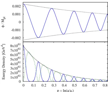
of φ at the peak of each oscillation is φmax = φia−1. Both of these behaviors can be seen in Figure 1, which shows the value of ϕ in the top panel and the kinetic and potential energy of the field in the bottom panel plotted over the course of several oscillations. These plots are generated from the numerical solution to Eq. (10) assuming ϕ′
i = 0 and ϕi = φi/MPl with β = 0.1 and κ= 2.
The fact that the quartic chameleon begins at φi≪MPl and does not exceed this value is an
interest-ing difference compared to runaway models. The field
-0.002 -0.001 0 0.001 0.002
φ
/ M
pl
0 1x1061 2x1061 3x1061 4x1061 5x1061 6x1061 7x1061 8x1061
0 0.1 0.2 0.3 0.4 0.5 0.6 0.7 0.8
Energy Density [GeV
4 ]
p = ln(a/ai)
FIG. 1: Top: The value ofϕ(blue, solid) and the values of its minima and maxima,−ϕia−1 andϕia−1, respectively (black,
dotted) over the course of four oscillations. Bottom: The kinetic (green, dashed) and potential (blue, solid) energies of the chameleon and their amplitude, Via−4 (black, dotted).
The potential energy reaches a maximum twice during each complete oscillation when|ϕ|is at a maximum. The kinetic energy reaches its maxima both timesϕpasses throughϕmin. At all times the chameleon energy density is much less than that of the radiationρ∗R∼(TJ,ia−1)4= 1064a−4GeV (In this
and all figuresβ= 0.1 andκ= 2.)
value at which runaway models become stuck due to fric-tion can be nearly equal toMPl[24]. If the field remains
stuck at such values until BBN, the large variation ofφ from its potential minimum can be interpreted as a larger variation in particle masses than we know to be allowed. Quartic chameleons, however, are already at field values much less thanMPl before the end of inflation and
os-cillate with a decreasing amplitude. While we will show that the field still finds its minimum prior to the kicks, it is not strictly necessary to avoid endangering the success of BBN.
Equation (8) implies thatφmin is proportional to the
cube root of the energy density in radiation and so will decay as a−4/3. Thus, φ
min will decrease faster than
the oscillation amplitude by a factor ofa−1/3, implying
the quantum effects associated with rapid changes in the chameleon field can significantly alter this classical be-havior.
III. QUANTUM CHAMELEONS
In chameleon models with runaway potentials, the only instances of rapid changes of the chameleon field after in-flation occur when the chameleon is kicked toward its po-tential minimum with a very high velocity and rebounds off its steep bare potential. The rapid changes in the mass of the chameleon during this rebound excite high-energy perturbations that, in a naive, classical evaluation, ex-ceed the energy initially available to the chameleon field. Considerations of the backreaction of particle produc-tion on the field showed that quantum correcproduc-tions signif-icantly alter the form of the potential experienced by the chameleon field. These corrections radically change the chameleon’s evolution throughout the rebound, causing it to turn around long before it would have exhausted the kinetic energy it possessed going into the rebound, which keeps the occupation numbers of the excited modes ex-tremely small [21].
In this section we show that every oscillation of the quartic chameleon excites perturbations, but with small enough energies that the energy lost to particle produc-tion does not exceed the initial energy of the field. For increasing values ofκwe find that the limit at which this is no longer the case coincides with the results Ref. [26], which also used quantum corrections to place an upper bound onκ. For the relatively large values ofκnear this limit, the field can lose all of its initial energy to particles before it completes an oscillation, and it simply falls to its potential minimum. For smaller values (κ .O(1)), the energy lost is only a small fraction of the field’s en-ergy at the start of an oscillation, and the evolution of the field over a single oscillation is not significantly al-tered. Instead, this energy loss accumulates over many oscillations and introduces an additional decay factor to the oscillation amplitude causing it to decay faster and reach its potential minimum.
A. Particle Production
We first summarize how rapid changes in the chameleon’s effective mass excite perturbations [29]; for a more detailed review of this process, see Appendix C of Ref. [21]. We begin by decomposing the field into its spatial average ¯φ(t) and the perturbationδφ:
φ(t,x) = ¯φ(t) +δφ(t,x). (17)
The linearized perturbation equation that governs the evolution ofδφis
∂t2+ 3H∂t−∇
2
a2 +V ′′ eff( ¯φ)
δφ= 0. (18)
Throughout this section we will not be using the vari-ablep, and primes will denote differentiation with respect to the argument of the function.
To quantize the perturbations, we introduce the cre-ation and annihilcre-ation operators ˆa†kand ˆak, respectively,
which obey the standard commutation relations,
h
ˆ ak,ˆa†k′
i
= (2π)3δ(3)(k−k′). (19)
The annihilation operator annihilates the vacuum state: ˆ
ak|0i= 0. Using ˆak† and ˆak we can then expressδφ(τ) as
ˆ
δφ(τ,x) =
Z d3k
(2π)3
ˆ ak
φk(τ)
a(τ) e
ik·x+ ˆa† k
φ∗
k(τ)
a(τ)e
−ik·x
,
(20) whereτ is conformal time. Inserting this decomposition ofδφ into Eq. (18), we find
φ′′
k(τ) +ω2k(τ)φk = 0; (21)
ωk2(τ) =k2+a2Veff′′( ¯φ)− a′′(τ)
a , (22)
whereω2
k(τ) is the effective mass of a plane-wave pertur-bation in the chameleon field with a comoving wavenum-berk.
During radiation domination a′′(τ) = 0, and
ω2k=k2+a2∗Veff′′ φ¯
≃k2+κ 2(a∗φ)
2, (23)
where in the last equality we have dropped the bar over φ as we will be working exclusively with the spatially averaged field. We also neglect the matter coupling be-cause it is subdominant to the bare potential throughout most of the oscillation. Whenω′
k(τ)/ω2k & 1, perturba-tions in the field are excited. Taking the derivative of this effective mass with respect toτ, we find
ω′
k(τ) =
a3 ∗
2ωk
h
2H∗V′′(φ) +V′′′(φ) ˙φ
i
;
= a
3 ∗
2ωk
h
κH∗φ2+κφφ˙
i
. (24)
We can simplify the last line of the equation by noting that not only is H∗φ2 initially smaller than φφ˙, it also
redshifts away faster. This can be seen by recalling the relations φmax = φia−1, ˙φmax = √2Kmax = √2Via−4, and using the fact that, during radiation domination,H∗
decreases asa−2. With these results, the maximum value
of the first term during each oscillation is H∗φ2max ≃ H∗,iφ2ia−4. The second term, however, is a product of two oscillating functions that reach their maxima at dif-ferent times. From the approximately sinusoidal nature of φ, we can determine that the product of φ and its derivative ˙φ will behave as the product of their ampli-tudes and another sinusoidal function, thus, (φφ˙)max is
proportional toφmaxφ˙max. The constant of
(φφ˙)max ∼φmaxφ˙max ≃ φia−1√2Kmax ≃pκ/12φ3ia−3. We can see thatH∗φ2∝a−4will decay away faster than φφ˙ ∝a−3. Thus, if H
∗φ2 is initially the smaller of the
two terms, we can neglect it. During radiation domination,H2
∗ ≃ρ∗R/(3MPl2), and
from Eq. (8), we know that φi = [24βρ∗R,i/(κMPl)]1/3.
Assuming that Ti = 1016 GeV, the relative contribu-tion between the two terms is p
12/κH∗,i/(0.6φi) ≃ 0.05(κβ2)−1/6. Thus, as long as κβ2 > 1.56×10⁻⁸,
which is true provided that neither β norκis unreason-ably small, this ratio is less than 1 and we can neglect theH∗φ2 term in Eq. (24).
By setting the ratio ω′
k(τ)/ω2k equal to 1, we can find the physical wavenumbers, kphys = k/a∗, of the
pertur-bations that are excited during the oscillations. Using Eqs. (23) and (24), we now have
ω′
k(τ)
ω2
k(τ)
≃ a 3 ∗
2ω3
k
κφφ˙,
=a
3 ∗
2
κφφ˙
k2+κ
2(a∗φ)2
3/2,
= κφφ˙
2hk2
phys+κ2φ2
i3/2. (25)
Setting this ratio equal to 1, and solving the last line for kphys, we get
k2phys=
κ
2φφ˙
2/3
−κ2φ2. (26)
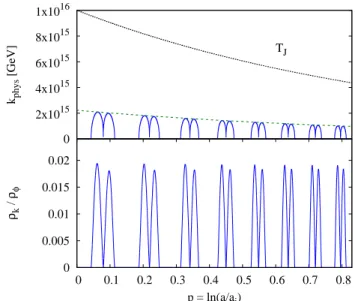
This expression reaches its maximum value four times during a single oscillation, as shown in Figure 2.
To evaluate kphys we again use how the maxima of
the contributing quantities are related to the initial field value and corresponding initial potential energy. Already we have established that, for the first term, (φφ˙)max = Aφmaxφ˙max, whereA≃0.6. It is also important to note
that the terms in Eq. (26) do not reach their maxima at the same timekphys is at its maxima. To account for
these proportionalities we introduce the numerical pa-rametersBandCto relate the maxima of the two terms to their values whenkphys is at its maxima. The
maxi-mum value ofkphys during an oscillation is then
kmaxphys
2
=Bκ
2Aφmaxφ˙max
2/3
−Cκ 2φ
2 max
=A2/3B
κ 2φia
−1
r
κ 12φ
4
ia−4
2/3
−Cκ 2φ
2
ia−2
= κ 2
"
A2
6
1/3
B−C
#
φ2
ia−2
kphysmax =D
r
κ 2φia
−1 (27)
=D(6κ)1/4Vi1/4a−1. (28)
0 2x10¹⁵ 4x10¹⁵ 6x10¹⁵ 8x10¹⁵ 1x10¹⁶
TJ
kphys
[GeV]
0 0.005 0.01 0.015 0.02
0 0.1 0.2 0.3 0.4 0.5 0.6 0.7 0.8
ρk
/
ρφ
p = ln(a/ai)
FIG. 2: Top: The value ofkphys (blue, solid) over four os-cillations. During each oscillation,kphys reaches a maximum four separate times at approximately the middle of the climb and decent on each side of the potential. The value of this maximum,kmax
phys (green, dashed), is on the order of the tem-perature and decays asa−1. Bottom: The ratio of the energy in the perturbations to the energy in the chameleon field over four oscillations. Each oscillation sees approximately a total 0.08 fractional loss of energy.
Forβ = 0.1 and κ = 2, B ≃ 0.6, C ≃ 0.1, and as it is defined in the last equation,D ≃0.4. Changing β orκ by two orders of magnitude does not significantly effect the value ofA,B,C, orD.
As well as being proportional to the oscillation am-plitude, the a−1 behavior of kmax
phys implies that it also
scales with the temperature. Starting from Eq. (27), the relationship betweenkmax
physand the Jordan-frame
temper-ature becomes apparent whenφiis determined by evalu-ating Eq. (8) using Σ = 4 andρ∗,i= (π2/30)g∗(TJ,i)TJ,i4 . After combining all numerical factors, we find that
kmaxphys≃2.67(κβ2)1/6
(T
J,i)4
MPl
1/3
a−1,
≃2.67(κβ2)1/6
T
J,i
MPl
1/3
TJ, (29)
where we have used the factTJ ∝a−1 during radiation domination.4 ForT
J,i = 1016GeV, β = 0.1, and κ= 2, the ratio ofkphysto the temperature iskphysmax/TJ ≃0.23, as shown in Figure 2.
The fact that the energy of the modes excited in quar-tic models is dependent only on the initial value of the field is another important contrast to runaway models. The energy of excited modes in such models is dependent on the velocity with which the chameleon approaches the minimum, ˙φM, which is of order GeV2. Reference [21] found that for a power-law potential of the form
V(φ) =Mv4
1 +
Ms
φ
n
, (30)
the most energetic mode that is excited has a physical wave number
kphys=
(n+ 2) 2√2
|φ˙M|
Ms
M
s ¯ φta
. (31)
where ¯φta.Msis the value ofφat which the field turns around. SinceMs∼meV, the ratio of ˙φM ∼TJ2andMs results in the excitation of extremely energetic modes even at low temperatures: kphys≫
q
˙
φM ∼TJ. For the quartic chameleon, however, highly energetic modes are only excited at high temperatures: kphys.TJ.
Using our value of kphys, we can evaluate the energy
density in the perturbations:
ρk =k
3n
kωk 2π2a4 ≃
k3 phys
2π2
q
k2
phys+V′′(φ),
= k
3 phys
2π2
r
κ
2φφ˙
2/3
−κ2φ2+κ
2φ
2,
= k
3 phys
2π2
κ
2|φφ˙|
1/3
, (32)
where nk ∼ 1 is the mode occupation number. In the same way that we foundkmax
physby relating the maxima of
the quantities in Eq. (26) to the initial potential energy, we can find the maximum ofρk during each oscillation,
ρmaxk =
D3
2π26 5/6κV
ia−4. (33)
From Section II we know that the chameleon’s energy density equals Via−4. Therefore, the maximum of the ratio ofρk and the energy at the start of an oscillation
ρφ is constant, as we can see in the bottom panel of Figure 2. The ratio of these two quantities is dependent onκ: ρk/ρφ≃0.01κ. To ensure our quantum corrections are kept under control, this ratio must be < 1, and we must have κ . 100. This is the same bound found by Ref. [26], which used another approach to limit quantum corrections. Runaway models could only keep this ratio less than 1 if the occupation number was extremely small, nk ≪1, which required altering the classical evolution of the field.
For κ&O(10) the chameleon field will lose all of its energy before it has a chance to complete its first oscilla-tion, at which point it will settle into its potential mini-mum. For smaller values ofκ, however, the depreciation
in the field’s energy is not as dramatic, and the small fractional loss of energy does not significantly affect the field’s evolution during a single oscillation. Instead, the effect accumulates over many oscillations, as we explore in the next section.
B. Effects of Particle Production forκ.O(1)
While the fraction of the energy lost in each oscillation is constant, the length of each oscillation period, ∆p, is not, as can be seen in Figure 2. The duration of the oscillations scales as follows:
∆p≃ 4ϕϕmax′ (p) avg
,
≃ 4ϕie −p
ϕ′ avg
, (34)
whereϕ′
avg is the average value ofϕ′ over a single
oscil-lation and once again primes denote differentiation with respect top. To more clearly see the behavior of ∆p, we first remark on the quantityϕ′ = ˙φ/(M
PlH∗). Radiation
domination implies thatH∗will decrease asa−2, and the
fact that the maximum kinetic energy of the chameleon during an oscillation, ˙φ2max/2, is proportional to a−4
im-plies that ˙φmaxalso decreases asa−2. Therefore, the
am-plitude of the ϕ′ oscillations is a constant value: ϕ′ max.
Sinceϕ′
max is constant, so too is its average, and ∆p
de-cays with the amplitude ofϕ. The two valuesϕ′ avg and ϕ′
max can be related by a constant scaling factor found
numerically to be q ≡ϕ′
avg/ϕ′max ≃0.76, and is highly
insensitive to changes in β and κ of up to 2 orders of magnitude.
When considering the energy lost during each oscil-lation, it is useful to consider how the quantities ϕmax
and ϕ′
avg are related to the energy at the start of each
oscillation,ρ(p):
ϕmax(p) =
4!
κ ρ(p) M4
Pl
1/4
(35)
ϕ′
max(p) =
˙ φmax H∗MPl
=
p
2ρ(p) H∗MPl
=
r
κ 12
MPl H∗
ϕ2max(p),
(36)
where we have used the fact that the maximum kinetic energy that occurs during each oscillation, ˙φ2
max/2, is
equal to the potential energy at the start of each oscilla-tion. Using Eqs. (35) and (36) and the scaling constant q, Eq. (34) then becomes
∆p=4 q
r
12 κ
H∗ MPl
ϕ−1max,
=4 q
6
κ
1/4
Hie−2pρ−1/4, (37)
= 1 Qe
whereHiis the initial Hubble value at the end of inflation and in the last line we have condensed all the constants into one constant,Q−1.
Over the course of each oscillation, the energy of the chameleon field decreases by a factor of e−4∆p due the expansion of the Universe, as well as by an additional factor due to the creation of particles. If we takef .1 as the fraction of energy left after the field has lost energy due to the production of particles during one oscillation, we can write the change in energy over one oscillation period as
∆ρ ∆p =
f ρinite−4∆p−ρinit
∆p ,
≃f ρinit(1−∆4∆pp)−ρinit. (39)
Iff= 1 we recover the originalρ∝e−4pevolution. Using Eqs. (38) and (39) we can write a differential equation for the energy loss including particle production,
dρ dp =−ρ
1−f ∆p + 4f
=−Q(1−f)e2pρ5/4−4f ρ (40)
The second term in Eq. (40) gives the classical ρ∝a−4
evolution and dominates at smallp. But thee2pfactor in the first term allows it to quickly dominate over the sec-ond term. If we consider the regime in which the secsec-ond term has become negligible, we can integrate Eq. (40) and see that the energy will follow an entirely different behavior at late times:
dρ
dp =−Q(1−f)e 2pρ5/4
Z dρ
ρ5/4 =−Q(1−f)
Z
e2pdp
ρ=
Q(1
−f)
8 e
2p+C
−4
(41)
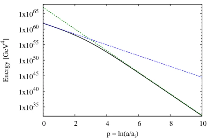
where C is a constant of integration. At large values ofp, when this behavior is relevant, the exponential term will dominate over the constant and the energy will scale as e−8p. The two regimes and behavior of ρcan be seen in Figure 3. Thepvalue at which thee−8p behavior begins to take over is determined byκ, with larger values ofκ leading to an earlier change in regimes.
When the e−8p term begins to dominate, the ampli-tude of the oscillations will then decay as e−2p. This is faster than its original e−p behavior and, more im-portantly, faster than thee−4p/3 decay of the minimum
of its effective potential. The oscillation amplitude will then decrease below the value ofφmin and the field will
fall into its minimum.
We have seen that the oscillatory motion of the chameleon in a quartic well creates large variations in the field’s mass. Particle production must be considered, but the inclusion of these quantum effects does not result in
the catastrophic effects experienced by other chameleon potentials. Instead the energy of excited modes is com-parable to the temperature and the fraction of the initial energy lost to particle production is always less than 1 as long asκ.100. Next we investigate whether quartic chameleons can also avoid the problems runaway models encounter when facing the kicks.
IV. KICKING THE QUARTIC CHAMELEON
After the depletion of energy to particle production takes the chameleon field to or near the minimum of its effective potential, we can show that it will track its minimum until the onset of the kicks. The characteristic time scale for the evolution of the minimum isφmin/φ˙min,
whereas the characteristic time scale of the response of the field is given bym−1. When the field is in the
mini-mum of its effective potential,
m2= d2V dφ2
φ=φmin
= κ 2φ
2 min=
9
2κ
1/3βΣ
MPl ρ∗
2/3
.
(42) If m ≫ φ˙min/φmin, the field will adiabatically track its
minimum. To compare these values, first we must deter-mine ˙φmin:
˙
φmin=H dφmin
dp ,
= 2β κMPl
H φ2
min
ρ∗RdΣ
dT + Σ dρ∗R
dT
dT dp,
≃κM2β Pl
H φ2
min ρ∗R
dΣ
dT + 4 Σ T
(−T),
=−13Hφmin
4 +T Σ
dΣ dT
, (43)
where we have used the definition of φmin given by
Eq. (8), the fact thatρ∗∝T4∝a−4, and thatφ≪MPl
implies T ≃ TJ. If Σ is constant, the second term in parentheses drops out, and we recover theφmin∝a−4/3
behavior we determined in Section II. Thus, when Σ is constant, the evolution of the minimum is set by the ex-pansion rate, and the characteristic time scale is approx-imately the Hubble time H−1. Comparing this to the
mass of the field in its minimum, we have
m2
˙
φmin φmin
2 =
4 3
m2 H2 =
4 3
9 2κ
1/3
βΣ MPl
ρ∗
2/3
3M2 Pl ρ∗
,
= 4
9
2κβ
2
1/3 Σ2M4
Pl
π2
30g∗T4
!1/3
. (44)
We can see that, for reasonable values ofκ and β, the mass of the field at its potential minimum is much greater thanH for allT ≪MPl while Σ is constant.
1x1035 1x1040 1x1045 1x1050 1x1055 1x1060 1x1065
0 2 4 6 8 10
Energy [GeV
4 ]
p = ln(a/ai)
FIG. 3: The energy in the chameleon field at the peak of each oscillation (black, solid), showing the effect of particle production on the energy decay, found by numerically solving Eq. (40). While the energy begins redshifting asa−4 (blue, dotted), particle production eventually dominates the energy loss and the energy decays asa−8 (green, dashed).
thanH. However, even in this region, the constant na-ture of Σ due to the QCD trace anomaly does not allow the field to become stuck due to Hubble friction. In this small region the effective potential is dominated by the matter coupling; if we neglect the driving term from the bare potential and use the fact that V ≪ ρ∗R, we can simplify Eq. (10) to
ϕ′′=−ϕ′−3βΣ. (45)
Integrating this equation for a chameleon initially at rest gives
ϕ′≃3Σβ 1−e−p
. (46)
From this we see thatϕ′ will increase toward a constant
value until the field approaches its potential minimum and the bare potential can no longer be neglected. Thus, even if the chameleon begins at rest in a region where it has a low effective mass, Hubble friction will not prevent it from reaching its potential minimum. We have just shown in Eq. (44) that once it reaches this minimum it will then track it adiabatically.
Having established that the chameleon oscillates about its minimum at the onset of the kicks, we can now look at how they will affect the field’s evolution. Comparing mand ˙φmin/φminwhen Σ is no longer constant, we have
m2
˙
φmin φmin
2 =
m2 H2
9
4 + TΣddTΣ2.
(47)
The kick function Σ displays two different types of be-havior: at the beginning of the kicks when the tempera-ture is greater than the mass of the particle species,mi,
Σ∝m2
i/T2, and at the end of the kicks, when T < mi, Boltzmann suppression makes Σ∝e−mi/T. We can
esti-mate the ratio in Eq. (47) using these two behaviors and the ratiom2/H2 given by Eq. (44). At the beginning of
the kicks, whendΣ/dT =−2Σ/T,
m2
˙
φmin φmin
2 =
m2 H2
9 4
≃
ΣM2
Pl T2
2/3
. (48)
Even though Σ≪1, the quantity (MPl/T)2is more than
sufficient to make this ratio≫1. At the end of the kicks, however, whendΣ/dT =−miΣ/T2,
m2
˙
φmin φmin
2 =
m2 H2
9 4 + mi
T
2
≃
ΣT M2
Pl m3
i
1/3
, (49)
which is only>1 as long asM2
Pl/m3i >(ΣT)−1. This is true up until the end of the electron-positron kick, when the temperature and the value of Σ continue to decrease past the point thatM2
Pl/m3ecan no longer compensate for their increasingly small values. Forβ = 0.1 and κ= 2, this occurs at approximately a temperature of 39 keV, whenφmin∼10−33MPl.
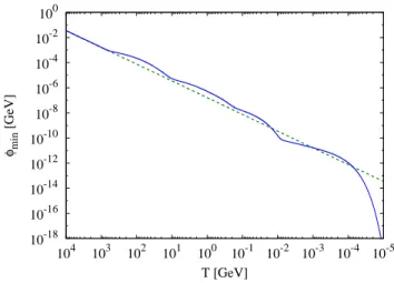
Figure 4 shows the value ofφmin as a function of the
temperature. The solid line shows the minimum under the influence of the kicks, while the dashed line shows the minimum following thea−4/3 decay when Σ is
con-stant. The effect of the kicks for the most part is to slow the decrease in the minimum of the effective po-tential compared to this decay, until the very end of the kicks when Boltzmann suppression drastically decreases the value of Σ. In Figure 5 we have plotted the exact value of the ratio in Eq. (47), and we can see that the ra-tio is indeed much greater than 1 until after the last kick. Therefore the chameleon will track its minimum adiabat-ically until then. When this occurs, even if we assume the field becomes entirely stuck while the potential mini-mum continues to decrease toward zero, the deviation of the field from its minimum cannot exceed the value at which it was stuck: ∼10−33M
Pl. This is clearly≪MPl
and any implied variation in the particle masses would be completely negligible. When the Universe later becomes matter dominated and Σ = 1, the field will once again be able to track the minimum of its effective potential.
V. CONCLUSION
10-18 10-16 10-14 10-12 10-10 10-8 10-6 10-4 10-2 100
10-5 10-4 10-3 10-2 10-1 100 101 102 103 104
φmin
[GeV]
T [GeV]
FIG. 4: The value ofφmin during the kicks (blue, solid) and the extrapolation of the e−4p/3 behavior experienced during the period when Σ is constant (green, dashed). The value of φminduring the kicks actually decreases at a slower rate than it did when Σ was constant until the end of the last kick.
of the Universe without the addition of a constant term to its potential [3], the field’s sensitive dependence on its en-vironment gives it remarkable properties that are of great interest. However, for most chameleon models, the same matter coupling that gives it its unique phenomenology leads these theories into trouble in the early Universe. The meV mass scale of runaway potentials is at odds with the GeV mass scale of SM particles, which acceler-ate the chameleon field to very high velocities when they become nonrelativistic. The hierarchy between these two energy scales leads to the quantum production of parti-cles that radically alters the field’s evolution. Without very weak couplings or highly tuned initial conditions these chameleon models cannot be trusted as effective field theories at the time of BBN [20, 21].
In this paper, we have considered the quartic chameleon potential, which is not often studied in the-ories of chameleon gravity. A significant feature of this model is the fact that there is no mass scale in the poten-tial: the chameleon’s self-interaction is enough to ensure adequate screening. We have shown that this scale-free property of the potential allows the quartic chameleon to avoid the catastrophic effects of the small energy scales within runaway models.
After inflation, the quartic chameleon oscillates in its potential well. The amplitude of its oscillations are damped due to Hubble friction. In the classical treat-ment, the minimum of the field’s effective potential de-creases faster than the oscillation amplitude throughout radiation domination. Consequently, the field cannot reach its potential minimum before BBN, though the os-cillation amplitude is always sufficiently small that the variation of the field from this minimum does not imply an unacceptable variation from known particle masses.
The rapid oscillations of the chameleon field cause changes in its effective mass that excite perturbations
10-5 100 105 1010 1015
10-5 10-4 10-3 10-2 10-1 100 101 102 103 104
m
2 / (
φ
. min
/
φmin
)
2
T [GeV]
FIG. 5: The numerical evaluation of the ratio in Eq. (47), which is significantly greater than 1 throughout the kicks. It becomes less than 1 whenT ≃3.9×10⁻⁴GeV.
and lead to particle production. The effects of quantum particle production ensure that the field does reach its potential minimum while the Universe is radiation domi-nated. For large values (&10) of the self-interaction con-stantκ, the fractional loss of energy to these particles can be large, in which case the field loses all its energy in the course of a single oscillation. For smallerκ, the energy lost to particles constitutes only a small fraction of the field’s energy. This much slower energy loss accumulates over multiple oscillations and introduces an additional decay term to the oscillation amplitude which allows the field to catch its minimum after many oscillations. At this point, the field will adiabatically track its potential minimum. It will track this minimum until the very tail end of the kicks, when the Boltzmann suppression of Σ decreases the value ofφmin faster than the field can
fol-low. The value of the field at this point is sufficiently small that any deviation of particle masses implied by the deviation of the field from its potential minimum are entirely negligible.
Acknowledgments
We thank Kayla Redmond for her comments on our manuscript. C.M. acknowledges support from the Bahn-son Fund at the University of North Carolina at Chapel Hill.
Appendix: Energy Densities in Chameleon Gravity
In this appendix we take a closer look at the energy evolution of different quantities in the Jordan and Ein-stein frames.
1. Energy Density of Matter and Radiation
In order to consider the quantities that are conserved in both the Einstein and Jordan frames recall how the energy density and scale factor in each frame are related, namely, ˜ρ = e4βϕρ
∗ and ˜a = e−βϕa∗, where we have
used the dimensionless variable ϕ = φ/MPl . Matter
and the chameleon field do not interact in the Jordan frame and so the matter stress-energy tensor is conserved,
˜
∇µT˜µν = 0, and we can write the conservation equation in the Jordan frame,
˜
ρ∝˜a−3(w+1). (50)
Exchanging the Jordan frame quantities for those of the Einstein frame, we have
ρ∗e4βϕ∝ a∗e−βϕ
−3(w+1)
,
ρ∗e4βϕ∝a∗−3(w+1)e3βϕ(w+1),
ρ∗eβϕ(1−3w)∝a−3(∗ w+1). (51)
For matter we havew= 0 and Eq. (51) becomes
ρ∗meβϕ∝a−3∗ . (52)
Clearly, the Einstein-frame energy density in matter, ρ∗m, does not scale as a−3∗ . This follows from our
ear-lier statement in Section II that the stress-energy ten-sor that is conserved in the Einstein frame is not T∗µν, but the sum of T∗µν and the stress-energy tensor of the chameleon field. Often it has been the practice to define the left-hand side Eq. (52) as the matter density as it is the quantity that follows the conservation equation in the Einstein frame [2, 24].
For radiation, however, w = 1/3 and we find from Eq. (51) that
ρ∗R∝a−4∗ . (53)
In both frames the energy density in radiation is propor-tional toa−4
∗ , and it follows thatH∗ ∝a−2∗ .
2. Energy Density of the Chameleon
In Section II we used the canonical definitions of the energy density and pressure of a scalar field, namely ρφ= ˙φ2/2 +V and Pφ = ˙φ2/2−V, to determine its equation of state, w. However, when defining w in this way, because the field’s coupling to matter allows it to exchange energy with the matter fields, the chameleon does not follow the conservation equation,
˙ ρφ
ρφ −
3H∗2(1 +w)6= 0. (54)
If we instead introduce a new pressure,
Pn= 1 2φ˙
2
−V −3H1 ∗
˙ φ β
MPl
Σρ∗ (55)
we can see that with this new definition, the field now obeys the conservation equation,
˙
ρφ+ 3H∗(ρφ+Pn) =
= ˙φφ¨+dV
dφφ˙+ 3H∗ ˙ φ2
2 +V + ˙ φ2
2 −V − 1 3H∗
˙ φ β
MPlΣρ∗
!
= ˙φ
¨
φ+ 3H∗φ˙+ dV dφ −
β MPl
Σρ∗
. (56)
The terms in parentheses in the last line make up the chameleon’s equation of motion, Eq. (5), and the entire quantity in parentheses is indeed equal to 0. While we used the canonical form of the pressure in the text, we also took its average value over many oscillations, and the term which we have added to the potential is not positive-definite, and will average to 0.
Not only will it average to 0, but we can also show that the additional contribution to the new pressure is negli-gible compared to the usual terms. Using the relation
˙
φ=H∗MPlϕ′, we can rewrite Pn as
Pn = 1
2(H∗MPlϕ
′)2
−V −13ϕ′βΣρ∗
=1 6ρ∗ϕ
′2
−V −13ϕ′βΣρ∗. (57)
The maximum values of the first two terms, the kinetic and potential energies of the field, are equal and so to compare the relative contribution of the last term, we will look specifically at how it compares the kinetic energy. The maximum value reached by ϕ′, given in Eq. (36),
can be broken down further using the initial values of the field andH∗,
ϕ′max=
r
κ 12
s
3 ρ∗,i
6βΣiρ∗,i
κMPl
2/3
≃
β4
κ
1/681
4 Σ
4
i
ρ∗R,i
M4 Pl
1/6
Combining numerical factors and usingTJ,i= 1016GeV we have
ϕ′
max= 0.19
β4
κ
1/6
. (59)
The relative contribution of the two terms is then
βΣ/ϕ′
max ∼ 0.005(κβ2)1/6, which for even some of the
larger values of κ and β allowed (κ = 100, β = 1) is still much less than 1. Therefore, the additional term is a negligible contribution to the canonical pressure, and our use of the conservation equation, Eq. (16), is valid.
[1] J. Khoury and A. Weltman, Phys. Rev. Lett.93, 171104 (2004), astro-ph/0309300.
[2] J. Khoury and A. Weltman, Phys. Rev. D69, 044026 (2004), astro-ph/0309411.
[3] J. Wang, L. Hui, and J. Khoury, Phys. Rev. Lett.109, 241301 (2012), 1208.4612.
[4] P. Hamilton, M. Jaffe, P. Haslinger, Q. Simmons, H. M¨uller, and J. Khoury, Science 349, 849 (2015), 1502.03888.
[5] K. Li et al., Phys. Rev.D93, 062001 (2016), 1601.06897. [6] H. Lemmel, P. Brax, A. N. Ivanov, T. Jenke, G. Pignol, M. Pitschmann, T. Potocar, M. Wellenzohn, M. Zawisky, and H. Abele, Phys. Lett.B743, 310 (2015), 1502.06023. [7] A. D. Rider, D. C. Moore, C. P. Blakemore, M. Louis, M. Lu, and G. Gratta, Phys. Rev. Lett. 117, 101101 (2016), 1604.04908.
[8] A. Almasi, P. Brax, D. Iannuzzi, and R. I. P. Sedmik, Phys. Rev.D91, 102002 (2015), 1505.01763.
[9] C. Burrage, E. J. Copeland, and J. A. Stevenson, JCAP
1608, 070 (2016), 1604.00342.
[10] G. Rybka, M. Hotz, L. J. Rosenberg, S. J. Asztalos, G. Carosi, C. Hagmann, D. Kinion, K. van Bibber, J. Hoskins, C. Martin, et al., Physical Review Letters
105, 051801 (2010), 1004.5160.
[11] J. H. Steffen, A. Upadhye, A. Baumbaugh, A. S. Chou, P. O. Mazur, R. Tomlin, A. Weltman, and W. Wester (GammeV), Phys. Rev. Lett. 105, 261803 (2010), 1010.0988.
[12] V. Anastassopoulos et al. (CAST), Phys. Lett. B749, 172 (2015), 1503.04561.
[13] G. Cantatore, A. Gardikiotis, D. H. H. Hoffmann, M. Karuza, Y. K. Semertzidis, and K. Zioutas, in Proceedings, 11th Patras Workshop on Axions, WIMPs and WISPs (Axion-WIMP 2015): Zaragoza, Spain, June 22-26, 2015 (2015), 1510.06312, URL
https://inspirehep.net/record/1399180/files/arXiv:1510.06312.pdf. [14] S. Baum, G. Cantatore, D. H. H. Hoffmann, M. Karuza,
Y. K. Semertzidis, A. Upadhye, and K. Zioutas, Phys.
Lett.B739, 167 (2014), 1409.3852.
[15] B. Jain, V. Vikram, and J. Sakstein, Astrophys. J.779, 39 (2013), 1204.6044.
[16] H. Wilcox et al., Mon. Not. Roy. Astron. Soc.452, 1171 (2015), 1504.03937.
[17] H. Wilcox, R. C. Nichol, G.-b. Zhao, D. Bacon, K. Koyama, and A. K. Romer (2016), 1603.05911. [18] P. Brax, C. van de Bruck, S. Clesse, A.-C. Davis,
and G. Sculthorpe, Phys. Rev. D89, 123507 (2014), 1312.3361.
[19] D. Boriero, S. Das, and Y. Y. Y. Wong, JCAP1507, 033 (2015), 1505.03154.
[20] A. L. Erickcek, N. Barnaby, C. Burrage, and Z. Huang, Phys. Rev. Lett.110, 171101 (2013), 1304.0009. [21] A. L. Erickcek, N. Barnaby, C. Burrage, and Z. Huang,
Phys. Rev.D89, 084074 (2014), 1310.5149.
[22] S. S. Gubser and J. Khoury, Phys. Rev. D70, 104001 (2004), hep-ph/0405231.
[23] A. Padilla, E. Platts, D. Stefanyszyn, A. Walters, A. Weltman, and T. Wilson, JCAP 1603, 058 (2016), 1511.05761.
[24] P. Brax, C. van de Bruck, A.-C. Davis, J. Khoury, and A. Weltman, Phys. Rev. D70, 123518 (2004), astro-ph/0408415.
[25] D. F. Mota and C. A. O. Schelpe, Phys. Rev. D86, 123002 (2012), 1108.0892.
[26] A. Upadhye, W. Hu, and J. Khoury, Phys. Rev. Lett.
109, 041301 (2012), 1204.3906.
[27] E. G. Adelberger, B. R. Heckel, S. A. Hoedl, C. D. Hoyle, D. J. Kapner, and A. Upadhye, Phys. Rev. Lett. 98, 131104 (2007), hep-ph/0611223.
[28] R. R. Caldwell and S. S. Gubser, Phys. Rev.D87, 063523 (2013), 1302.1201.