of Infrastructure Service Contracts
by Thomas E. Wendling
ABSTRACT
A firm will replace a physical asset at the end of its useful life. This fact
dem-onstrates that there is a notion of mortality implicit in the way an enterprise
manages its physical assets. We propose a theory that there is also an
effi-cient time to replace a physical asset that is random and observable.
Sepa-rate economic and financial models converge on agreement that (1) there is
only one instant in time that an asset must be replaced in order to minimize
the present value cost impact to the enterprise; (2) that this efficient instant
is observable, and a function of both the enterprise’s cost of capital and
readily obtainable current calendar year information; and (3) that the time
to this efficient instant is random, and may be infinite. Through a policy of
coordinating the timing of replacements with these efficient, observable
instants, lost efficiencies are recovered. Such a policy necessarily creates
volatile, fortuitous, future cash flows, which are dealt with through capital
adequacy or risk transfer, rather than deferral or other forms of scheduling
for convenience. The efficiency gains and accompanying value creation
may be material if the enterprise’s assets are mostly physical.
According to Evans and Annunziata (2012) a one-percent efficiency savings applied across these spe-cific global industry sectors could result in an addition of $15.3T to global GDP by 2030.
Matziorinis and Rowley (1993) describe the mag-nitude of physical asset expenditures and some of the shortcomings in the way they are accounted for on a macroeconomic level. They focus on repair and replacement expenditures only, and express the opin-ion that these do not receive much attentopin-ion in the theory and econometrics of investment, despite their importance. They also describe the effect of the level of aggregation of physical assets in the accounting of such expenditures as a reason they cannot be consis-tently measured. For example, is an airplane a single physical asset, or is it composed of the airframe, engines, and interior fittings as separate assets?
Work has been done attempting to explain the economic reasons for replacement investment. Eisner (1972), Feldstein and Foot (1971), and Feldstein (1974) have studied statistical correlations in empirical data classified into different candidate determinant vari-ables, including a firm’s liquidity, cost of capital, level of sales, level of expansion investment, level of capac-ity utilization, business expectations, rate of change in capital goods prices, the average age of capital goods, tax factors, and technology change. Interesting correla-tions among these variables were discovered by these authors, and subsequent works which cite them have used their findings to address the accuracy of macro-economic measures, such as gross fixed capital expen-diture or gross fixed capital formation. These authors also considered behavioral effects implicit in these explanatory variables, which we intend to filter out by articulating a purely rational enterprise policy for the replacement of physical assets.
2. Infrastructure service
contracts (ISCs)
In enterprise risk management, there is usually a lack of appropriate risk transfer mechanisms for opera-tional risks. In this paper, we will suggest the deliber-ate creation of volatile, risky cash flows resulting from
1. Introduction
This paper predicts the existence of potentially substantial economic inefficiencies borne by organi-zations that are not detectable through examination of data created by currently configured accounting systems. Its conclusions are predicated on assump-tions about the nature of a function called M(t), which defines the size and timing of opportunity costs unique to individual physical assets. Certain gross characteristics of M(t) will be described, and are simply assumed for the purpose of building a theoretical argument which could form the basis for an enterprise policy to manage physical assets.
The physical assets referred to in this paper are fixed assets that are not expended during operations, and are used to produce revenues. They do not include cash or inventories, which might sometimes be included under a broader definition. They comprise the plant, property, and equipment line item on the balance sheet. These assets are sometimes collectively referred to as plant. Many physical assets will eventually be replaced with like or similar assets that perform the same mis-sion within the plant. The process of replacing physical assets when they have reached the end of their useful lives is often referred to as renewal.
The value of physical assets in the economy is vast. Of particular interest in this paper is capital equipment. According to the United States Census Bureau (USCB 2012), $7.212T of capital equipment was purchased between 2001 to 2010 in the United States alone. Much of it will be replaced in the future when it becomes obsolete. Subsequent years will probably show increas-ing levels of investment in capital equipment.
We refer to the entities described above as ser-vice providers. They have a direct contractual rela-tionship with the facility owner to provide a wide range of services, including repair and replacement of capital assets. The facility owner is the contract holder, and is usually a utility, municipality, or trans-portation authority. Replacement of physical assets usually refers to the replacement of a whole item of capital equipment or a structure, such as machinery or a building.
Service providers are responsible for complete facility maintenance, including routine maintenance, repairs, and replacements of physical assets. The agreement to provide repair and replacement ser-vices is a part of a larger offering of serser-vices, and is now often set forth in distinct articles within such contracts. In the past, these obligations were infor-mally agreed to and not meticulously documented. Recently, as this infrastructure delivery method has gained traction in the United States, attorneys have attempted to formalize physical asset replacement obligations. Spelling out these obligations has forced negotiating parties to explicitly consider the eco-nomic aspects that the contract must capture for an equitable transfer of risk and fair pricing.
In this paper, only the long duration repair and replacement obligations under such contracts are referred to as infrastructure service contracts (ISCs). This definition, unique to this paper, allows us to sepa-rate and focus only on the services that are a very near counterpart to home and vehicle extended service contracts with which they share many similarities.
Manufacturers of capital equipment have also pro-vided extended service contracts covering repairs and replacements associated with their products. This is partly in response to the needs of service providers who wish to transfer these risks, and manufacturers’ willingness to assume such risks as a value added ser-vice in order to sell capital equipment. A manufac-turer will often provide an extended service contract which matches the duration and requirements of the service provider’s contract with facility owners.
As with their home and vehicle counterparts, the exposure to risk in ISCs varies significantly during asset replacements in order to achieve a higher level of
operational efficiency. Fortunately, there already exists an institution for transferring such risks. Extended service contracts can be used to implement physi-cal asset replacement policies. This section serves as an introduction to such contracts for facilities and infrastructure, and intends to provide some historical background on the environment in which the theory described in this paper was conceived.
As there are extended service contracts for homes and vehicles, so there are long duration repair and replacement agreements for whole industrial facili-ties and public infrastructure. Unlike their home and vehicle counterparts, such extended warranties for facilities and infrastructure do not exist as stand-alone products. Rather, they are underwritten in the limited context of non-insurance entities providing entire railways, water treatment plants, power plants, or other large ensembles of physical assets.
Contracts in which single entities provide integrated engineering, procurement, construction, operations, routine maintenance, repair and replacement services to deliver and run new facilities and infrastructure may have first come into existence in the 1980s, and possi-bly much earlier if one includes public-private partner-ships for public utility infrastructure which date back to the late nineteenth century. Companies specializing in one or more of the above services usually must form consortia to meet the wide scope of responsibilities required under such contracts. Contract terms can be as long as 50 years, and entities providing these ser-vices assume most of the functional roles of the owner of the facility.
Some contracts stipulate a required physical condi-tion of the facility at the end of the contract term. This can be specified as a threshold minimum weighted average useful life of covered facility capital equip-ment at the end of the contract term, in which esti-mated equipment replacement costs weight estimates of remaining useful equipment life, as determined by a facility condition assessment conducted by a third-party evaluator.
Some contracts use verbal thresholds to describe the minimum required physical condition of equipment and structures at the end of the term. If the facility does not meet these qualitative descriptions, then the service provider must make all repairs, replacements, or cash payments necessary to remedy the deficiencies.
The service provider usually cannot terminate the contract for convenience, nor modify the service fee during the term of the contract. The service fee can be automatically indexed for inflation. An indexing for-mula is usually a pre-negotiated part of the contract, not subject to modification after the contract is exe-cuted. Common indexes used are a weighted combi-nation of Consumer Price Index (CPI), Employment Cost Index (ECI), and other indexes published by the Bureau of Labor Statistics (BLS).
As with their automobile and home counterparts, ISCs are secondary to short-term warranties against defects in workmanship provided by the equipment manufacturer (original equipment manufacturer or OEM) or equipment seller. However, this is small comfort to the service provider who essentially pro-vides a warranty many times longer than the OEM warranty. OEM warranties for capital equipment can typically last 18 months from delivery or 12 months from time of use, whichever comes first. This period is small compared to the 10- to 50-year terms of ISCs.
Some contracts also include a negotiated list of major equipment subject to replacement obligations. Each item of equipment may have a cap for replace-ment cost reimbursereplace-ment to the service provider, but replacement obligations are limited to those items on the list.
ISCs usually do not have explicit service fees. Coverage is often bundled as a part of a larger ser-the contract period, and pro rata earning of service
fees does not provide a match between income and liabilities. In addition, service fees are not always received in proportion to the level of exposure to risk. Unlike their home and vehicle counterparts, earning patterns are not easily predicted by traditional prop-erty and casualty methods using data triangles. There is little historical loss data, and the tails for such coverage can be far longer than these contracts have been in existence.
The entities that underwrite ISCs are not insur-ance companies. To our knowledge, insurers are not involved in underwriting long duration repair and replacement risks associated with industrial and pub-lic infrastructure. There are several reasons for this, which will be discussed later. Facility owners trans-fer these risks to service providers. Then service providers transfer some of these risks to manufac-turers. In both of these transactions, the underwriting of repair and replacement losses is always only a por-tion of the total services rendered. Beyond the service provider and manufacturer, there is no further place to transfer this risk.
2.1. Typical features of the ISC
In an ISC, the service provider agrees to replace physical assets during the term of the contract. Because of the long term of these contracts, a large proportion of the covered capital equipment in a facility may be replaced, perhaps multiple times. Repairs are an important part of the scope of an ISC, but the major-ity of losses and expenses arise from the contract’s replacement obligations.
sity of pricing such contracts has resulted in several methods for forecasting future losses associated with these contracts. Under FAS 5, if the amount is not reasonably estimable, then no accrual of a liability is necessary. Since no standard actuarial method for estimating such unpaid liabilities exists, they might be deemed as not reasonably estimable.
The difficulty in projecting capital equipment repair and replacement losses stems from a lack of recorded historical experience. Owners of physical assets keep maintenance records, but they are incom-plete, without standard format, often proprietary, and have not been around for very long. There is no cen-tral repository for this data, nor are there vital statis-tics on the longevity of capital equipment. Contract conditions are extremely varied, and service providers have such sparse information individually that the usual actuarial methods would not be useful to pro-duce projections of loss emergence over the life of the contract.
Furthermore, since we are addressing the sub-ject of mortality, the actuarial nature of this analysis more closely resembles a life contingency problem for which an approach using customary data trian-gles may not be appropriate. Unlike death benefits, however, repair and replacement liabilities under ISCs are distant future property losses, and are infla-tion sensitive.
Central to estimating loss costs due to equipment replacements are estimates of equipment longevity. However, there are no life tables for the diverse types of capital equipment used in widely varying indus-tries. A gas turbine will not have the same expected lifespan as a dump truck, or even another gas turbine in a different industry. There are published account-ing guidelines on useful life of physical assets, but they follow very broad classifications, and are used mostly for depreciation purposes. There are also manufacturer’s claims of equipment longevity, but these may be biased. Even though these guidelines have some basis in reality, they are only point values with no information on the variance of asset lifespan.
The method employed to project losses and expenses must take into account the life contingency nature vice fee for ongoing operations and maintenance
services, which can include consumables, power, labor, and scheduled maintenance. Fees can be paid as a level monthly amount (subject only to index-ing as described above) over the contract term. Alternatively, some fee payment structures separate the ISC (repair and replacement) component from the total service fee, and try to match fee payment with the expected emergence of losses. The latter payment method implicitly recognizes that new infrastructure will probably not incur significant repair and replacement losses until decades after the beginning of the contract. The contract holder usually requests this, since ISCs normally do not have provisions for the refund of unearned services fees should the owner decide to cancel the contract prematurely.
ISCs also exist for older facilities in military utilities privatization. These contracts are riskier for service providers, since the condition of the facility is difficult to assess without a costly inspection that must be conducted prior to bidding on such services. Unlike service contracts for new facilities, these are usually underwritten only by companies provid-ing complete operations and maintenance services. Manufacturers will seldom underwrite unscheduled maintenance obligations on old capital equipment that has been in operation for a while.
Level service fees are usually charged throughout the life of the contract, indexed for inflation, but with no other modification. Because the fees associated with ISCs can be high (ranging from $100,000 per year for a small water treatment plant to $25,000,000 per year for a city light rail system), the considerable time and expense of underwriting, which involves item-by-item estimation of asset repair and replace-ment costs, is justified.
2.2. Projecting future losses of ISCs
neces-easy to purchase a water heater at the hardware store as an immediate alternative to an expensive repair. In contrast, in an industrial setting, it is not so easy, for example, to purchase a locomotive as an imme-diate alternative to repairing one. The procurement process from requisition to commissioning can last years. Even prior to such a requisition, the decision to replace a major item of capital equipment is the result of a lengthy process, which begins with the gradual (and often delayed) recognition of the eco-nomic benefits of replacement, and is often deferred due to management incentives and the lack of avail-ability of scarce funds for asset replacements.
Capital equipment seldom generates repair costs from a single mechanical failure close to the all-in replacement cost of the equipment. Therefore, the repair versus replacement rationale described at the beginning of the last paragraph may hold for home, vehicle, or appliance service contracts, but it has little application with capital equipment.
Repairs are triggered when equipment or com-ponents fail. Repairs cannot be deferred, since they are required to restore equipment to functionality, which can be critical from the standpoints of safety, reliability, availability, or lost revenues. However, replacement of a physical asset is deferrable, in favor of continued repairs, even though it may not always be economically efficient to do so.
And what of the role of technological obsolescence in a replacement decision? Obsolescence is the state of a fixed asset, service or process when it becomes unwanted or should no longer be used. However, the asset may still be useful (and usually is) in good working order. In industry, obsolescence is thought to occur because a like replacement is available that is economically superior in some way. A replacement asset may have comparative advantages to the exist-ing asset, such as savexist-ing time or reducexist-ing energy usage, potential costs of downtime, or consumption of scarce resources. Obsolescence may be due to the availability of new technology or the aging condition of the asset itself.
Few actions have as powerful an impact on the operating costs of an individual physical asset as of this problem, but must also work with the limited
amount of data available on equipment longevity. The method should not entrain superfluous assump-tions due to the absence of data. If an assumption must be made, then the results should be com-pared to those from other alternative assumptions. Wendling (2011) outlines a simulation method for estimating future asset replacement costs as a sto-chastic process.
3. An economic model for physical
asset replacement
Regardless of the level of asset aggregation, accountants describe a physical asset as having a useful life. FASB Statement of Financial Accounting
Standards No. 5 states that “the eventual expiration of the utility of an asset is not uncertain” (FASB 1975). However, what does utility mean in the context of lifespan? If a machine fails due to the failure of a discrete component, it can always be repaired (the component can be replaced) to return it to its useful state. Indeed, any physical asset that is an aggrega-tion of components can be repaired indefinitely to maintain its usefulness. A physical asset that is an aggregation of components never has to reach the end of its useful life. It can be immortal with respect to utility. Nevertheless, we know that companies do replace physical assets at all levels of aggregation, and accountants have used the concept of utility to represent this phenomenon. We will focus on an eco-nomic, rather than accounting, understanding of why physical assets are eventually replaced.
variable cost to achieve a given level of repair as an organization’s marginal cost of repair.
We define C as the all-in loss and expense to replace an item of equipment, including the costs of the new equipment and installation, less any salvage recover-ies. T is the average inter-replacement time, or aver-age time between replacements, calculated over many replacements occurring over a long period.
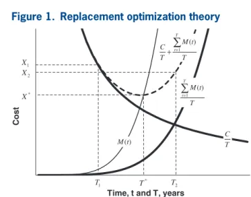
Figure 1 is a conceptual model of average costs familiar to economists. The downward sloping dark curve is the average cost of replacement, which decreases with T. The upward sloping dark curve is the average cost of repairs, which increases with T. The dotted curve is the total average cost of repair and replacement, which is the sum of the two dark curves. Unlike M(t), these curves represent averages over a long period of time, and over a large number of replacements. The formulae shown on the graph show the algebraic relationships of these curves to M(t), C, and T. We use summations rather than integrals due to the fact that M(t) would probably be measured in discrete annual amounts.
The most important feature of this graph is that for increasing M(t), the total average cost of repair and replacement (the dotted curve) is minimum at T*, which corresponds to a total average cost of repair and replacement of X*. It also illustrates that if times other than T* are chosen for replacement, that total average costs will be higher. The efficient time for its complete and utter replacement with a new one.
Few actions are as expensive. To understand the rea-sons for replacement, it is useful to remember that the opportunity costs associated with keeping an old asset (not having the newer version of the like asset) usually rise as the asset ages. This is the natural con-sequence of aging machinery components and envi-ronmental factors, such as energy costs and advances in technology. At some threshold of these costs, a decision to replace an entire asset may be preferable to one of continuing to pay for rising opportunity costs. We will initially focus only on unscheduled repair costs, in keeping with our service contract analogy, but will then show that our models encom-pass any actual expenses and opportunity costs that influence the replacement decision.
Let us initially define M(t) only as the variable cost of repair at time t. M(t) is the annual variable repair cost in calendar year t. Later, we will expand this definition to mean all the opportunity costs asso-ciated with an individual asset that are above and beyond the operating costs of having the latest, new-est, like asset. These variable costs are the additional costs for a company to repair an item of equipment beyond its fixed costs. Variable costs vary with the frequency of equipment failures, but fixed costs do not. An example of a variable cost of repair is the cost of new components and labor to install them, and is contingent on the occurrence of an equipment failure. An example of fixed costs is the cost of rou-tine, scheduled, preventive maintenance.1
A company may also have lower variable costs for a given level of repairs because of its degree of dependence on fixed costs to accomplish the same repairs—for example, the level of on-the-job train-ing given to its maintenance staff, or the investment in permanent tools needed to perform maintenance functions. We loosely define these differences in
1Although there is a relationship between the level of routine,
preven-tive maintenance and the frequency of equipment failures, this does not change the fact that preventive maintenance can be regarded as a fixed cost. The question of choosing an optimum level of preventive mainte-nance is separate from the replacement timing question under analysis, and a focus of a field called enterprise asset management (EAM).
Cost
Time, t and T, years M(t)
T M(t)
T
t=1
T C T
M(t)
T C
+
T
t=1
2
X
1
X
*
X
*
T
1
T T2
∑
∑
4. A financial model for physical
asset replacement
A second conceptual approach is to think of replacement as an option that should be exercised at the optimal time, T*. In this model, we compare the present value of M(t) evaluated at T* in perpetuity, to the present value of all future repair and replace-ment costs, resulting from a replacereplace-ment at T*, in perpetuity. Repair and replacement are mutually exclusive and complementary options. By deciding to not replace a physical asset today, one is deciding to continue to repair it. By deciding to not continue repairs, one is deciding to replace the asset. For a going concern, there is no third exclusive option. There is also no “do nothing” option with respect to these two alternatives. Therefore, the decision must be exercised relative to each physical asset, individually.
If the variable cost of repairs is increasing, it will cross a certain threshold at time T* at which the pres-ent value of continued repairs at that threshold will exceed the present value of an immediate ment with all its attendant future repairs and replace-ments. Optimal replacement occurs at this threshold value of M(t).
The two first terms on the right side of equation (4.1) represent the present value at replacement time of a perpetuity (due) of replacements costing C occurring every T* years. The third term on the right of equa-tion 4.1 represents the present value at replacement time of a perpetuity of all repair costs repeating every
T* years. The time value of money is represented by a discount rate, i.
∑
( )
= + +( + ) = ( )M T
i C
C is
i M t v is
T
T t
t T
T
* 1
. (4.1)
*
* 1 *
*
Multiplying both sides of equation (4.1) by i gives
∑
( )
= + +( + ) = ( )M T iC C s
i M t v s
T
T t
t T
T
*
1
. (4.2)
*
* 1 *
*
replacement is at T*. Any other replacement time is not efficient.
This figure illustrates the effects of a repair versus replacement policy. If replacements occur before T*, at T1, then the total average repair and replacement cost will be higher than X*, at X1. This results from a surplus of M(t) under M(T*). If replacements occur after T *, at T2, then the total average repair and replacement cost will also be higher than X*, at X2. This results from a deficit of M(t) over M(T*).
Efficient repair versus replacement policy may have a material impact on the earnings of organi-zations that rely heavily on physical equipment to generate revenues. For example, a power utility with $20 billion in machinery and equipment with an optimal lifespan of 20 years would pay 1/20th ×
$20 billion each year in replacements, and perhaps an additional 15% of this amount in repairs, or $1.15 bil-lion. If an inefficient repair versus replacement pol-icy resulted in an additional 10% in excess of X* in total average repair and replacement costs, then this would add $115,000,000 to the organization’s annual operating costs. If earnings were on the order of $1 billion, then this inefficiency could be mate-rial to such an enterprise’s market valuation. This is a hypothetical example, and we do not have docu-mented accounting evidence of the inefficiencies predicted by Figure 1. However, the dollar values and the potential loss of efficiency (see section 6.2) described in the example are realistic.
Figure 1 has two important implications. First, it illustrates the existence of an optimal inter-replacement time. The second implication is the causal relationship between repairs and optimal replacement timing, since the evolution of M(t) determines T*.
with low repair costs (relative to replacement), such as buildings or concrete structures, which explains why most of our discussion on replacement of physi-cal assets focuses on capital equipment.
Since we know little about the function M(t), apart from some gross characteristics discussed below, it is a boon to our analysis that it can be dropped from our determination of the appropriate asset replace-ment time. Decisions for the efficient replacereplace-ment of physical assets can be based on a simple trigger that is easily articulated in policy, or as a contractual per-formance obligation.
If i = 0, then equation (4.2) reduces to equation (4.5):
∑
( )
= + = ( )M T C
T
M t T
t T
*
* * . (4.5)
1 *
The first term on the right side of equation (4.5) equals the average cost of replacement in Figure 1, and the second term on the right side of this equation equals the average cost of repairs in Figure 1, both evaluated at the optimal replacement time, T*. There-fore, the financial model described in equations (4.1) through (4.4) converges with the economic model described in Figure 1, if we ignore the time value of money in both models.
The curves in Figure 1 can be adjusted for the time value of money to obtain the same result as in equa-tions (4.1) to (4.4), but then Figure 1 would lose its simplicity and illustrative power as an economist’s tool for understanding the minimization of average costs. This adjustment would also not affect the two important implications of Figure 1 discussed in sec-tion 3. If this adjustment were graphed, we would notice that M(t) still intersects the minimum point of the adjusted average cost of repair and replace-ment (the dotted curve), just as it does in Figure 1. All curves of Figure 1, except for M(t) would move upward and to the right with an increasing (nonzero) discount rate. We will not create such graphs here, but simply note that equations (4.1) to (4.4) provide the correct threshold values of M(T*), because of their inclusion of the time value of money.
The continued derivation beyond equation (4.2) is provided in the Appendix, but for M(t) exhibiting the kind of convexity shown in Figure 1, most values of
T* typical of capital equipment (i.e., T* > 10 years), and for typical values of i, the right term of equa-tion 4.2 becomes very small, and equaequa-tion (4.2) can be approximated by2
( )
≅ +M T iC C sT
* . (4.3)
*
As T* becomes very large (i.e., T* > 75 years), equation (4.3) can be further reduced and approxi-mated by equation (4.4).
( )
≅M T* iC. (4.4)
Equation (4.4) is simply the discount rate multi-plied by the all-in cost of replacement and represents an observable threshold of increasing M(t) at which the replacement decision is optimal. The equation becomes an equality as T* or i, or both, become large. Equations (4.3) and (4.4) are very handy rules of thumb, and are reasonably accurate for replace-ment decisions for most types of physical assets with lifespans longer than 10 years. In equation (4.3), T* is an a priori estimate of the expected useful life of the physical asset. Equation (4.4) requires no such estimate of the expected lifespan of the physical asset, but would not be appropriate for short-lived assets, such as information technology or vehicles.
This conceptual model has its own interesting implication. If M(t) never exceeds this threshold, then replacement will never occur. In such a situation, there will never be a rational time in which the enterprise should replace the physical asset. This may be the case for an enterprise with a very low marginal cost of repair. It is also the case for many types of assets
2The statements about the approximate nature of these relationships can
nite. In other words, the cash flows under consider-ation only have to be as long as the expected lifespan of the replacement asset, not in perpetuity, in order for the trigger expression in equation (4.10) to be true.
For typical asset lifespans, the threshold value of
M(t) is most sensitive to estimates of the discount rate and the all-in replacement cost (which are eas-ily estimable), less sensitive to errors in the a priori estimate of lifespan, and virtually insensitive to the (unknown) form of the function M(t).
4.1. A broader interpretation of
M
(
t
)
In the above conceptual models, M(t) was defined as the calendar year variable cost of repairs for a physical asset at time t. This interpretation is usu-ally consistent with the scope of responsibility in an extended service contract. The service provider for such a contract is usually not obliged to replace an item of capital equipment simply because a newer, more efficient version of the same capital equip-ment emerges in the market. However, the owner of the asset internalizes all economic costs associ-ated with it, and may wish to expand the definition of M(t).
A more general interpretation of M(t) would be that it represents the calendar year cost (in year t) of holding an old physical asset. By holding an old physical asset (instead of replacing it) the enter-prise may pay not only for increasing repairs, but expected revenue losses due to increased frequency of downtime of aging equipment, or for the oppor-tunity cost of lower operating expenses associated with new, more technologically advanced replace-ment equipreplace-ment. Such opportunity costs can be objectively quantified as savings in operating and routine maintenance costs. Since technology gen-erally improves, these opportunity costs increase, which is consistent with our assumption of increas-ing M(t) in our model.
For those replacement assets that are capitalized, even the opportunity cost of not realizing the tax shelter from depreciation of a new asset can also be considered a constituent of M(t).
Another way to approach this problem derives from personal experience. A few years ago, I replaced an old car. It had been in the shop several times that year for unrelated repairs, and seemed to continue a trend of increasing costs that had begun a few years earlier. The maintenance costs, I reasoned, were becoming a significant fraction of what I would pay annually for a loan on a new car, and without all the hassle. Of course, the annual amount of such an imaginary loan would depend on its term, but the number I had in mind for comparison was for the longest pos-sible loan, perhaps approaching the amount of time I might own the next car. My annual maintenance costs were becoming an ever-increasing proportion of the annual amount that would be paid for this loan (equation (4.6) below).
=
Amount C aT
(4.6)
*
Then, with some algebra:
= C
v sT T
(4.7)
* *
( )
=C +i
s
T
T
1
(4.8)
*
*
[
( )]
=
+ −
+
C
i i
i
s s
T
T T
1 1
1
(4.9)
*
* *
= +
= +
C i
s iC
C s
T T
1
(4.10)
* *
infi-in t, are random. Repair costs are fortuitous by virtue of their causation by random physical factors, such as breaking, snapping, short-circuiting, wearing, rup-ture, or fouling. The very propensity of a physical asset to require repairs (a measure of its quality) is a function of factors beyond the enterprise’s control. For example, was the physical asset produced dur-ing a labor strike at the factory? Technology change, reflected as opportunity cost in M(t), is an uncon-trolled external factor, which can also trigger the replacement decision. The rising opportunity cost created by unforeseen technology advances is for-tuitous and beyond the control of the enterprise pursuing a policy of efficiency.
Since replacement times are determined by a sto-chastically increasing M(t), and the optimal replace-ment time depends on a threshold of M(t), then the time until that threshold is crossed is also random. Because the constituent costs of M(t) are fortuitous, efficient replacement costs are also fortuitous in a sense similar to the fortuity of death benefits. Repairs and replacements, if executed efficiently, are both examples of unscheduled maintenance. Any attempt to schedule or plan replacements will generally not be efficient.
M(t) increases and approaches a threshold from underneath much in the same way that an aggre-gate excess of loss treaty attachment point might be approached over time. Measuring M(t) and knowing when it crosses the threshold value can be difficult, particularly if we wish to use equation (4.3) as a con-tractual trigger for replacement. The use of moving averages of M(t), in order to dampen observed fluc-tuations, and avoid making premature replacement decisions, can solve this problem.
The perpetuity equations above assumed that replacements are evenly spaced apart in time, but the random nature of M(t) invalidates this assumption. Since inter-replacement time is a random variable, replacements are a stochastic stream of events. The present value of a stochastic stream of cash flows is not equal to the present value of a regularly spaced (scheduled) stream of cash flows, as was assumed There are probably potential constituents of M(t)
that are impossible to measure objectively. For exam-ple, how does one put a value on “new car smell” when making a decision to buy a new car? In an industrial setting, these constituents are, or at least should be, selected on a more rational basis. Having the flexibility to explicitly define the constituents of M(t) actually allows elimination of subjective, even behavioral, constituents that have the poten-tial to contribute to decisions that are irrational with respect to the goal of maximizing enterprise value. An example of this would be deferral of replace-ments for the sake of short-term profitability or a manager’s bonus.
There are probably also constituents of M(t) that are difficult to quantify. For example, the expected revenue lost due to increasing downtime of an aging physical asset. These costs, although difficult to mea-sure, still exist. Such obstacles are also present in tra-ditional capital expenditure planning methods often used in an asset replacement decision.
In theory, any calendar year cost of not replacing old equipment that would be considered under a tra-ditional capital budgeting method could be monitored as a constituent of M(t). Because of the increasing prevalence of individual physical asset accounting systems, repair costs of individual assets are now being regularly tracked and updated. Such informa-tion systems can easily be adapted to include current opportunity costs, and any other objectively measur-able economic constituents of M(t). Such costs can be monitored by engineers, and the accuracy and documentation of that information could become an increased focus of their expertise.
By broadening the definition of M(t), we expand our theory to balance all possible operating expenditures against replacement costs or capital expenditures.
4.2. The random nature of
M
(
t
)
tional events, and not regular phenomena that occur over the lifespans of each replacement.
The assumption of convexity in M(t) as depicted in Figure 1 is important, since it means that most of the M(t) costs occur late in the life of a physical asset, and therefore are heavily discounted in equa-tion (4.2). Convexity in M(t) is what helps us to eas-ily drop it from the determination of the approximate replacement threshold value of M(t) in equation (4.3).
4.5. The nature of
i
By broadening the definition of M(t) in section 4.1, the trigger for economically optimal replacement of a physical asset given by equation (4.3) now resem-bles the usual process of capital expenditure plan-ning in which the net present value of all future costs operating old physical assets are compared to that of new ones.
Since we now understand the preceding equa-tions to be an expression of the traditional capital budgeting process in the context of renewal, and we are considering alternative uses of a firm’s free cash flow, we can conclude that the discount factor used in the above perpetuities is the (real) cost of capital of the entity making the replacement decision.
4.6. Summary of assumptions
concerning
M
(
t
)
The assumptions concerning M(t) were made in order to create an argument from which to draw use-ful conclusions. The assumptions are summarized as follows:
• M(t) is comprised of variable repair costs, but must also include opportunity costs of improved tech-nology, expected loss costs due to downtime, and any other cost that would normally be considered under a traditional capital budgeting method when making a replacement decision.
• M(t) increases, and does not return to a value below the threshold value at which replacement is required, once this threshold is crossed.
• M(t), although increasing, is random, and approaches the threshold value requiring replacement, much in our financial model. However, the impact of this
idealization on the accuracy and implications of the equations above is minimal, and merely represents a further refinement of our analysis to be handled below.
4.3. Ever-increasing
M
(
t
)
Figure 1 shows that M(t) increases, and is assumed to never return to a level below M(T*). This assump-tion simplifies the financial model described earlier in this section 4, and is based on historical experience that all of the so-far mentioned constituents of M(t) generally increase over time. There may be excep-tions to this. Repair costs, for example, can decrease after a period of high frequency of repairs. This is especially true for arrays of identical components that comprise a single physical asset, which can create periodic concentrations of repair costs over time, or for relatively simple machines. However, rising opportunity costs associated with advancing technology are usually not reversible.
4.4. The convexity of
M
(
t
)
In Figure 1, M(t) is shown to have convexity. That is, costs seem to increase at an increasing rate over time. This is largely anecdotal, but there is a theo-retical basis for this. Since most equipment compo-nents follow time to failure distributions that have an increasing force of mortality over time (i.e., the Weibull distribution), one would expect an aggrega-tion of such components to exhibit the same progres-sion of repair frequency, thus convexity, as that seen at the lower percentiles of such a distribution. Equip-ment that requires repairs at an evenly increasing rate over time would be considered to be of very poor quality.
excep-∑
( ) ( ) ( ) ≥ + + + =M t iC E C s
i M t v s T T t t T T 1 (4.7.3) * * 1 * *
The phenomenon of M(t) intersecting the mini-mum is also preserved for the actuarial present value as it was for the dotted curve in the Figure 1. This is because it is possible to capture the randomness of the replacement time simply with a risk-adjusted cost of capital instead of i, and we have already determined that the phenomenon of M(t) intersecting the minimum is preserved for equation (4.2).
Approximation 1:
As we first noted after equation (4.2), the right-most term inside the brackets is then assumed to equal zero.
( )≥ + +
M t iC E C sT
0 (4.7.4)
*
We do this only to get rid of that term, since it cannot be easily evaluated using objective data, and since its value is very small compared to the other terms in the equation. M(t) does not follow a deter-ministic process as depicted in the above graphs; rather, it follows a stochastic process, and the elimi-nated term would require considerably more historic data to evaluate than can be reasonably obtained in practice. A possible range of values of this term can be obtained through scenario testing, and since the values are usually very small compared to the other terms, this approximation slightly understates the right side of the inequality.
Then, dividing both sides by C,
( )≥ +
M t
C i E sT
1 . (4.7.5) * Approximation 2:
∑
= = EsT i sT N N
i
1 1
(4.7.6)
* 1
the same way in which the attachment point of an aggregate excess of loss treaty is approached. • M(t) has convexity, as depicted in Figure 1.
These idealizations broadly describe the time-dependent nature of factors usually considered in a replacement capital budgeting exercise. They are not always true, but experience has shown that they are usually the rule rather than the exception. These assumptions are probably always true for a large subset of physical assets, such as capital equipment.
4.7. Stochastic considerations
of the model
Expressions (4.1), (4.2), and (4.3) do not provide guidance for when to replace individual assets, since they assume that all assets have identical lifespans. As we have described in section 4.2, assets (locomo-tives, wind turbines, vehicles, etc.) are not replaced punctually at some average lifespan.
First, let us show Equation (4.2) as an inequality, since we are really concerned with timing a decision with the rising M(t), so anytime M(t) is greater than (or equal to) the right side of the equation is when to replace the asset. When the following inequality is satisfied, we must replace the asset in order to mini-mize the present value of all future costs associated with the asset:
∑
( )
( )≥ + + + = ( )
M t iC C s
i M t v s T T t t T T 1 (4.7.1) * * 1 * *
Then, since the time to replacement is random, we take the expected value of the right side of expres-sions (4.1) and (4.2). We want to do this, since we are interested in minimizing the expected value of the present value (the actuarial present value) of all future costs associated with each individual asset and its successors.
∑
( ) ( )≥ + + + ( ) =M t E iC C s
or even better, a homogeneous ensemble of similar vehicles in a fleet owned by the same enterprise. As soon as this inequality is satisfied for an individual asset, one must replace the asset in order to minimize costs for the entire class of assets.
It is important to note here that, since the sampled empirical ages affect the calculation of the threshold value, they also affect the values of newly generated empirical ages. Asset mortality data generated by the model is also fed back into the model, since it newly characterizes the mortality of the class. Therefore, this model is iterative. The model will converge to a steady state, but the selection of seed values for
T1, T2, T3, . . . , TN should be done with the goal of shortening the calibration period.
4.8. Principles of physical
asset replacement
The conclusions from the application of simple financial mathematics to the above assumptions about the nature of M(t) can be summarized by the following three principles:
1. There is only one instant in time that an asset must be replaced in order to minimize the present value cost impact to the enterprise.
2. This efficient instant is observable, and a func-tion of both the owner’s cost of capital and readily obtainable current calendar year information. 3. The time to this efficient instant is random. It may
be infinite.
The above principles imply that efficient physical asset replacement is a life contingency problem. The advantage of having an easily calculable and objective trigger for economically optimal replacement is man-ifested by the ability to make prompt decisions that are ruthless with respect to the goal of minimizing the overall net present value cost impact to the enterprise. A threshold value, based on readily observable calen-dar year information, makes it possible to base con-tractual replacement obligations on events that cannot be manipulated by either party to such a contract. The advent of individual physical asset accounting systems makes it easy to track all types of costs associated with where T1, T2, . . . , TN, are empirical ages at the time of
replacement (asset mortality data) from a homoge-neous class of assets.
This assumes that the expected value of the above term is simply equal to the average of the term evalu-ated over N empirical observations of time to replace-ment of similar assets. Although a close approximation, it is really the interreplacement time at each future replacement that is random, not an identical value of interreplacement time for all future replacements. This approximation tends to slightly overstate the right side of the inequality.
The inequality now looks like this:
∑
( )≥ + =
M t
C i i sT N N
i
1
. (4.7.7)
1
Considering the two approximations we have made so far,
( )
( )
+ = β
Approximation1 slightly understates the right side
Approximation 2 slightly overstates the right side
The errors due to Approximations 1 and 2 are small, and occur in opposite directions. They approximately cancel each other out, but we will call their sum β, and include it in the model. This value is a small error term that can be evaluated through simulation and judgment. The appropriateness of these two approximations will require further analysis on a case-by-case basis.
The model now looks like this, and can be broken down into these parts:
M T
C i i sT N N
i
∑
( )
≥ +
+ β
( )
=
* 1 (4.7.8)
Objective
Empirical Subjective
Individual Asset
1
Entire Class Error
wide policy or contractually. Other capital expendi-ture decision making tools, such as payback period, internal rate of return (IRR), and net present value (NPV), are described in introductory finance texts. Often, the authors of those texts express a preference for the NPV method. The equivalent annual cost (EAC) method also incorporates the time value of money, and is used as a means of comparing invest-ments with different time horizons, such as asset lifespans.
These are all excellent tools for evaluating new capital investments or projects. They are flexible, and can be used to simultaneously evaluate multiple capital investments, particularly those with a finite horizon. However, in our situation, the initial capital investment is a sunk cost, and the asset is already on the balance sheet generating revenue. Physical asset renewal is distinct from initial capital investment in that there are always the same two mutually exclu-sive options (see beginning of section 4) under con-sideration, and timeliness of the decision between these two options is important.
An enterprise-wide policy based on the triggers described by equation (4.7.8) recognizes the impor-tance of timeliness in the asset replacement decision. However, other capital budgeting methods are used in a manner consistent with planning for new capi-tal investment. These traditional methods are purely prospective in that they only recognize that the time to replace an asset has arrived, but fail to account for the fact that the best time to replace the asset may have long passed.
Traditional capital budgeting tools are also rela-tively cumbersome and haphazard tools. They depend on the initiative of line managers, must be created for each project, and are subject to review, second-guessing, and deferral. In the situation of long-lived assets for a going concern, equation (4.7.8) reduces the capital budgeting process to monitoring a pre-determined set of current calendar year M(t) constit-uents, and regular comparison to threshold values. Decisions are made by policy. The only input needed in such a system is the continual data entry of cal-endar year M(t) information, with the decision itself individual physical assets, and makes enforcement of
such a policy or service contract feasible.
4.9. Model interpretation
Because of its iterative nature using feedback, the model of equation (4.7.8) is a process control algorithm, and the process in question is the mortal-ity within entire ensembles, fleets, or homogeneous classes of physical assets. Decisions on individual assets depend on aggregate information (asset mor-tality data) from the fleet to optimize the performance of the entire fleet. One can imagine that the random life distribution defining mortality of a class of assets will not remain stationary, but will migrate in shape and form over time as distributional changes caused by environmental factors, such as advancing technol-ogy or changing energy costs, work their way through an asset population of mixed ages. As these distribu-tional changes occur, the model follows them with the singular goal of minimizing the actuarial present value of all future costs, both capital and operational.
The structure of this model shows that even if the accuracy on the right side of the inequality is not per-fect, the left side always provides a way to prioritize the assets for replacement in order to achieve the minimum of average total cost.
Most of this model is based on objective data that can be easily obtained in practice. M(t) is simply the engineering data which ordinarily goes into this type of analysis, such as energy costs, repair costs, expired depreciation, potential loss costs, potential down time costs, etc. The model also separates the data obtained from the individual asset from the asset mortality data obtained from the entire class of assets. There is a clear role for the art of classifica-tion of assets into homogeneous groups with similar characteristics that affect their mortality.
5. Comparison with other capital
budgeting methods
∑
( )
= + +( + ) = ( )M T iC C s
i M t v s
T
T t
t T
T
*
1
. (4.2)
*
* 1 *
*
In this section, we introduce another interpretation of the terms on the right side of equation (4.2). The sum of these terms represents an equivalent annual level amount in perpetuity, which is minimized at the efficient time T*. For other values of T, the equality in equation (4.2) is not true. In other words, this equiva-lent annual amount, let us call it A(T ), is not equal to
M(T) for values of T other than T*. Equation (4.2) is generalized as follows:
∑
( )
= + +( + ) = ( )A T iC C s
i M t v s
T
T t
t T
T
1
. (6.1)
1
Now we can say that the present value of an effi-cient enterprise policy based on equation (4.2) is equal to M(T*)/i, and that the present value of an (inefficient) enterprise policy based on equation (6.1) (where T is not T *) is equal to A(T )/i. The pres-ent value impact of a transition from an inefficipres-ent policy to an efficient policy would be the difference between the present values of these two perpetuities.
We then assume that a firm is using a 5-year payback approach to justify the replacement of the physical asset, which corresponds to M(t) = 0.2C at replacement time, and if we let i = 4.5%, C = 1000, and describe M(t) using the following polynomial3
( )
= + + + +M t at bt2 ct3 dt4 et5 (6.2)
where the coefficients equal:
a 0.000000000067
b 0.000000001696
c 0.000000037193
d 0.000000780821
e 0.000016087092 being automated. The increased usage of individual
physical asset accounting systems make this a prac-ticable reality today.
6. Value impact to an owner
6.1. Measurability
Asset renewal is generally the result of a traditional capital budgeting process, and, as we have already noted, planned replacement timing generally is not efficient. However, we cannot estimate the magnitude of that inefficiency for any company simply by exam-ining its financial statements, or even from detailed existing accounting data. To the extent that M(t) is not being continuously monitored, and managers are not aware of the threshold indicated by equa-tion (4.7.8), the efficient replacement policy of Fig-ure 1 will generally not be realized.
Although there are now individual physical asset accounting systems which can digitally track all kinds of cost data at the individual asset level, they are not presently being used to record all the constituents of
M(t) described in section 4.1, hence the losses in effi-ciency that are predicted by Figure 1 are not being monitored (continuously or otherwise). Once M(t) is defined and continuously monitored, it would be pos-sible to measure existing deficits of M(t) over M(T*) and any surpluses of M(t) under M(T*) for assets about to be replaced. This would allow approxima-tion of the present value cost impact of a policy that aims to eliminate such deficits and surpluses.
6.2. Magnitude
Earlier, we used an example of a power utility that might be experiencing 10% excess costs associated with machinery and equipment. In that example, we referred only to repair and replacement costs, but we now know that the inefficiency affects any operational costs associated with physical assets. The following analysis provides some basis for that 10% assumption.
In equation (4.2), we equated the calendar year value of M(t) with a set of terms at the efficient
benchmark. The 10% inefficiency assumption used in the power utility example is at the lower end of this range, and may be generous.
7. Distortions on incentives in ISCs
The conceptual models of sections 3 and 4 try to approach capital planning associated with repair and replacement from the rational perspective of the facility owner. Care must be taken in the contract language to insure that the incentives of the service provider enhance and protect the interests of the facility owner.
7.1. Finite term of ISCs
The discussion so far has focused on an analysis of cash flows in perpetuity. This may be true for the owner who views the facility as a going concern. However, ISCs have finite terms, and service pro-viders do not expect to continue repair and replace-ment obligations past the end of those terms. In many cases, the contract term is only about as long as, or low multiples of, the average expected life of capital equipment in a facility.
The finite planning horizon of the service provider could encourage behavior, near the end of a contract term, to defer expensive replacements in favor of continued repairs. These repairs may be less costly to the service provider who is planning to leave the facility soon. The owner may be left with a facility that is functional, but obsolete. In other words, at the end of the contract term, the owner may be left with a facility full of old equipment that needs replacement.
7.2. Whose cost of capital?
In section 4 we derived a rule that tells us that the optimal time for replacement for most types of capital equipment is when increasing M(t) crosses a thresh-old proportional to the product of the cost of capital and the all-in cost of replacement (iC). However, if the cost of capital for a contract holder, who issues municipal bonds, is around 4.5%, the cost of capital for a service provider is 7%, and the cost of capital One can plot equations (4.2) and (6.1) to show
that T * = 22 years, M(T *) = 83 and A(T ) = 89 at
T = 26 years where M(26) = 200. This represents about a 7% increase in the present value cost impact due to the inefficient 5-year payback replacement policy. Because of the extreme convexity of M(t) in this example, a 5-year payback policy that is not prompt, resulting in an additional deferral of only 4 more years (to T = 30), would result in A(T ) = 104, which repre-sents about a 25% increase in the present value cost impact due to an inefficient replacement policy.
If we replace the polynomial used for M(t) by a straight line (no convexity):
( )
=M t 3.882 .t (6.3)
Performing the same calculations based on equa-tions (4.2) and (6.1), we show that T* = 23 years,
M(T*) = 90 and A(T ) = 121 at T = 51 years where
M(51) = 200. This represents about a 34% increase in the present value cost impact due to an inefficient replacement policy. Because there is no convexity of
M(t) in this example, a policy resulting in additional deferral of a few more years would not result in a significant increase in the present value cost impact due to an inefficient replacement policy.
The very existence of ISCs creates a precedent. It demonstrates that it is possible to transfer the risk of uncertain future capital expenditures associated with new or existing facilities between entities. The demand for ISCs stems from the following reasons:
• A desire to assign unpredictable long-term repair and replacement costs to the party that has the greatest ability to control them, namely, the builder and operator of the facility.
• To assure that needed funds are promptly made available for repairs when machinery breaks down. • To accelerate the timely repair or replacement
of equipment from the standpoints of safety and reliability.
Although not the original intent, extended service contracts for facilities and infrastructure have achieved the following collateral purposes:
• As a mechanism to save earnings during an ini-tial period of low maintenance costs (and higher profitability) on new facilities, for a later period of higher maintenance costs (and lower profitability) as the facility ages.
• To have the funds necessary to ruthlessly replace equipment at the economically optimal time, and eliminate incentives to defer expensive replace-ment of equipreplace-ment in order to enhance short-term profitability.
• ISCs can have very long-tailed payout patterns because of the longevity of capital equipment. They may present an opportunity to earn invest-ment income, and benefit from deferral accounting and tax treatment.
As we have mentioned, insurers are not involved in underwriting these risks. Nor have we found non-insurance entities willing to cover these long-duration repair and replacement obligations under a stand-alone commercially available product. There are two market failures, which may explain why this is so:
• Information asymmetry—For an old facility, the owner of the physical assets knows far more about the age, condition, and maintenance history of for a manufacturer who relies mostly on equity
capi-tal is 10%, then there is clearly a mismatch of opti-mal replacement timing implied by equations (4.3) or (4.4). Entities with the higher cost of capital will rationally defer replacement decisions, compared to those with the lower cost of capital. Unless there is an objective contractual trigger for replacement that explicitly recognizes which cost of capital to use, this mismatch may have a deleterious impact on the contract holder’s interests.
Although we believe that a replacement trigger based on equation 4.7.8 is the more practical way to protect an owner’s interests, ISCs can have pro-visions to stipulate a required physical condition of the facility at the end of the contract term. This is an attempt to force repair versus replacement decisions to be made in a way so that the facility, at the end of the contract, would be in a condition identical to that had the owner been in charge of all such decisions.
7.3. Systematic incentive
to defer replacement
Wendling (2012) outlines a simulation experi-ment to demonstrate how managers, who consider the retirement and replacement of individual assets in isolation, may have rational incentives, due to risk aversion and uncertainty, to defer the replacement of assets past a time optimal from the perspective of the shareholder who owns the entire portfolio of such assets.
8. Managing capital expenditures
9. Potential impact on
tax deductibility
Our discussion so far has focused on an enter-prise policy to increase operational efficiency, but has inadvertently led to an understanding that effi-cient physical asset replacement costs depend on the occurrence of specified, uncertain, future events. Efficient asset mortality results in volatile future cash flows, so there is an interaction between efficiency and fortuity. Efficient replacement costs are fortu-itous in a sense similar to death benefits. Although the tax deductibility of prepayments for future capi-tal outlays, particularly in the aforementioned cap-tive arrangement, is untested, when fortuity is truly present and when there is a valid business purpose (efficiency and risk transfer) for such prepayments, it influences the discussion of tax deductibility, at least theoretically.
According to Section 162(a) of the Internal Rev-enue Code (26 U.S.C. § 162(a)), an expense must first be deemed necessary and ordinary, among other requirements, in order to be considered deductible for federal income tax purposes. One can argue that an extended service fee based on the contractual trigger described in equation (4.7.8) is necessary, both from the standpoint of transferring risky (volatile) cash flows and for creating efficiency. In other words, there are two legitimate reasons for such an expense. These fees might also be considered ordinary, since extended service contracts already exist to repair and replace physical assets at different levels of aggrega-tion. The only thing which sets the ISC apart from a conventional service contract is that it may replace physical assets up to the highest level of aggregation for the entire plant, and over much longer periods of time than most other types of extended service con-tracts. To the extent that such contracts already exist, their fees are ordinary.
In the Internal Revenue Service (IRS) revenue ruling 2007-47, the IRS does not allow deductibility for arrangements that are little more than prefunding of future known costs. It is evident that the subject of fortuity has a bearing on whether or not a payment capital equipment than an outside provider of an
extended service contract, thus inviting adverse selection.
• Routine maintenance monitoring—For both new and old facilities, the inability of an extended service contract provider to monitor an owner’s compliance with OEM recommended routine maintenance re-quirements, thus encouraging moral hazard mani-fested by lapses in costly preventive maintenance.
The second of these problems is probably the most substantial one. It is due to a highly heterogeneous mix of equipment typical at an industrial facility. Each type of equipment will have different OEM instructions regarding scheduled, routine, preventive maintenance to minimize future unscheduled repairs. Non-compliance with such maintenance instructions cannot always be detected after the fact. Routine maintenance involves many factors such as lubrication, testing, changing of wearable components. These activities would be difficult to monitor and verify by a third party extended service contract provider, unless the service provider is also providing the rou-tine maintenance services.
Although this coverage is not commercially avail-able outside of the total suite of services described in section 2, the ISC could theoretically have vitality in a self-insurance model, which might be unaffected by these market failures. For example, an ISC, if admin-istered through a captive entity, could insure the availability of funds and provide the contractual trig-ger for timely replacement of assets in order to gain the efficiencies predicted by the economic theory.