Transportability of Trial Results Using Inverse Odds of Sampling Weights
Daniel Westreich*, Jessie K. Edwards, Catherine R. Lesko, Elizabeth Stuart, and Stephen R. Cole *Correspondence to Dr. Daniel Westreich, Campus Box 7435, McGavran-Greenberg Hall, Department of Epidemiology, Gillings School of Global Public Health, University of North Carolina at Chapel Hill, Chapel Hill, NC 27599 (e-mail: [email protected]).
Initially submitted August 18, 2015; accepted for publication December 7, 2016.
Increasingly, the statistical and epidemiologic literature is focusing beyond issues of internal validity and turning its attention to questions of external validity. Here, we discuss some of the challenges of transporting a causal effect from a randomized trial to a specific target population. We present an inverse odds weighting approach that can easily operationalize transportability. We derive these weights in closed form and illustrate their use with a sim-ple numerical examsim-ple. We discuss how the conditions required for the identification of internally valid causal ef-fects are translated to apply to the identification of externally valid causal effects. Estimating effects in target populations is an important goal, especially for policy or clinical decisions. Researchers and policy-makers should therefore consider use of statistical techniques such as inverse odds of sampling weights, which under careful as-sumptions can transport effect estimates from study samples to target populations.
causal inference; epidemiologic methods; external validity; generalizability; transportability
Abbreviation: HIV, human immunodeficiency virus.
Large randomized trials with complete compliance and no missing data provide internal validity in expectation as a matter of design (1). However,externalvalidity with respect to a specific, investigator-defined target population is not similarly provided (2–7). Unless the study sample (PS) was sampled at random from the target population (PT), there is no expectation of exchangeabil-ity of the study sample and the (again, investigator-defined) target population. Yet nearly all trials are conducted among study sam-ples that are not sampled at random from the target population, for reasons of either design (e.g., to maximize statistical power, a trial is conducted among those at highest risk of an outcome) or hap-penstance (e.g., if persons who exhibit health-seeking behaviors participate in the trial at higher frequencies than others). In these cases, despite having an internally unbiased sample average treat-ment effect, that sample average treattreat-ment effect may differ from the average treatment effect in the target population.
Given that we have internally valid trial results, we often wish to ask the question: What would happen had this trial been con-ducted in another, external population—the target? Above we suggested that we might want to ask about the causal effect of the treatment in the populationfrom which the study population was sampled(albeit perhaps nonrandomly); we also might wish to address the causal effect of the treatment in a target population
distinct from the study sample, that is, one which is partially or completely nonoverlapping with the study sample. In this latter case—such as when we have a randomized trial and wish to infer a causal effect in a target population—the question can be framed as one of direct standardization to the external target pop-ulation. As a distinction of language, and to be consistent with the evolving literature on this topic, we refer to the former case (where the study sample is a subset of the target population) as a problem of“generalizability,”and to the latter case (where the study sample isnota subset of the target population) as a prob-lem of“transportability.”
=
( = | ) ( = | ) ×
( = )
( = ) =
= W
P S Z
P S Z
P S
P S S
S
0 1
1
0 , 1,
0, 0,
i
i i
i i
i
i
i
i ⎧
⎨ ⎪
⎩⎪
whereSi,Zi, andiare as described above. The weight for individ-ualiis 0 if they did not participate in the study. Otherwise, thefirst term of the weight is the inverse of the ratio of an individual’s probability of being in the study sample as opposed to the target population (hereafter“being sampled”), conditional onZidivided by theirZi-conditional probability ofnotbeing sampled—that is, the inverse of theirZi-conditional sampling odds. The second part of the weight is the ratio of theunconditionalsampling probability to theunconditionalnonsampling probability—that is, the uncon-ditional sampling odds.
We note that this approach differs from the inverse probabil-ity (rather than odds) of selection weights; the latter method, described by Cole and Stuart (4), is appropriate when the study sample is a subset of the target population (i.e., for generaliz-ability rather than transportgeneraliz-ability). Inverse odds weights are appropriate when the study sample and target population are nonoverlapping; if we consider“being in the study sample”to be a kind of treatment, this method is analogous to weighting for the average treatment effect in the untreated in nonexperi-mental studies (11,12).
NUMERICAL EXAMPLE
To aid intuition around this method, consider a hypothetical trial of assignment to a new antiretroviral therapy regimen for human immunodeficiency virus (HIV) compared with assign-ment to a reference regimen, for the outcome of virological fail-ure at 1 year, conducted in HIV-positive people living in the United States. Suppose thestudy samplefor the trial comprises 2,000 participants, 1,000 with single covariateZ=1 and 1,000 withZ=0. Among participants withZ=1, the risk difference is−0.2 (novel treatment is protective against failure); among participants withZ=0, the risk difference is 0.0 (no effect of intervention). The crude sample average causal risk difference is therefore−0.1, a simple average of the 2 strata.
Ourtarget population(alternately, a random sample from our target population) comprises 2,000 persons living with HIV in the United States, of whom 80% haveZ=1 and 20% haveZ= 0. In this very simple case, we can hand-calculate the (target) population average causal effect in our external setting as 0.8× (−0.20)+0.2×(0.00)=−0.16. In real data, we would need to use model-based approaches to account for the joint distribution of multiple continuous and categorical variables.
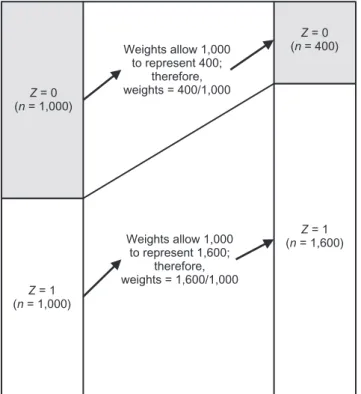
We concatenate the trial data (n=2,000; 50% withZ=1) with the target population (n=2,000; 80% withZ=1), obtaining a combined population of size 4,000, including 2,600 (65%) withZ=1 and 1,400 (35%) withZ=0. We proceed by estimatingO(S=1|Z)=P(S=1|Z)/(1−P(S=1|Z)), which in this case is (1,000/2,600)/(1−1,000/2,600)=1,000/1,600 whereZ=1 and (1,000/1,400)/(1−1,000/1,400)=400/1,000 whereZ=0. We would use these odds to calculate a weighted pseudopopulation of 1,600 persons ((1,000× 1,600/1,000)= 1,600) forZ=1 and 400 persons ((1,000×400/1,000)=400) Previously,ColeandStuart(4)introducedinverseprobability
weights for quantitative generalization of trial results, but they didnotexplainhowtooperationalizethisapproachorwhether their approach was applicable to problems of both generalizabil-ityandtransportability.Morerecently,BareinboimandPearl(3) highlighted several key distinctions between generalizability and transportabilityandintroducedamethodforderivingatransport formula, which relies on a detailed understanding of the causal relationshipsamongallrelevantvariables.Hereweintegrate these 2 methods to introduce an approach to quantitative trans-portabilitywhichmaybesimplertoimplementthanthe trans-port formula.
Abriefadditionalnoteonterminology:WhereColeand Stuart refer to inverse probability of selectionweights (4), we
refertoinverseprobabilityofsamplingweights.Wenote, how-ever, that in many (perhaps most) cases the study subjects were probablynotformallysampled,andwedonotwishtoimplyso with the use of that term; rather, we simply obtain a study sample throughsome(perhapsunclear)mechanism.Forsimplicity,we assume that once a study sample has been enumerated, treatment israndomizedandfollow-upiscomplete,sothatthereisno con-founding bias in expectation and no additional missing data or selectionintotheanalyticalsample(andthereforenoselection bias as a problem of internal validity).
METHODS
Preliminaryissuesandnotation
Sampling (S) might relate to covariates (Z) in several ways, includingScausingZ(orSindicatingdifferencesindistributions of Z), Z causing S, and both S and Z being caused by some addi-tional variable U; here we restrict our attention to the first of these cases, which is closely related to Bareinboim and Pearl’s term “transportability” (3). Weassumethatthe epidemiologisthas conducted a study and wishes to transport the effect estimate fromthatstudysampletoanexternaltargetpopulation.For con-venience, we assume that information on the same set of covari-ateshasbeencollectedinthestudysampleandtargetdata,and that the epidemiologist has concatenated the 2 data sets.
In the following, i indicates a participant index i = 1, 2, . . . n, n + 1, . . . N such that the study sample comprises n participants and the target population N − n participants; study participants are designated Si= 1, while individuals in thetargetpopulationaredesignatedSi= 0;andZiisavector of pretreatment covariates for participant i(see the Discus-sion section for comments on components of Z). Yiaindicates the potential outcome under some specific treatment A = a forparticipanti.
Method
OurgoalisestimationofP Y( ia= 1|Si= )0,theriskofthe outcomeunderaparticulartreatment(a)inthetargetpopulation. In the Appendix, we use the transport formula to derive a set of
forZ=0; we would then calculate the weighted risk difference as (1,600×−0.2+400×0.0)/(1,600+400)=−0.16.
This estimate coincides with the common-sense simple weighted average we derived immediately above. In addition, these inverse odds weights coincide with the intuitive explana-tion of how individuals from the study sample ought to be weighted so as to represent individuals in the target popula-tion, as shown in Figure1. Notably, increasing or decreasing the size of the target population has no impact on thefinal esti-mate, which is not necessarily the case in the method proposed by Cole and Stuart (4).
DISCUSSION
Typical epidemiologic and biostatistical analyses emphasize internal validity of causal effects, but (as others have noted (13,
14)) a causal effect without a specified target population is poorly defined. In practice, study samples for randomized trials are rarely sampled at random directly from the target population; indeed, because consent is an ethical necessity for enrollment in a clinical trial, trial participants are effectively never a random sam-ple of the target population. Yet this is the premise that underlies the assumption of unconditional generalizability or transportabil-ity between the study sample and the target population—a fre-quent (if informal) claim in randomized trials. In contrast, the methods discussed and presented here allow us to relax this ques-tionable premise: We no longer assume that the results from the study population are unconditionally transportable from the study
sample to an arbitrary target population; rather, we assume that they are transportable conditional on variables in our model.
Some people may be uncomfortable with our assumption of conditional transportability, perhaps because herein we are explicit about assumptions that are typically hidden within vague statements about how“representative”the study sample is without addressing the questions 1) representative of what tar-get population? and 2) representative according to which charac-teristicsZ? There is a useful conceptual parallel here with the assumption of exchangeability between treated and untreated subjects for internal validity in an observational setting. The as-sumption of unconditional transportability is similar (but not identical) to the assumption of unconditional exchangeability (e.g., the causal effect is unconfounded), while the assumption of transportability conditional on variables in the model is similar (but again not identical) to the notion of conditional exchange-ability (e.g., the causal effect is unconfounded conditional on a set of confounders).
These parallels are useful in considering the contents ofZ. In earlier work, investigators have variously describedZas com-prising all effect-measure modifiers (5) or as having components identifiable from causal diagrams (3,7,15). The clearest guide-line is thatZshould beS-admissible (16)—that is, thatZshould include pretreatment covariates sufficient to d-separate sampling and the outcome variable (3). This guideline is analogous to that of selecting variables for d-separation of the exposure and out-come variables for internal validity.
As with conditional exchangeability for internal validity, condi-tional transportability of external validity carries with it addicondi-tional assumptions: namely, positivity (9) and correct model specifi -cation. For transport-positivity to hold, the probability of being included in the sample must be greater than 0 for participants in all strata defined byZin the target population. This assumption is necessary so that theZ-specific probability of the outcome esti-mated in the study can“stand in”for theZ-specific probability of the outcome in the target population (seeAppendix). Of course, as with positivity for internal validity, transport-positivity may be replaced by making additional assumptions (e.g., smoothing under a parametric model). As noted elsewhere, additional condi-tions are necessary for transportability—specifically, similar pat-terns of interference and similar versions of treatment between the study sample and the target population (5).
The concerns about external validity discussed here are highly relevant to observational studies as well as to trials. The results of a trial are frequently, naively assumed to be transportable to a tar-get population. Just as often, however, an epidemiologist assumes that observational cohorts are more representative of the target population and thus that there is less need to evaluate transport-ability directly (much less to identify the target population explic-itly). In fact, the transportability of observational studies to a particular target population of interest is not guaranteed and must be evaluated carefully.
In many clinical trials, external validity is considered only an afterthought; however, consideration of both internal valid-ity in the study sample and external validvalid-ity in a target popula-tion is crucial to providing evidence which will best improve medicine and public health (13,17). Quantitative approaches to transportability, such as the one described here, are straight-forward and should be applied more widely.
Z = 1 (n = 1,000)
Z = 0 (n = 1,000)
Z = 1 (n = 1,600)
Z = 0 (n = 400) Weights allow 1,000
to represent 400; therefore, weights = 400/1,000
Weights allow 1,000 to represent 1,600;
therefore, weights = 1,600/1,000
Figure 1. Concepts of weights to map from a study sample with
ACKNOWLEDGMENTS
Author affiliations: Department of Epidemiology, Gillings School of Global Public Health, University of North
Carolina at Chapel Hill, Chapel Hill, North Carolina (Daniel Westreich, Jessie K. Edwards, Stephen R. Cole);
Department of Epidemiology, Bloomberg School of Public Health, Johns Hopkins University, Baltimore, Maryland (Catherine R. Lesko); and Departments of Mental Health, Biostatistics, and Health Policy and Management, Bloomberg School of Public Health, Johns Hopkins University, Baltimore, Maryland (Elizabeth Stuart).
This research was supported by the Eunice Kennedy Shriver National Institute of Child Health and Human Development and the Office of the Director of the National Institutes of Health (award DP2-HD084070) and the National Institute of Allergy and Infectious Diseases (grant R01 AI100654).
We thank Dr. Michael G. Hudgens for expert advice on the preparation of the manuscript.
The content of this article is solely the responsibility of the authors and does not necessarily represent the official views of the National Institutes of Health.
Conflict of interest: none declared.
REFERENCES
1. Hernán MA, Hernández-Díaz S. Beyond the intention-to-treat
in comparative effectiveness research.Clin Trials. 2012;9(1):
48–55.
2. Frangakis C. The calibration of treatment effects from clinical
trials to target populations.Clin Trials. 2009;6(2):136–140.
3. Bareinboim E, Pearl J. A general algorithm for deciding
transportability of experimental results.J Causal Inference.
2013;1(1):107–134.
4. Cole SR, Stuart EA. Generalizing evidence from randomized
clinical trials to target populations: the ACTG 320 trial.Am J
Epidemiol. 2010;172(1):107–115.
5. Hernán MA, Vanderweele TJ. Compound treatments and
transportability of causal inference.Epidemiology. 2011;22(3):
368–377.
6. Weisberg HI, Hayden VC, Pontes VP. Selection criteria and generalizability within the counterfactual framework: explaining the paradox of antidepressant-induced suicidality? Clin Trials. 2009;6(2):109–118.
7. Bareinboim E, Lee S, Honavar V, et al. Transportability from multiple environments with limited experiments. In: Burges
CJ, Bottou L, Welling M, et al., eds.Advances in Neural
Information Processing Systems 26. (Proceedings of the 26th Annual Conference on Neural Information Processing Systems (NIPS 2013)). La Jolla, CA: Neural Information Processing
Systems Foundation; 2013:136–144.
8. Hernán MA, Robins JM. Estimating causal effects from
epidemiological data.J Epidemiol Community Health. 2006;
60(7):578–586.
9. Westreich D, Cole SR. Invited commentary: positivity in
practice.Am J Epidemiol2010;171(6):674–677.
10. VanderWeele TJ. Concerning the consistency assumption in
causal inference.Epidemiology. 2009;20(6):880–883.
11. Sato T, Matsuyama Y. Marginal structural models as a tool for
standardization.Epidemiology. 2003;14(6):680–686.
12. Kern HL, Stuart EA, Hill J, et al. Assessing methods for generalizing experimental impact estimates to target
populations.J Res Educ Eff. 2016;9(1):103–127.
13. Maldonado G, Greenland S. Estimating causal effects.Int J
Epidemiol. 2002;31(2):422–429.
14. Hoggatt KJ, Greenland S. Commentary: extending
organizational schema for causal effects.Epidemiology. 2014;
25(1):98–102.
15. Daniel RM, Kenward MG, Cousens SN, et al. Using causal
diagrams to guide analysis in missing data problems.Stat
Methods Med Res. 2012;21(3):243–256.
16. Pearl J, Bareinboim E. External validity and transportability: a
formal approach. In:2011 JSM Proceedings. Alexandria, VA:
Statistical Computing Section, American Statistical
Association; 2011:157–171.
17. Westreich D, Edwards JK, Rogawski ET, et al. Causal impact: epidemiological approaches for a public health of
consequence.Am J Public Health. 2016;106(6):1011–1012.
APPENDIX
Inverse Odds of Sampling Weights
Weights with which to estimate the expected value of a binary potential outcome in a target population, P Y( a=
|S= )
1 0 , using data from a study sample (S=1) and with covariatesZ, can be derived from the g-formula.
By the law of total probability,
∑
( = | = )
= ( = | = = ) ( = | = )
P Y S
P Y S Z z P Z z S
1 0
1 0, 0 .
a
z a
Assuming exchangeability between treatment arms condi-tional on Z (i.e., the independence of exposure A and the potential outcomeYa), we can substitute P Y( a=1|S=0,
= = )
Z z A, a for P Y( a=1|S=0,Z= )z in the above
expression, such that
∑
( = | = )
= ( = | = = = ) ( = | = )
P Y S
P Y S Z z A a P Z z S
1 0
1 0, , 0 .
a
z a
Note that we must also assume exposure positivity, or ( = | = ) > ∀
P A a Z z 0 z.
By counterfactual consistency, we can replace the poten-tial outcomeYawithY, whereA=a,
∑
( = | = )
= ( = | = = = ) ( = | = )
P Y S
P Y S Z z A a P Z z S
1 0
1 0, , 0 .
a
z
Assuming exchangeability (see note at end of Appendix) between the study sampleS=1and the target population
=
S 0, conditional onZ (i.e., independence of the outcome and sampling), we allow the conditional outcome distribu-tion in the sample,P Y( =1|S= 1,Z= z A, = )a, to stand in for the conditional outcome distribution in the target,
( = | = = = )
P Y 1 S 0,Z z A, a, such that
∑
( = | = )
= ( = | = = = ) ( = | = )
P Y S
P Y S Z z A a P Z z S
1 0
1 1, , 0 .
a
z
Note that we must also assume transport positivity, or ( = | = ) > ∀
P S 1 Z z 0 z. The above equation is analogous to the transport formula described by Bareinboim and Pearl (3).
Next, we rewrite the conditional probability of the out-come P Y( =1|S=1,Z=z A, = )a in terms of the joint distribution of Y, Z, and A among sampled individuals,
( = = = | = )
P Y 1, A a Z, z S 1:
∑
( = | = )
= ( = = = | = )
( = | = = ) ( = | = )
× ( = | = )
P Y S
P Y A a Z z S
P A a Z z S P Z z S
P Z z S
1 0
1, , 1
, 1 1
0 . a
z
Then we rearrange the formula so that
∑
( = | = ) = ( = = = | = )
( = | = = )
× ( = | = ) ( = | = )
P Y S P Y A a Z z S
P A a Z z S
P Z z S
P Z z S
1 0 1, , 1
, 1
0 1 . a
z
As written, the last term may be difficult to estimate when
Z is high-dimensional. To ease implementation, we rearrange the last term using Bayes’theorem:
( = | = ) ( = | = ) = ( = | = ) ( = ) ( = ) ( = | = ) ( = ) ( = ) = ( = | = ) ( = | = ) × ( = ) ( = )
P Z z S
P Z z S
P S Z z P Z z
P S
P S Z z P Z z
P S
P S Z z
P S Z z
P S P S 0 1 0 0 1 1 0 1 1 0 .
Thus, thefinal expression reads
∑
( = | = ) = ( = = = | = ) ( = | = = ) × ( = | = ) ( = | = ) × ( = ) ( = )P Y S P Y A a Z z S
P A a Z z S
P S Z z
P S Z z
P S P S
1 0 1, , 1
, 1 0 1 1 0 , a z
where the last 2 terms,
( = | = ) ( = | = ) ×
( = ) ( = )
P S Z z
P S Z z
P S P S 0 1 1 0 , ⎛ ⎝ ⎜ ⎞ ⎠ ⎟