TECHNICAL UNIVERSITY OF CLUJ-NAPOCA
ACTA TECHNICA NAPOCENSIS
Series: Applied Mathematics, Mechanics, and Engineering Vol. 61, Issue IV, November, 2018
APPLYING TO THE MATHEMATICAL METHODS TO OPTIMIZE THE
LAUNCHING PROCESS IN MANUFACTURING
Daniel FILIP
Abstract: This paper highlights the main elements of the decision-making process such as time and profit, which are closely linked. Any manufacturing enterprise wishes to obtain the most effective decisions that generate the expected results. To improve the decision-making activity of launching a new product in manufacturing, is presented the decision tree method and for the efficient management of the manufacturing cycle are presented the three methods: successive, parallel and mixed.
Key words: Mathematical Methods, Launching process, Decision, Manufacturing cycle.
1. INTRODUCTION
Due to increased competition in most economic sectors, manufacturers are forced to take a series of measures to make the production system more efficient and to adapt quickly as possible to market requirements.
The production system can be defined as a set of entities that interact with each other to achieve a certain result. Outputs of a production system may be materializing in the products, services or information.
A production system is composed of several subsystems that contribute to achieving objectives. From one production system to another, the subsystems may be different but will interact with each other to obtain a desired result. In a production enterprise, the subsystems can take the following forms: the supply system, the manufacturing system, the informatics system, delivery system, etc.
Production management can be defined as both science and the art of combining available resources after an action plan to achieve expected results
The manufacturing system represents the totality of the processes that take place on the raw material to be converted into finished products. In order to obtain the desired results, the manufacturing system must be organized,
monitored, controlled, evaluated and applied the corrective measures if it's necessary.
Any manufacturing system (S) can be translated into a mathematical equation, starting from a general relationship:
S = {X, Y/A} (1)
where:
X - represents the plenty of input elements; Y – represents plenty of the output elements; A - represents the system transformation structure.
Any manufacturing system can be
represented graphically in the following way:
Transformation (T)
Inputs (I) Outputs (O)
Fig. 1.1 Graphical representation of a system
• Inputs (I) - human resources, material resources, energy resources, informatics resources, financial resources, etc.;
• Transforming (T) - executing the process;
• Outputs (O) - products, services,
information, decisions, etc.
solutions that can contribute to the efficiency of the manufacturing process by reducing time and increasing the profit.
2. THE DECISION-MAKING METHOD FOR LAUNCHING A NEW PRODUCT IN THE MANUFACTURING
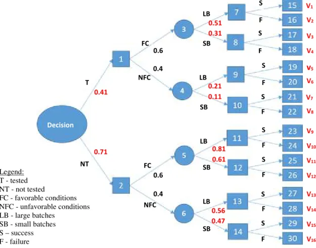
Decision tree it is a commonly used method in operational research, especially in data analysis and taking a decision choice depending on the conditions imposed and the objective being pursued.
The decision tree is a support tool in making a decision that translates into a graph with arcs and nodes. The arcs representing the activities to be done and the nodes are the events. Through this graph we can identify all available variants and their consequences.
This algorithm allowed the use of input data that are known with certainty but also some data that are known with probability. For the next demonstration I will use two elements found in any production enterprise, such as: the estimated profit share and the time to launch of a product.
Estimated profit share can be defined as the amount of money that is won by the enterprise after the end of the financial exercise, that is, the money that remains after the payment of all expenses.
The time to launch a product on the market - in this example, we will assume that it composed of: market sampled time to identify the optimal quantity released plus the time needed to prepare the release documentation in production.
The input data that are known for this demonstration are:
• The decision to choose for research or not to
the market belongs to the management of the enterprise and the time needed for the analysis and decision making is presented in table 2.1. There are two possibilities for each option. Favorable means that research activities are carried out according to the action plan and non-favorable it's that appear some delays occur.
Tab. 2.1. Research time (days)
Favorable Unfavorable
Testing 30 35
Without Testing 5 10
• The duration to launching in manufacturing is composed to all the activities necessary to start the manufacturing process (eg.: generating the documents necessary for the manufacturing process, the time to supply of
raw materials, the time for the
manufacturing planning, etc.). For this criterion there are two variants and the choice of one of the variants belongs to the management of the enterprise, namely: launching in large batches or small batches. Each variant can be launched in two ways. Successful launch means launching in as short a time as complete documentation. Launching with failure means launching late in production.
Tab. 2.2. The time to launch in manufacturing (days)
Success Failure
Large batch 15 18
Small batch 7 10
• Estimated profit share is the amount of money an enterprise expects to earn as a result of its business. These percentages are
estimated based on the amount
manufactured. The higher the amount products quantity, the fixed costs per unit of product are lower, which means that the estimated profit share will increase by maintaining the same price for the product. The same and for this criterion, there are two possibilities for each variant. Favorable is selling the products at the estimated price and unfavorably is representing the sale at a lower price, which means an estimated share of profit is lower.
Tab. 2.3. Estimated profit share
Favorable Unfavorable
Large batch 16 10
Small batch 9 5
The input data that are known with probability are largely influenced by the external menu of the organization:
• Favorable and unfavorable conditions - these can be identified by the competitive level on a certain segment of the market. For this example, the favorable conditions are
considered to be 60% and the unfavorable are 40%.
• Success or failure conditions - this criterion highlights the degree of absorption products by the market. Success conditions are approximately 70% (products are desired on the market) and failure conditions are 30%.
Fig. 2.1 The decision tree method
Step 1. Determine the economic consequences of each branch. As a mentioned above, the two consequences are: the profit estimated and the time to launch
= ∗ [euro] (1) where:
- Cje = estimated profit share - P = estimated profit
- Qi = the quantity launched
DTL = DSi + DSFj [zile] (2) where:
- DTL = the time to launch in manufacturing - DSi = the research time
- DSFj = the time required for launch in manufacturing
Step 2. Determine the usefulness of each criterion. Due to the fact that the two criteria have different units of measurement, these cannot be used in this algorithm. Bringing them to a common unit of measurement requires the application of the utilities method. The usefulness of a criterion can have a value in the range of [0-1], 0 means unnecessary and 1 means the maximum degree of utility
=
(3)
where:
- uij - the usefulness of the criterion ‘i’ for the variant ‘j’
- aij - consequence of criterion "i" for variant "j"
V3
V4
v5
V6
V7
V9
V10
V11
V12
V13
V14
V15
0,41
0,71
V16
T
NT
NFC NFC
FC
FC
LB
LB
LB
LB SB
SB
SB
SB
S
S
S
S
S
S
S
S
F F F F F F F F
V1
V2
V8
Decision
Legend: T - tested NT - not tested
FC - favorable conditions NFC - unfavorable conditions LB - large batches
SB - small batches S – success F - failure
0.41
0.71
0.6
0.6
0.4 0.4
0.51 0.31
0.21 0.11
0.81 0.61
- a0 – the unfavorable consequence of the criterion ‘i’
- a1 – the favorable consequence of the criterion ‘i’
Step 3. Determination of the values obtained at the end of each economic branch. After obtaining the utility coefficients for both criteria and all variants, these will multiply with the coefficient of importance (kj).
= ∗ ( + ) (4)
where:
- vi – the expected value for each variation „i”;
- kj= the coefficient of importance for each criterion;
- ui1 – the usefulness of the criterion 1 for the variant „i”;
- ui2 – the usefulness of the criterion 2 for the variant „i”;;
Step 4. The expected mean values in the points 3, 4, 5 and 6. At this stage, all the mean values expected in the points above will be calculated according to the following formula. The values at the end of each economic branch will be multiplied by the probability coefficient corresponding to the respective variants.
= ∗ + ∗
Nod 3 (5)
= ∗ + ∗
Step 5. Determine the expected mean values in the Decision points:
= ∗ + ∗
Decision (6)
= ∗ + ∗
Once it has reached the top of the decision tree, the economic branch that brings the greatest benefits can be identified. According to the
defined input values, the company's
management will choose: not to test the market, to have favorable conditions and to launch large batches in manufacturing.
3. DIMENSION TIME OF FABRICATION AND THE TRANSMISSION MODE FOR
THE MANUFACTURING BATCHES
BETWEEN OPERATIONS
3.1. The manufacturing cycle
The manufacturing cycle is a sequence of activities whereby the raw materials and materials pass in an organized way on the technological flow to be transformed into semi or finished products.
The length of the fabrication cycle is a very important factor in the manufacturing process and consists of the time between the start of the first operation and the finish of the last operation from the technological process. The length of the fabrication cycle is influenced by several characteristics: the size of the items to be manufactured, the size of the batches, the type of means transport used in the production process, the level utilization of the production capacities and the way of using to the current assets company’s. The shorter of the production cycle, the lower the amount of circulating assets invested in unfinished production.
.
The duration of manufacturing cycle
Operational time
The duration of interruptions
Base time
The time to preparing the
operation
the time for natural processes
Breaks in work hours
Breaks in out of work hours
Scheduled interruptions
Interruptions generated by the manufacturing
capacity
Breaks due the batch’s
Fig. 3.1 Types of time from the structure of manufacturing cycle The size of the fabrication cycle can be
directly influences the productive, economic and financial activity of industrial enterprises and makes their profitability conditional.
The structure of the fabrication cycle can be defined as the totality of the component elements used in the manufacturing process. It is necessary to know all the elements for the determination of the total duration and for the identification of the technical and organizational measures that can be taken in order to reduce the duration of the manufacturing cycle
The structure of the manufacturing cycle may be including two major categories of time, namely: operational times and interruptions, as shown in Figure 3.1
Operational Times - this category includes times for different types of activities encountered in the manufacturing process. • base time - is the effective time to the
intervention on raw materials. The
transformation can be: the form, the structure, the size, the properties, etc.
• the time required for preparing and finishing
the operation - is a very complex time, consisting of: the time of studying the technical documentation, the time to fixing and removing of the semi-finished; time to prepare the tools and devices, time to bring the machine to the required operating
parameters, the time to check the
dimensions, the time to remove the waste from the active area of the machine, etc.
• the time required for natural processing -
is the mandatory time that cannot be removed after performing some operations, for example: drying time after the painting operation or the cooling time after the heat treatment, etc.;
= ∑ + + (7)
where:
- to= operational time;
- tbk – base time the operation k;
- tnpk – natural processes time the operation k; - tpk – preparation time for operation k; - k – operation number of the manufacturing
cycle;
- m – total number of operations in the manufacturing cycle.
The interruptions periods in the manufacturing process - are divided in two major categories, namely: breaks in work hours and in out of work hours. This division is due to the length of the manufacturing cycle which is divided into time units (hours, days, weeks, months and years).
The interruptions in out of working time can be caused by two factors:
• the first factor - is generated due to legal free days until the manufacturing process is resumed (eg Saturday, Sunday, legal holiday). These interruptions occur when the manufacturing cycle of the product lasts for more than a week.
• the second factor - is generated due to work on shifts, the occurrence of interruptions until the manufacturing process resumes (eg: shift change).
= ∑( + + + ) (8)
where:
- tintr= the duration interruption - tsi = scheduled interruptions - tbb = breaks due the batch’s
- tbmc = interruptions generated by the manufacturing capacity
- tvci = verification and control interruptions
The technical and organizational breaks - these occur during in the schedule time and consist into several types, the most important being represented in Figure 3.5, namely:
• scheduled interruptions - this category will be including: lunch break, rest break, physiological needs, etc., which are mandatory by law
• interruptions generated by the manufacturing capacity of each working place - is the time when the batch is waiting for the release of the working place that are occupied with other batches / items. These interruptions are characteristics by the homogeneous group of machines;
• verification and control interruptions - is the time when the items are waiting in the area of temporary safety deposit to created inside the fabrication unit for quality control;
3.2. Transmission methods of the
manufacturing batches between operations
In the literature, there are several methods published to send a batch of items between operations. Depending on the mode of transmission chosen will be generated a number of advantages and disadvantages. Choosing the best method belongs to the management decision of the enterprise that will choose between the requirements of the product's technology, the available resources, the goals of the enterprise or other conditions.
The three modes of batches transmission between operations are successive, parallel and mixed method.
The manufacturing batch can be defined as a finite set of similar items that follows the same sequence of operations with the same preparation time and the shift from one machine to another will be done at the same time for the whole batch.
For each of the above-mentioned methods, there are two variants of solving, one analytical and one graphic. It should be noted that either of the two methods we apply should achieve the same result.
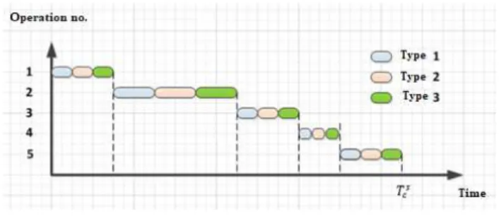
Determined time transmission of
manufacturing batches by applying the
successive method, in the analytical and graphic variant.
The analytical variant
= ∗ ∑ i=1,k (9)
where:
- n = number of items from o batch; - k = the number of operation;
- ti = the time for each operation „i”.
The graphic variant.
Fig. 3.2 The successive method
Advantages of this planning type: • simple resource planning
• efficient use of resources • reduced costs
Disadvantages of this planning type
• the duration of manufacturing cycle is high
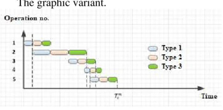
Determined time transmission of
manufacturing batches by applying the parallel method, in the analytical and graphic variant.
The analytical variant
= ∑ + ( − 1) i=1,k (10)
where:
- n = number of items from o batch; - k = the number of operation; - ti = the time for each operation „i”.
The graphic variant.
Fig. 3.3 The parallel method
Advantages of this planning type:
• the duration of manufacturing cycle is short • simple resource planning
Determined time transmission of manufacturing batches by applying the mixed method, in the analytical and graphic variant.
The analytical variant
= ∑ + ( − 1) + ∑ , (11)
i=1,k
∑, = ( − )( − 1) ti>tj (12)
where:
- n = number of items from o batch; - k = the number of operation; - ti = the time for each operation „i”.
The graphic variant.
Fig. 3.4 The mixed method
Advantages of this planning type:
• the duration of manufacturing cycle is short • efficient use of resources
• reduced cost
Disadvantages of this planning type • complex resource planning
All the methods presented are good but these must be applied correctly depending on the conditions and goals company's
4. CONCLUSION
In any decision taken within an enterprise there are two essential elements that are in a
strong correlation. Changing an item
automatically affects the other who may or may not improve the business.
There is no decision in an enterprise that does not include the "time" element, because it is considered as the basic unit for measuring the duration of the activities undertaken.
Any activity undertaken by an enterprise is carried out in order to generate the profit for a certain period. The assumed decisions should be substantiated by modern methods and tools for processing the data on which selection is to be made.
The decision tree is one of the most effective ways to make a decision. This method provides the possibility to define several types of variables used as input into a system, some of which can be known with certainty and others with probability.
The second solution offered is a method for
sizing the manufacturing cycle. Any
management of an enterprise wishes to know
before starting to work as long the
manufacturing process for the desired product lasts. The solution presented can be personalized according to the user's needs by removing or adding additional time depending on the field of activity and the manufacturing process.
The latter solution highlights how the manufacturing batches can be transmitted between operations in relative to the time axis. All of three methods presented are effective, but choosing the most appropriate option is based on the conditions in the production unit and management objectives.
5. REFERENCES
[1] Cicalese, F; Laber, E.; Saettler, A. Decision Trees for Function Evaluation: Simultaneous Optimization of Worst and Expected Cost, Algorithmica, Vol: 79, Issue: 3, Pages: 763-796; 2017.
[2] Pugna, A; Mocan, M; Feniser, C Using Six Sigma Methodology to Improve Complex
Processes Performance, International
conference on production research - regional conference africa, europe and the middle east Pages: 18-23, 2016
[3] Filip D., Lungu F., The management of small and unique production series, LAP LAMBERT Academic Publishing, ISBN-13:973-3-659-31753-8, Germany, 2013. [4] Florica, B., Managementul producției,
Publisher ALL, ISBN: 9735491554,
[5] Abrudan, I., Cândea, D. (coord.), Programarea producției de unicate, Manual de Inginerie Economică - Ingineria si Managementul Sistemelor de Producție., Editura Dacia, ISBN: 973-35-1588-4, Cluj-Napoca, 2002.
[6] V. Firescu, R. Vlad, N. Toderici, “The Application of the Lean Management Principles and Methods - Opportunities and
Hedges from the Romanian Employees,”
Proceedings of the 1st Management
Conference: Twenty Years After - How Management Theory Works, Cluj-Napoca, 2010, pp. 73-89.
[7] https://www.britannica.com/technology/ production-management
Aplicarea unor metodelor matematice pentru optimizarea procesului de lansare în fabricație
Această lucrare scoate în evidență principalele elemente ale procesului decizional cum ar fi timpul și profitul, acestea fiind într-o strânsă legătură. Orice întreprindere producătoare își dorește să obțină
cele mai eficiente decizii care să genereze rezultatele scontate. Pentru îmbunătățirea activității de luare a deciziei de lansare a unui produs nou in fabricație este prezentată metoda Arborelui decizional iar pentru gestionarea eficientă a ciclului de fabricație sunt prezentate cele trei metode: succesivă, paralelăși mixtă.